
Abstract
The decomposition of the overall effect of a treatment into direct and indirect effects is here investigated with reference to a recursive system of binary random variables. We show how, for the single mediator context, the marginal effect measured on the log odds scale can be written as the sum of the indirect and direct effects plus a residual term that vanishes under some specific conditions. We then extend our definitions to situations involving multiple mediators and address research questions concerning the decomposition of the total effect when some mediators on the pathway from the treatment to the outcome are marginalized over. Connections to the counterfactual definitions of the effects are also made. Data coming from an encouragement design on students’ attitude to visit museums in Florence, Italy, are reanalyzed. The estimates of the defined quantities are reported together with their standard errors to compute p values and form confidence intervals.
Keywords
Introduction
The decomposition of the total effect of a treatment X on an outcome variable Y into direct and indirect effects is a central topic in empirical research. In linear models, the relationship between total, direct, and indirect effects is well understood (Alwin and Hauser 1975; Bollen 1987; Baron and Kenny 1986; Cochran 1938) and a simple decomposition is available. Such a decomposition is based on the linearity of the marginal model for Y against X, where the coefficient of X is equal to the sum of the direct effect and the indirect effects. Outside the linear case, this simplicity is lost, as in the marginal model of Y against X only, either the effect of X on Y is a complex function of the original parameters or the error term does not possess nice properties or both.
We here consider situations where the outcome Y is a binary random variable. Contributions have addressed the case of one continuous mediator (see, e.g., Breen, Karlson, and Holm 2013, 2018; Karlson, Holm, and Breen 2012; MacKinnon et al. 2007). Recent results concern the exact parametric form of the marginal effect of X on Y on the log odds ratio scale when the mediator is also binary (Stanghellini and Doretti 2019). In this setting, when X is continuous the marginal model of Y against X is nonlinear unless some conditional independence assumptions hold, and a rather complex formula links the marginal and conditional effect of X on Y. Similarly, for a discrete X, the parameters of the conditional model combine in a nonlinear fashion to form the marginal effect. For analogous results on the log relative risk scale, see Lupparelli (2019).
Starting from the results in Stanghellini and Doretti (2019), we here elaborate a novel proposal for the direct and indirect effect definitions on the log odds scale for a treatment variable X either continuous or discrete. The postulated system can be represented by a directed acyclic graph (DAG); see Lauritzen (1996, chap. 2), to which we refer for definitions, see also Elwert (2013) for an account in the sociological context. Our proposal is based on zeroing the path-specific regression coefficients. Graphically, this corresponds to deleting one arrow in the associated DAG and thereby represents the analogue of the path analysis method.
We initially focus on a single-mediator context and show that the marginal effect can be written as the sum of the indirect and direct effects plus a residual term that vanishes under some specific conditions. The proposed parametric relationship allows, for the specific setting under investigation, to solve the debate on which method should be used to disentangle the total effect, that is, the product method or the difference method (Breen et al. 2018). It also avoids fitting two nested models, thereby sidestepping the issue of unequal variance (Winship and Mare 1983). We then extend our derivations to the case of multiple binary mediators, also modeled as a recursive system of univariate logistic regressions. In this context, additional path-specific effects can be defined and different research questions addressed. Although the paper draws from the derivation in Stanghellini and Doretti (2019), some novel results are also presented. With reference to a single mediator, a general formulation of functional form linking the log odds of the mediator and of the outcome to the covariates is considered. This is then extended to the multiple mediator context, for which a strategy for deriving the direct and indirect effects when marginalizing over an intermediate or outer mediator is also illustrated.
Our approach is developed in a purely associational context that, in general, holds no interpretation for causal inference. However, if the recursive system of equation is structural (Pearl 2009, chap. 7) and no unmeasured confounders exist, the total effect and some of its components can be endowed with a causal interpretation. Notice that a decomposition of the total effect based on counterfactual entities has been given by Pearl (2001, 2012) and extended to the odds ratio scale by VanderWeele and Vansteelandt (2010). This parallelism is also addressed in this article.
In the second section, we offer the general theory for the case of a single mediator. A case study concerning a randomized encouragement experiment on cultural consumption performed in Florence (Italy) is also presented as a guiding example. Results of a simulation study investigating maximum likelihood (ML) estimation of the effects and other related measures is also reported in the third section, while the extension to the multiple mediator setting is contained in the fourth section. In the fifth section, we address other complex issues concerning path-specific effects, whereas links with counterfactual definitions are explored in the sixth section. Finally, in the seventh section, we draw some conclusions.
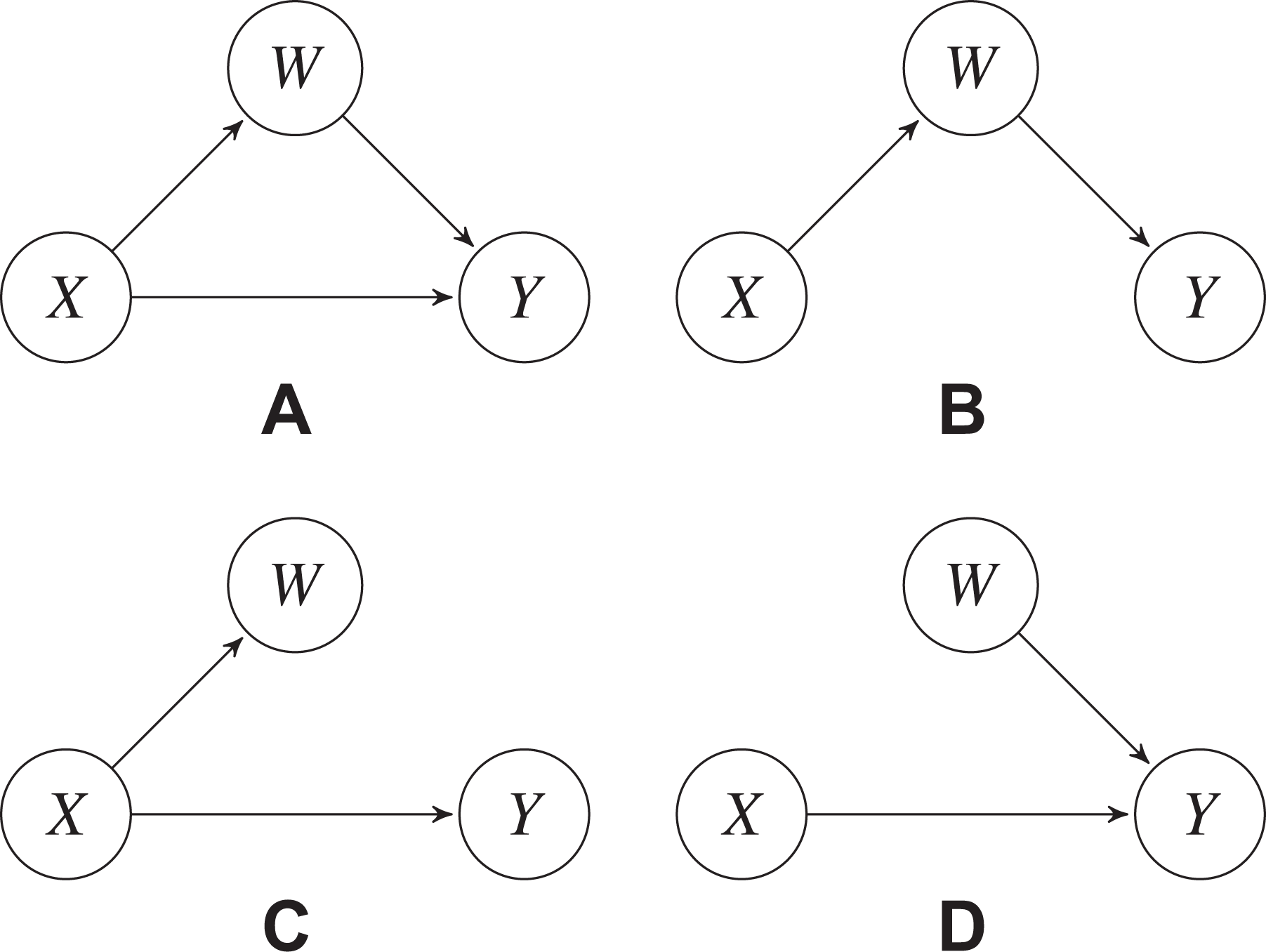
Data generating process when (A) no conditional independences hold, (B)
Effect Decomposition With a Single Mediator
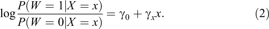
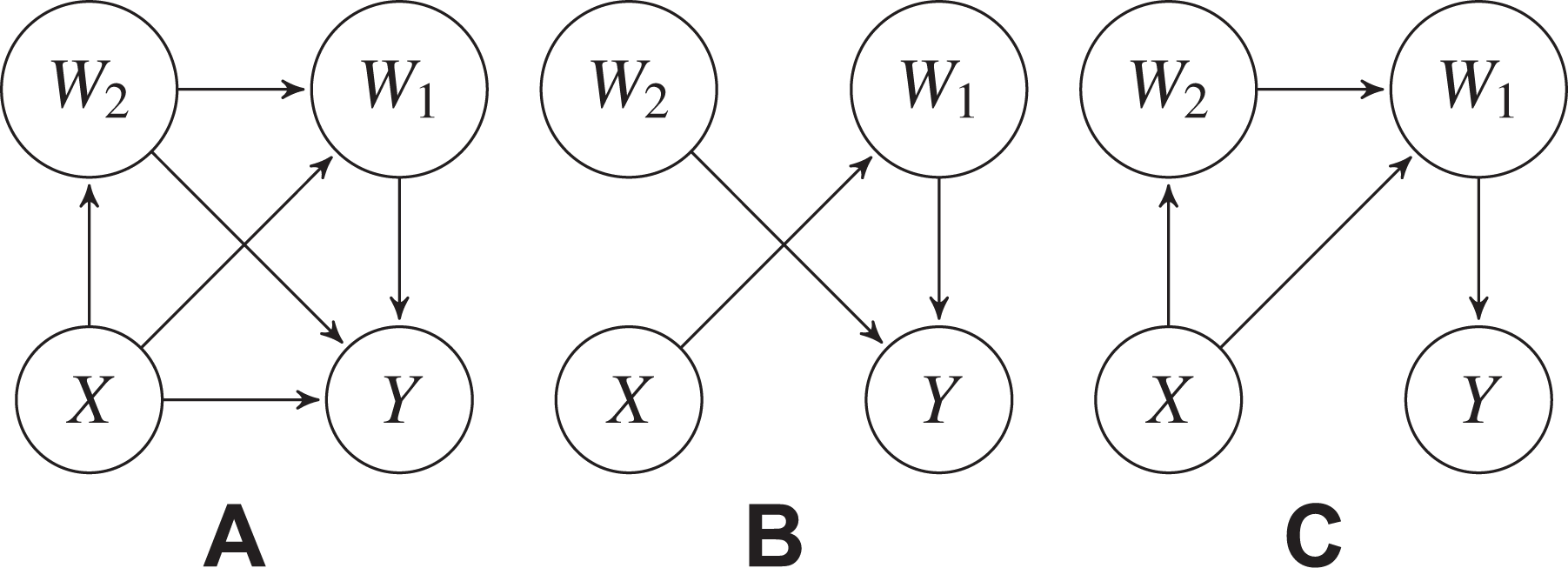
We first focus on a very simple model for a binary outcome Y, a binary mediator W, and a treatment X, that can be either discrete or continuous (see Figure 1A for the corresponding DAG). Our aim is to decompose the total effect of X on Y on the log odds scale. Our postulated models are a logistic regression for Y given X and W and for W given X, that is,

and
Notice that we allow for the interaction between X and W in the outcome equation. In order to make the paper self-contained, the derivations in Stanghellini and Doretti (2019) to evaluate the total effect as a function of the parameters of models (1) and (2) are here reproduced, prior the introduction of its decomposition into direct, indirect, and residual effects.
As a guiding example through this section, we consider an experiment aiming at identifying the best incentives to offer high school students in Florence to enhance cultural interest and increase art museum attendance. Three treatment levels are considered: A flyer given to the students with the main information about the Palazzo Vecchio museum constitutes the first level; a flyer and a presentation of the museum from an expert constitute the second level; a flyer, the presentation, and a reward in the form of extra-credit points for their final school grade constitute the third level. All students receive a free entry ticket to Palazzo Vecchio. The aim of the experiment is not only to assess the total effect of the treatment (X) on students museum’s attendance (Y) but also to understand to what extent this effect could be stimulated by student’s visit to Palazzo Vecchio (W); see Forastiere et al. (2019); Lattarulo, Mariani, and Razzolini (2017).
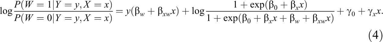
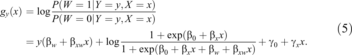
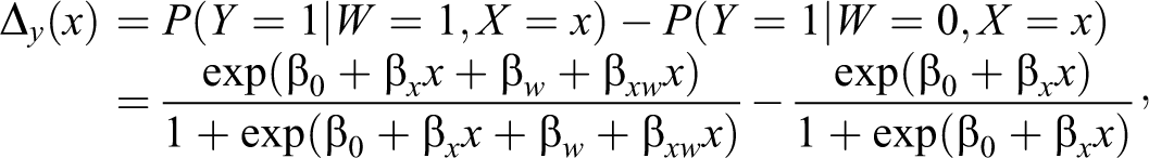
The interest is in the marginal model of Y against X, as a function of the parameters in equations (1) and (2). From first principles of probabilities, it follows that:

The second term of the righthand side (RHS) of the above equality is given from model (1), while the parametric expression of the first term is not immediately derived from models (1) and (2), as it involves the probability of W after conditioning on X and Y (not after conditioning on X only). However, by repeated use of the previous relationship, we have:

Using equations (1) and (2), after some simplifications, we find:
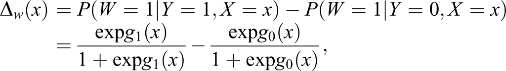
In what follows, we denote with
Since

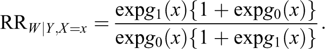
Denoting with

the relative risk of W for varying Y in the distribution of
Analogously, letting
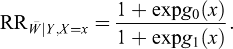
It then follows that equation (6) can be rewritten as

or, alternatively, as

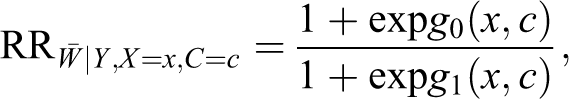
Notice that conditioning on a set of covariates
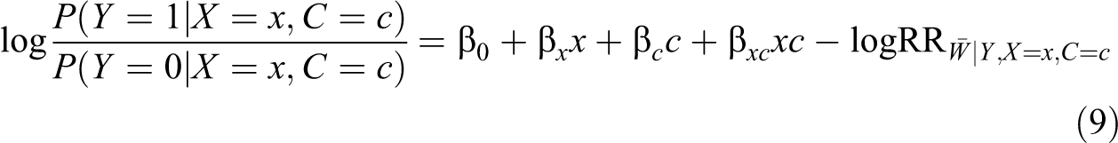
with
and
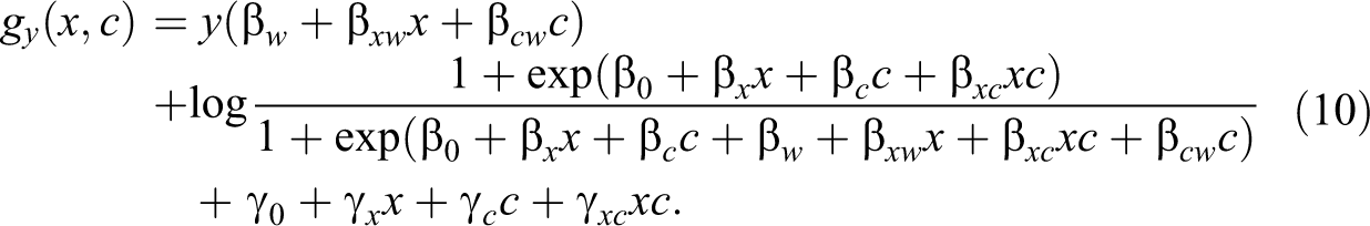
See Online Appendix A (Supplementary material for this article is available online) for a general formulation that includes more covariates and possibly nonlinear link functions.
With reference to the cultural consumption data, 15 classes for a total of 294 students, all aged between 15 and 18, from three different schools, were randomly assigned at baseline (March/April 2014) to the three treatment levels (X). At the second occasion, after two months, researchers collected the entry tickets to record student visits (W). Finally, after six months, they collected the concluding questionnaire with general information on visits to other museums (Y). A questionnaire with information on background characteristics of the students and their families was also administered. Among all the covariates, only one appears to be relevant in the model for the outcome, that is, the binary variable C taking value 1 for students considering themselves mainly interested in mathematics/science and 0 if they are mainly interested in humanities. At follow-up, 28 students were absent, so the final sample included 266 students. Data are reported in Table 1 and are publicly available at https://www-tandfonline-com-s.web.bisu.edu.cn/doi/abs/10.1080/07350015.2019.1647843 as supplementary material of Forastiere et al. (2019).
Contingency Tables for (
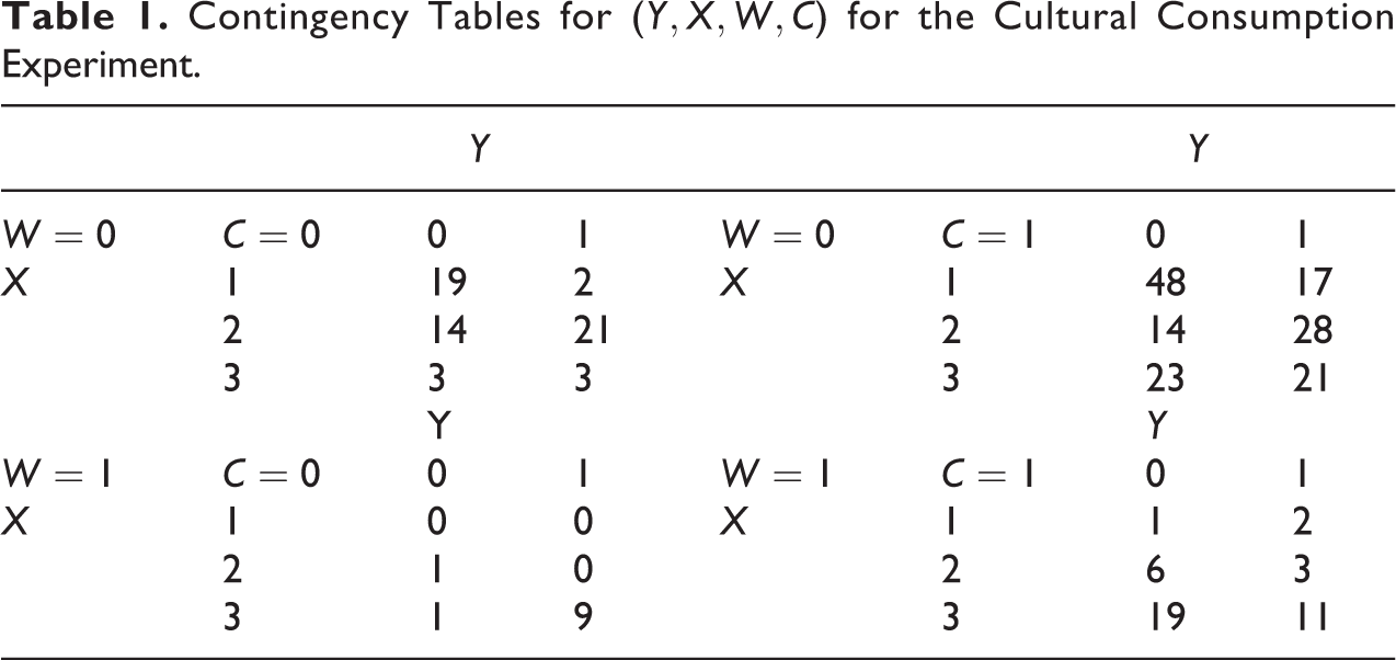
Table 2 contains the output of the ML estimation of the logistic regression models for the outcome and for the mediator. We use the subscript
Maximum Likelihood Estimates of the Two Logistic Models for Y and W for the Cultural Consumption Experiment.

Ignoring for now the sampling errors, we see that the
We now present a definition for the total, direct, and indirect effects in the situation with no covariates. When covariates C are present, the parametric formula of
Total effect: Let
Indirect effect: Let
Direct effect: Let
Residual effect: Let

Notice that this residual term is always null in linear models. In this context, the total effect can be decomposed into the sum of the direct and indirect effect. Provided that these two are positive, it is therefore meaningful to look at the ratio between the indirect effect and the total effect, as it gives an indication of the proportion of total effect due to the mediator W (i.e., the proportion mediated). When a residual effect is present, the ratio between the indirect and total effect can still provide information on the weight of the indirect effect on the total effect, though with a less clear interpretation (see Continuous Case and Discrete Case subsections).
In what follows, we study in detail the decomposition of the total effect for the simple case without covariates, where X can be either continuous or discrete. Addition of covariates can be done in a straightforward manner.
Continuous Case
We first look at the case of X continuous and differentiable. Let
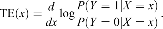
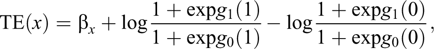
It is possible to show that
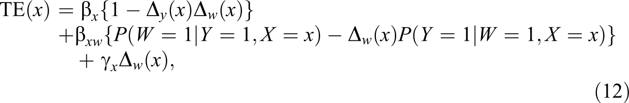
where
and
with
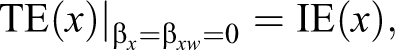
Indirect effect: Following the definition, we evaluate the total effect assuming

where
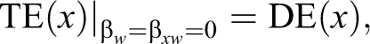
Direct effect: Following the definition, we evaluate the direct effect after assuming

Notice that equation (14) follows as
Residual effect: Finally, the residual effect is given by difference as follows
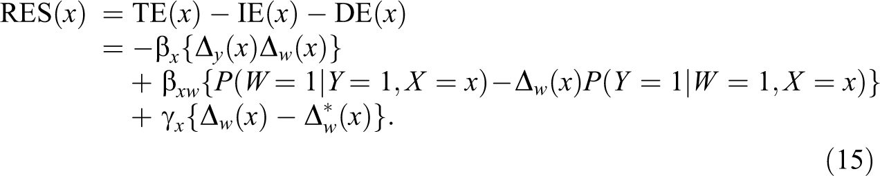
It is therefore apparent that the effect above vanishes whenever
Some cases of interest: Reformulating the total effect by definition as in equation (11), we study in detail the decomposition of the total effect into indirect (equation [13]), direct (equation [14]), and residual (equation [15]) effects for some cases of interest.
Case (i) When the recursive logistic models can be depicted as in Figure 1B, that is,
and both
Case (ii) When the recursive logistic models can be depicted as in Figure 1C, that is,
and both
Case (iii) A noticeable situation arises after imposing

where

Notice that this assumption does not itself reflect into any conditional independence. If we further assume

where

It is possible to see that under this condition,
Case (iv) When the recursive logistic models can be depicted as in Figure 1D, that is,

where

In this case, there is an effect modification due to conditioning of an additional variable, in line with well-known results on noncollapsibility of parameters of logistic regression models (see Xie et al. 2008). In addition, we notice that even in this simple case, the linearity of X in the marginal model is lost. Furthermore, if
Discrete Case
Without loss of generality, we here assume that X is binary. The total effect of X on Y can be derived by taking the first difference of, equivalently, equations (7) or (8). We here opt for differentiating equation (7). Then,

which explicitly becomes
with
Indirect effect: Following the definition above, we evaluate the total effect assuming

where
Direct effect: Following the definition of the direct effect, we evaluate the direct effect after assuming in the total effect

Residual effect: By definition, the remaining effect is evaluated by difference, such as
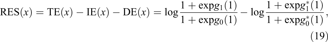
with
Some cases of interest: Following the definition, we reformulate the total effect of a binary X on a binary Y as in equation (11) and we study in detail the decomposition of the total effect into the indirect (equation [17]), direct (equation [18]), and residual (equation [19]) effects for some cases of interest.
Case (i) When the recursive logistic models can be depicted as in Figure 1B, that is,

and both
Case (ii) When the recursive logistic models can be depicted as in Figure 1C, that is,

as all other terms are zero.
Case (iii) After imposing

in which
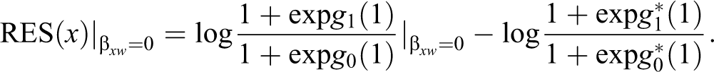
Notice that
Case (iv) When the recursive logistic models can be depicted as in Figure 1D, that is,

where

After some algebra, it is possible to show that this condition is sufficient to avoid effect reversal as proved by Cox and Wermuth (2003) in a more general context.
With reference to the cultural consumption data, in Table 3, the decomposition of the total effect of moving from level 1 to the other levels of X is reported. Notice that this decomposition is based on the estimated parameters of Table 2 and does not require to estimate the marginal model of Y against X and C only, thereby avoiding the issue of comparing parameters coming from two logistic models with unequal variance. The 95 percent confidence intervals and p-values are calculated using the approximated standard errors evaluated via the delta method (Oehlert 1992).
Estimates (Est.), Standard Errors (SEs), 95 Percent Confidence Intervals (CIs), and p Values of the Effects for the Cultural Consumption Experiment.

In the upper part of Table 3, the decomposition for the
In summary, the direct and total effects of moving from level 1 to level 2 of X are positive and statistically significant in all groups of students, while the indirect effect, also positive, is significant only for students mainly interested in humanities. When moving from level 1 to level 3 of X, all effects are positive and significant. We believe that this is an important message on how to design incentives to increase museums attendance of high school students which cannot be easily derived by simply looking at the estimated coefficients in Table 2.
Our results are aligned with the ones in the original studies. Lattarulo et al. (2017) estimated an average causal effect based on the mean difference and the difference in difference methods, marginally with respect to W. Instead, in the study of Forastiere et al. (2019), the authors performed a decomposition of the total effect based on counterfactual entities using the principal stratification method.
Effect decomposition on the probability scale
So far, we have considered effect decompositions operating on the logistic scale. However, sociologists and econometricians are quite often concerned with effects on the probability scale (also called partial effects; see Wooldridge 2010, chap. 15), for which effect decompositions in specific contexts, typically on the additive scale, have also been proposed (Breen et al. 2013; Karlson et al. 2012). We here denote with

For the continuous

where
On the other hand, for X binary or discrete, the total effect on the probability scale can be defined by simply taking the difference across levels of X of the marginal probability. For the binary X, this becomes:

In analogy with the approach of the second section, the direct probability effect

With particular reference to the continuous case, this amounts to:

where
with the average direct probability effect (ADPE) and the average indirect probability effect (AIPE) defined analogously. However, these average effects should be taken with caution when there is a strong variation across values of x.
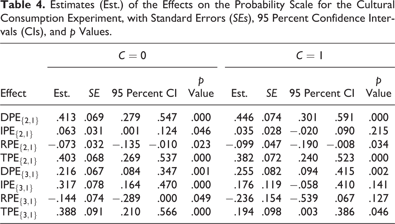
For the cultural consumption data, the effects on the probability scale are summarized in Table 4, which has the same structure of Table 3. As expected, results are in line with the ones on the log odds scale. Notice that averaging the effects may be not appropriate in applications with a strong variation across levels of x, as in this case, especially with reference to the indirect effects.
Estimates (Est.) of the Effects on the Probability Scale for the Cultural Consumption Experiment, with Standard Errors (SEs), 95 Percent Confidence Intervals (CIs), and p Values.
Simulation Study
In this section, we present results of a simulation study to investigate how well the relative amount of indirect effect is recovered, also in relation with already existing methods. In particular, Karlson et al. (2012) and Breen et al. (2013) derive a decomposition of the total effect that can be applied to the case of a continuous mediator W, when the response model for Y can either be a logistic or a probit one with no interaction terms. In this context, the total effect, as measured by the marginal coefficient of X on Y, is the sum of the direct and indirect effects as in linear models. When all effects are positive, it is therefore meaningful to compute the proportion mediated as the ratio between the indirect and total effect (see Equation [21] in Breen et al. 2013). The authors present a method to sidestep the well-known issue of unequal variances, known as the Karlson Holm and Breen (KHB) method. They also propose to adapt it to the binary mediator case, by postulating a linear probability model for W.
We here postulate a logistic model for W and analyze, through simulations, the behavior in finite samples of the KHB method and of the proposed method. For X binary, we compare the KHB method with the ratio between the estimates of the effects IE(x) and TE(x) in the second section, obtained by plugging-in the ML estimates of the parameters in the corresponding expression. For X continuous, we notice that the KHB measure should be interpreted as the proportion mediated on the probability scale in the same fashion as discussed in Effect Decomposition on the Probability Scale subsection. For this reason, we proceed as follows. Given a sample of n units, an estimate of the corresponding effect is formed by averaging across units the corresponding entities. As an instance, the estimated ATPE is so formed:
where
We consider a basic setting with no covariates, where the outcome Y and the mediator W are generated according to Equations (1) and (2) respectively. Though our method can accommodate for the treatment–mediator interaction
We define three sample sizes, that is,
Table 5 summarizes the simulation results. Notice that for X binary, the dependence of
True Value and Simulation Average, Variance, and Root Mean Squared Error (RMSE) for the KHB Method and the Proposed Method (RSD).
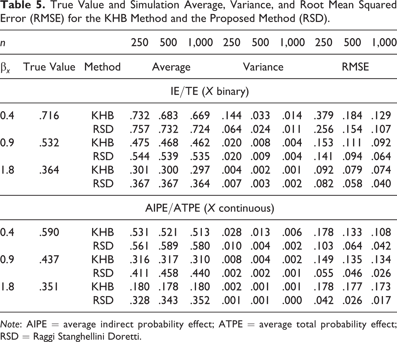
Note: AIPE = average indirect probability effect; ATPE = average total probability effect; RSD = Raggi Stanghellini Doretti.
Extension to Multiple Binary Mediators
The proposed definitions of direct, indirect, and residual effects, together with their parametric formulations, extend nicely to the situation where multiple binary mediators are present. Suppose there are k mediators and that a full ordering among the variables
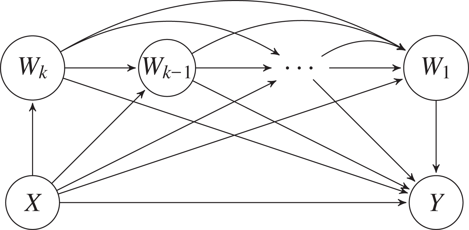
Directed acyclic graph with k mediators.
In analogy with equation (7), the logistic model for Y given X, obtained after marginalization upon the k mediators, is
where
In Online Appendix C (Supplementary material for this article is available online), the relevant expressions are given.
In line with what done for the simple case, we here offer a generalization of the definitions for the total, direct, indirect, and residual effects under the situation of k mediators.
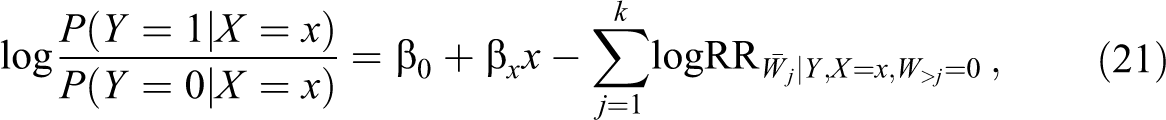
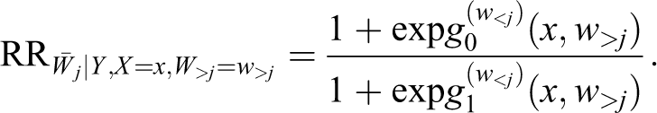
Total effect: Let
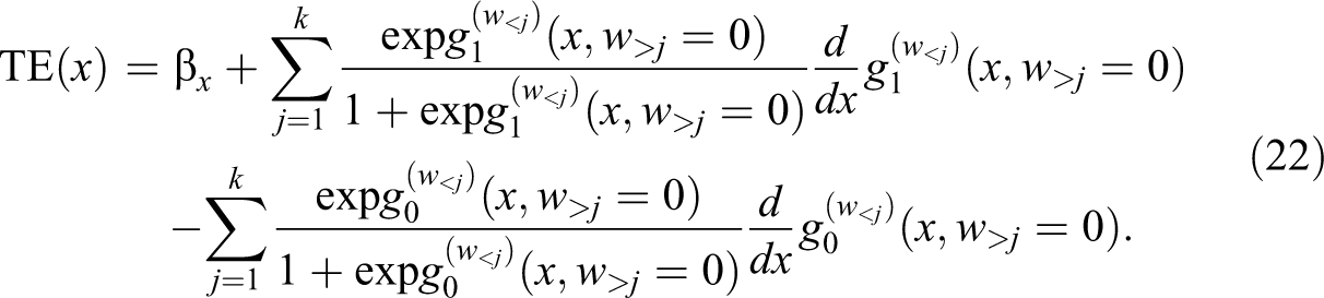
For X discrete, the total effect is defined as the difference between equation (21) evaluated at two different levels of X. Without loss of generality, we here assume X binary and take the difference for
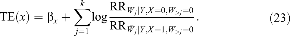
Equation (23) can also be written as follows

Direct effect: Let

Global indirect effect: The global indirect effect

Residual effect: Let

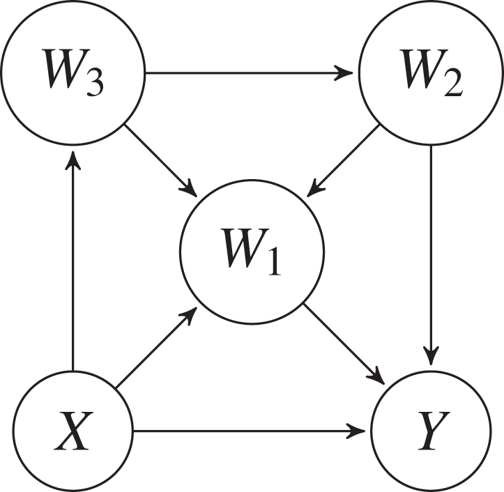
From previous derivations, nonzero residual effects are induced by graphs having more than one arrow pointing to Y. Therefore, we can state that the residual effect is zero whenever one of the two following graphical conditions holds: (i) there is no direct path from X to Y or (ii) there is the direct path from X to Y and no other arrow is pointing to Y. As an instance, the model corresponding to the DAG in Figure 3A has a nonzero
Directed acyclic graphs with
In a setting with multiple mediators, one is also interested in a path-specific indirect effect, that is, the effect that is due to some mediators only, and is null whenever one arrow along the pathway is deleted. Notice that, in this setting, also other research questions are of interest, such as the path-specific indirect effects when some mediators are marginalized over. They are addressed in the fifth section.
Path-specific indirect effect: Let A be one of the
In this way, each path-specific indirect effect contains only the parameters pertaining to the path (including the intercepts). It then follows that the indirect effect
Notice that each of the conditions above implies deleting one arrow in the DAG corresponding to the model of interest.
As an instance, let
where
Notice that the definition of path-specific indirect effects allows only for direction preserving paths, that is, paths with all arrows pointing to the same direction. As a matter of fact, only ordered subsets of W are allowed to form A. This choice is justified by the fact that these are the only subsets with a nonzero path-specific indirect effect. To clarify the issue, see the graph in Figure 4. The path
Directed acyclic graph with W
1 acting as a collider node in the path
It is also important to notice that, in parallel to the single-mediator case,
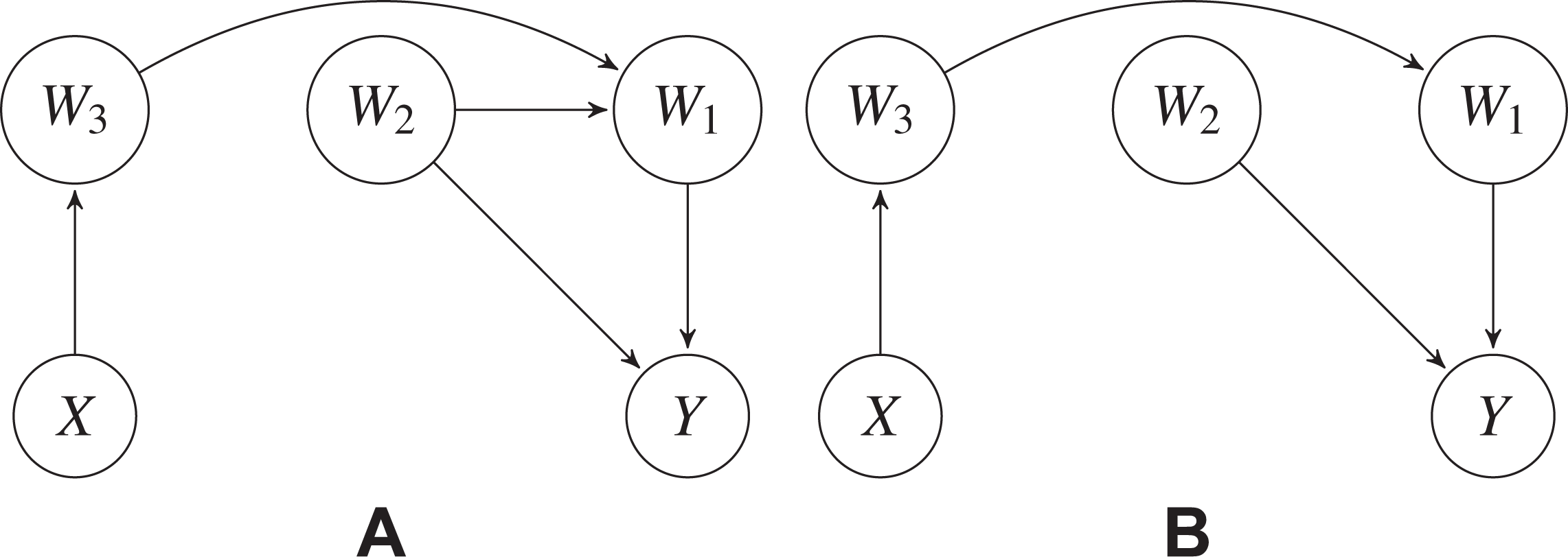
Notice that the sum of all the path-specific indirect effects in general is not equal to the global indirect effect. This is true even when there is just one path from X to Y. This is due to the different ways to deal with the effects induced in noncollapsible subgraphs. These are subgraphs involving three random variables,
As an example, consider the models with DAG as in Figure 5A and B. In both DAGs, there is just one indirect path leading from X to Y, that is,
Directed acyclic graph with
Other Path-specific Indirect Effects of Interest
Suppose now that the research question involves path-specific effects in the model obtained after marginalization over some mediators while others are kept in the model. First of all, the parameters of the marginal model of interest should be obtained and then the path-specific indirect effects can be evaluated. Two different situations may arise. The first one involves marginalization over an inner mediator, and therefore equation (21) can be used in a straightforward manner. The second one involves marginalization over one intermediate/outer node and more technicalities are necessary. We here present an instance of both situations.
Suppose that the research question involves investigation of the path-specific indirect effects in the model obtained after marginalization over W
1 of a model corresponding to the DAG in Figure 6A. In Figure 6B, the DAG corresponding to the marginal model of interest is presented, with the red arrows corresponding to parameters that change due to the marginalization over W
1. The expressions for these parameters is reported in Online Appendix D (Supplementary material for this article is available online). The only nonzero path-specific indirect effects are for
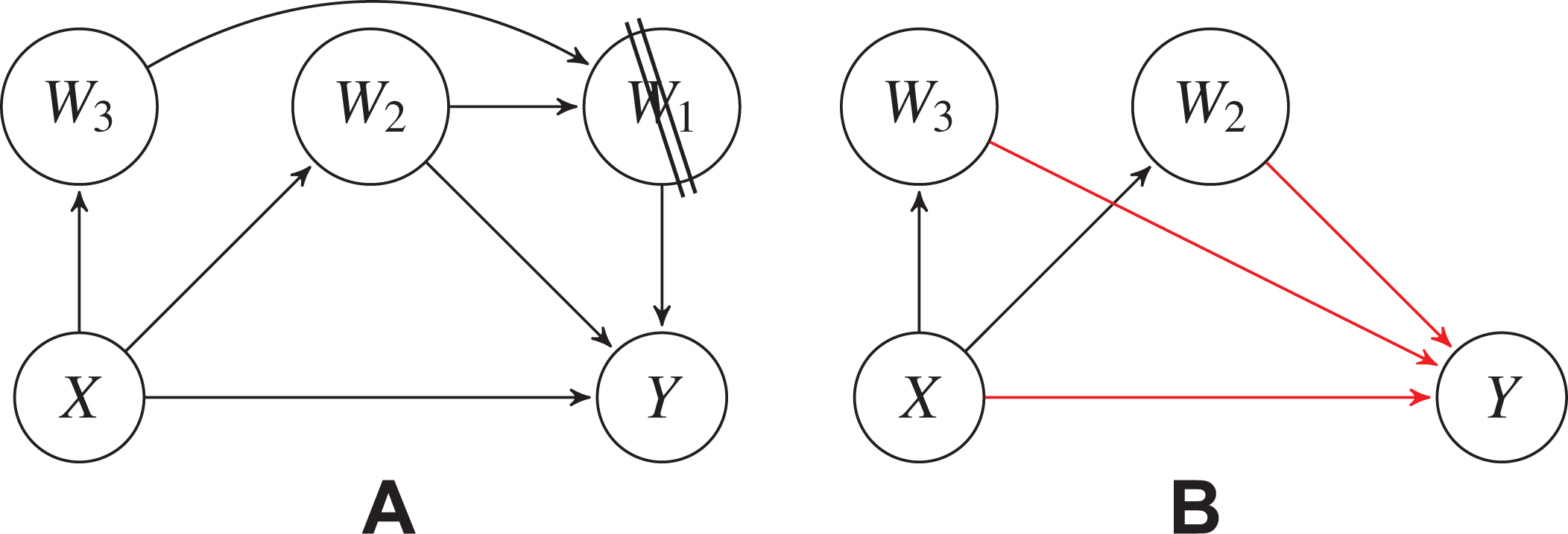
(A) Marginalization over the inner mediator W 1 and (B) quantifying the parameters (in red the parameters that change).
Quantification of effects in models obtained after marginalization over intermediate or outer nodes involves repeated use of the derivations here presented. We here detail the steps to be followed for the case with
Suppose that we wish to evaluate the indirect effect in the model with W 1 as unique mediator, that is, the model obtained after marginalization over W 2 (see Figure 7). This implies deriving the parametric formulation of
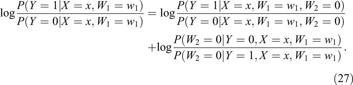
in which the second term of the RHS of the equation is to be determined. From repeated use of the derivations in Online Appendix A (Supplementary material for this article is available online), we have
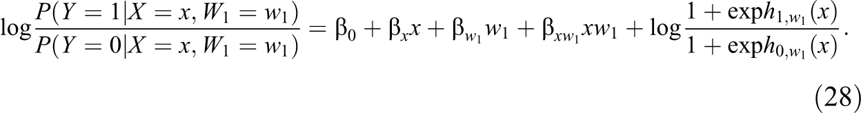
with the expression of
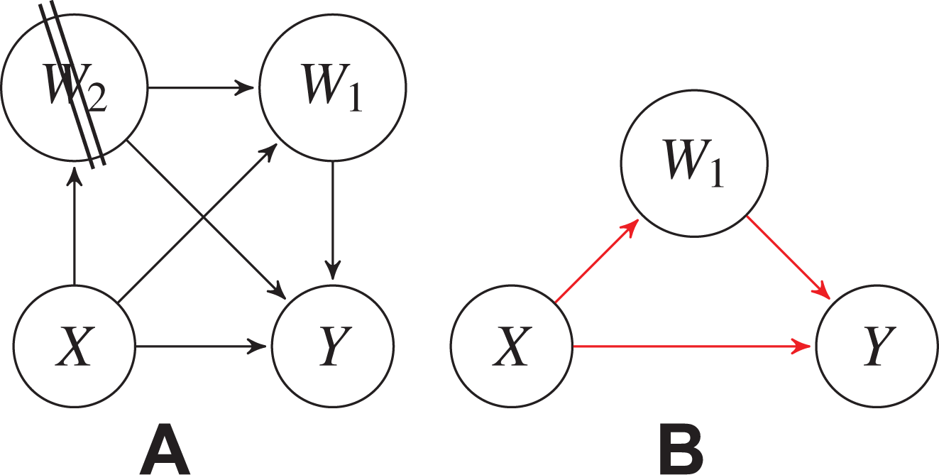
(A) Marginalization over the outer mediator W 2 and (B) quantifying the parameters (in red the parameters that change).
Causal Interpretation of Total, Direct, and Indirect Effects
In the counterfactual framework, many approaches exist to mediation analysis, and a review is in Huber (2019). In a single-mediator context, VanderWeele and Vansteelandt (2010) define the counterfactual notion of direct and indirect effects when the outcome is binary, thereby focusing on the log odds scale. Within a regression analysis context with a continuous mediator, the authors present an approximated parametric formulation of the effects that holds under the rare outcome assumption of Y. Valeri and VanderWeele (2013) address the same problem when also the mediator is binary, again modeled under the rare outcome assumption. It is therefore worth to explore the links existing between the effects introduced here and these causal effects defined in a formal counterfactual framework. Since the latter are contrasts expressed, possibly after a logarithmic transformation, by a difference, this parallel holds for X binary. Notice that, differently from the above cited approaches, we here present a decomposition based on the exact formulation of the effects on the log odds scale.
Under the assumption that the recursive system of equation is structural in the sense of Pearl (2009, chap. 7), one can give the total effect and some of its components a causal interpretation. To say that the recursive system of equations is structural implies that the DAG is a causal graph that satisfies a set of axioms, namely, composition, effectiveness, and reversibility (see also Steen and Vansteelandt 2018).
With a single binary mediator, a parallelism between the structural definition of a DAG and the sequential ignorability assumption of Imai, Keele, and Yamamoto (2010) exists (see Pearl 2012; Shpitser and VanderWeele 2011). Under the assumption of no unmeasured counfounder of the treatment–outcome relationship, possibly after conditioning on a set of pretreatment covariates C, the total effect of X on Y here presented corresponds to the total causal effect as defined by VanderWeele and Vansteelandt (2010). Similarly, assuming that there are no unobserved confounders of the treatment–outcome relationship, possibly after conditioning on a set of pretreatment covariates C, and no unmeasured confounders of the mediator-outcome relationship, after conditioning on the treatment X and possibly some pretreatment covariates C, the direct effect can be seen as the controlled direct effect (VanderWeele and Vansteelandt 2010) after an external intervention to fix
When multiple causally ordered mediators are present, several possible effects are of interest (see Daniel et al. 2015; Steen et al. 2017). However, in this case, the definition of natural direct and indirect effects is more cumbersome, and sometimes effects of interest are nonidentifiable (see, e.g., the situation described in Avin, Shpitser, and Pearl [2005]). Again, if no unobserved confounders exist, some parallelisms continue to hold. As an instance, the direct effect can be seen as the controlled direct effect of X on Y after an external intervention to fix the mediators
Conclusions
Logistic regression is by far the most used model for a binary response. Further than in a mediation context, the models here proposed may arise in longitudinal studies with a binary outcome measured at different occasions.
With reference to a single mediator, we have proposed a novel decomposition of the total effect into direct and indirect effects that is more appropriate for the nonlinear case and that, under certain conditions, reduces to the classical definition in the linear case. Additionally, this decomposition overcomes the issue of unequal variance when fitting two nested models. As an illustrative example, we have reanalyzed data based on an encouragement program to stimulate students’ attitude to visit museums. We have shown how the decomposition of the total effect could avoid erroneous conclusions on the direct and indirect effects and provides additional information that cannot be found by just looking at the results of the separate regressions analysis. Although the total, direct, and indirect effects are all positive, a substantial residual effect, possibly due to a large interaction coefficient, hinders the interpretation in terms of proportion mediated.
Additional important results concern the extension of the definitions to the multiple mediator context. Repeated use of the decomposition of the total effect allows to address complex issues like quantifying the total, direct, and indirect effects when a subset of mediators are marginalized over. Links to the causal effects have also been established.
Supplemental Material
Supplemental Material, sj-docx-1-smr-10.1177_00491241211031260 - Path Analysis for Binary Random Variables
Supplemental Material, sj-docx-1-smr-10.1177_00491241211031260 for Path Analysis for Binary Random Variables by Martina Raggi, Elena Stanghellini and Marco Doretti in Sociological Methods & Research
Supplemental Material
Supplemental Material, sj-r-1-smr-10.1177_00491241211031260 - Path Analysis for Binary Random Variables
Supplemental Material, sj-r-1-smr-10.1177_00491241211031260 for Path Analysis for Binary Random Variables by Martina Raggi, Elena Stanghellini and Marco Doretti in Sociological Methods & Research
Supplemental Material
Supplemental Material, sj-r-2-smr-10.1177_00491241211031260 - Path Analysis for Binary Random Variables
Supplemental Material, sj-r-2-smr-10.1177_00491241211031260 for Path Analysis for Binary Random Variables by Martina Raggi, Elena Stanghellini and Marco Doretti in Sociological Methods & Research
Footnotes
Authors note
The author Martina Raggi is also affiliated with Université de Paris, INSERM U1153, Epidemiology of Ageing and Neurodegenerative diseases Paris, France
Declaration of Conflicting Interests
The author(s) declared no potential conflicts of interest with respect to the research, authorship, and/or publication of this article.
Funding
The author(s) received no financial support for the research, authorship, and/or publication of this article.
Supplemental Material
The supplemental material for this article is available online.
References
Supplementary Material
Please find the following supplemental material available below.
For Open Access articles published under a Creative Commons License, all supplemental material carries the same license as the article it is associated with.
For non-Open Access articles published, all supplemental material carries a non-exclusive license, and permission requests for re-use of supplemental material or any part of supplemental material shall be sent directly to the copyright owner as specified in the copyright notice associated with the article.