Re-Evaluating Sexual Violence Prevention Through Bystander Education

Abstract

Recently, there has been a call for more advanced analytic techniques in violence against women research, particularly in community interventions that use longitudinal designs. The current study re-evaluates experimental evaluation data from a sexual violence bystander intervention program. Using an exploratory latent growth curve approach, we were able to model the longitudinal growth trajectories of individual participants over the course of the entire study. Although the results largely confirm the original evaluation findings, the latent growth curve approach better fits the demands of “messy” data (e.g., missing data, varying number of time points per participant, and unequal time spacing within and between participants) that are frequently obtained during a community-based intervention. The benefits of modern statistical techniques to practitioners and researchers in the field of sexual violence prevention, and violence against women more generally, are further discussed.

Keywords

rape prevention latent growth curve analysis experimental evaluation longitudinal design interventions

Epidemiological data estimate that one in five women experiences a sexual assault in her lifetime, potentially leading to myriad detrimental effects on psychological, physical, social, health, and behavioral outcomes (Black et al., 2011; Martin, Macy, & Young, 2011). Given the high rate of sexual victimization and the impact of this traumatic event, there has been growing attention on the development, implementation, and evaluation of sexual assault prevention programs (see Gidycz, Orchowski, & Edwards, 2011; Lonsway et al., 2009; Vladutiu, Martin, & Macy, 2011; The White House Council on Women and Girls, 2014). To date, however, there are few experimental evaluations of these programs, and although they are becoming increasingly common (e.g., Banyard, Moynihan, & Plante, 2007; Foubert, 2000; Gidycz, Orchowski, & Berkowitz, 2011; Orchowski, Gidycz, & Raffle, 2008; Senn et al., 2013; Senn, Gee, & Thake, 2011; Taylor, Stein, Mumford, & Woods, 2013), these evaluations have yet to use holistic longitudinal models for data analysis, even when their design includes longitudinal components.¹ More specifically, these previous evaluations used mean difference frameworks (e.g., repeated-measure MANCOVA) to examine whether intervention groups systematically differ from control groups. This technique is certainly appropriate. However, recent developments in longitudinal modeling have highlighted advantages of using more complex techniques such as hierarchical linear and structural equation models that more closely link practitioner conceptions of individual change to the modeling approach (Dijkers, 2012; Locascio & Atri, 2011). The primary focus of the current study is to explore the advantages of emerging approaches to longitudinal analysis by re-examining data from one of the first experimental evaluations of a sexual violence bystander intervention program, “Rape Prevention Through Bystander Education at a Northeastern State University, 2002-2004” (Banyard, Plante, & Moynihan, 2008). Using growth curve modeling, we attempt to illustrate a more holistic understanding of change over time in contexts with “messy” data (Locascio & Atri, 2011), while attending to the call for advanced analytic techniques within violence against women research (see Campbell, 2011; Swartout, Swartout, & White, 2011).

In discussing sexual violence intervention programs, the terms “prevention program,” “risk reduction program,” and “educational program” may be used interchangeably. However, they are implicative of different interventions and underlying philosophies. These different philosophies, whether explicit or not, inform programmatic decisions on whom to target, through what strategies, and with what dosage or intensity. With regard to the target audience, programs may target women as potential victims (e.g., Orchowski et al., 2008) or, although far less common (Lonsway et al., 2009), men as potential perpetrators (e.g., Gidycz, Orchowski, & Berkowitz, 2011). Strategies may emphasize increased knowledge and altered attitudes, or extend into behavior change (see Lonsway et al., 2009, for a review). Regarding dosage, programs may be provided in “one shot” (e.g., Foubert, 2000) or a series of sessions (e.g., Coker et al., 2011) varying in the length of each session.

Variations in the target audience, strategies used, and dosage may significantly affect the program’s ability to achieve its desired outcomes. Yet with all these variations in programming, few sexual assault prevention programs have been empirically evaluated, and even fewer have used an experimental design with random assignment into the treatment and control groups. Although random assignment in these situations can be challenging, it is invaluable as it attempts to evenly distribute any individual characteristics or experiences among participants that might confound the results (Singleton & Straits, 2010), minimizing alternative explanations for relatedness among the independent and dependent variable(s). Studies that have used experimental evaluations of sexual assault intervention programs are promising. Programs for men have documented greater changes in rape myth acceptance, the likelihood of committing rape, and perceptions of sexually aggressive behavior in treatment groups as compared with control groups (Foubert, 2000; Gidycz, Orchowski, & Berkowitz, 2011); programs for women have documented effective change for self-protective behaviors, assertive sexual communication, and self-defense strategies for treatment groups as compared with control groups (Orchowski et al., 2008); and mixed gender programs have documented reductions in reported sexual violence victimization involving peers or dating partners for treatment groups as compared with control groups (Taylor et al., 2013).

Recently, Banyard and colleagues (Banyard et al., 2007; Banyard, Plante, & Moynihan, 2005) conducted an experimental evaluation of a bystander intervention program. The bystander, as conceptualized by Banyard et al. (Banyard, Plante, & Moynihan, 2005), exists not as a victim or perpetrator, but as a separate individual who can intervene in situations that involve sexual violence. By including and emphasizing the role of the bystander, these types of programs move beyond the individual and focus on the whole community; all community members have a specific role in preventing sexual violence through challenging social norms and intervening in questionable situations (Banyard et al., 2007; Banyard, Plante, & Moynihan, 2005; Lonsway et al., 2009). Banyard and colleagues (Banyard, Plante, & Moynihan, 2005) evaluated the impact of a “one-shot” program paired with a booster and a series of sessions (i.e., three sessions) paired with a booster, to no program intervention at all (i.e., control group). Repeated-measures MANCOVA, MANOVA, and post hoc paired-sample t tests found the program to be effective. From pretest to posttest, the treatment groups had significantly greater difference scores as compared with the control group on all measures; the program with higher dosage (i.e., the three session group) had significantly greater difference scores as compared with the “one-shot” program on knowledge, bystander attitudes, and rape myth acceptance. In addition, the recorded changes were significant in the expected direction for both treatment groups from pretest to posttest and from pretest to the 2-month follow-up. Due to research and analytic design constraints (i.e., the wave design resulting in missing data on half of the participants for the 4-month follow-up and 12-month follow-up and more women presented for the 12-month follow-up), the authors described their assessment of the 4-month and 12-month follow-up data as exploratory; they conducted paired-sample t tests to examine changes in means scores from pretest to each of these follow-up time points and found similar trends.

The overall analytic design of the bystander intervention program (Banyard et al., 2007; Banyard, Plante, & Moynihan, 2005) provided evidence of its effectiveness through a series of statistical tests, including repeated-measures MANCOVA and paired-sample t tests. This analytic approach generally works well for longitudinal research designs that are well-balanced, in that they have the “same, relatively few, and usually evenly spaced time points for each subject, with no missing values” (Locascio & Atri, 2011, p. 338). However, although many community interventions and corresponding longitudinal evaluations are well-balanced in design, they are subject to high rates of participant attrition in practice, resulting in “messy” data with missing values, varying numbers of time points per participant, and unequal time spacing within and between participants (see Gustavson, von Soest, Karevold, & Røysamb, 2012, for a discussion of attrition rates in longitudinal designs; Locascio & Atri, 2011).

Latent growth curve analysis provides an alternative analytic design well-fitted to handle the demands of “messy” data from community interventions. This approach has several key advantages over more traditional analytic approaches, such as MANCOVA and paired-sample t tests (see Locascio & Atri, 2011, for a discussion of these different approaches). First, with regard to handling missing data, latent growth curve modeling is much more flexible (Krueger & Tian, 2004). This is because the maximum likelihood estimation used in most latent growth curve analysis is able to include all observations and provide unbiased estimates when data are missing at random (Enders, 2001). This can be contrasted to most implementations of MANCOVA approaches that use listwise deletion, thereby losing information from every individual who has missing data. In the current data set, each wave of data collection included a single long-term follow-up at either 4 or 12 months, in addition to data collection at pre, post, and 2 months. For this reason, the primary analysis in the Banyard et al.’s (Banyard, Plante, & Moynihan, 2005) article included only the first three time points (pre, post, 2 months). Using latent growth curves, we can estimate longitudinal change across all time points in the primary model. Therefore, the estimates of intervention effect size should be more informative about long-term change in the intervention outcomes.

Second, latent growth curve model changes at the individual level by allowing each individual’s change to be estimated separately using a random-effects approach (Locascio & Atri, 2011). This approach more accurately reflects common theoretical conceptualizations of individual change in that each individual changes at some rate; we observe this distribution of individual change and look for differences in these distributions between intervention and control groups to see whether group membership has affected the average rate of change. This approach can even be used to detect latent classes of participants with similar change trajectories within each given class, but different across classes (Locascio & Atri, 2011). This is in contrast to repeated-measure MANCOVA where individuals within groups are assumed to follow the same trajectory using a fixed-effect approach.

Third, the latent growth model approach is more flexible in modeling non-linear change (see Locascio & Atri, 2011, for a discussion of linear vs. non-linear change). Descriptive statistics in Banyard et al.’s (Banyard, Plante, & Moynihan, 2005) analysis suggest decay in intervention effects over time, as decay of intervention effects are common in social science intervention research (Allen & Reynolds, 1993; Arthur, Bennett, Stanush, & McNelly, 1998; Gidycz, Orchowski, & Berkowitz, 2011; Orchowski et al., 2008). Accordingly, the participants likely exhibited a non-linear change over time. An exploratory latent growth curve model is ideal for reflecting these patterns of change as it does not assume or attempt to fit an a priori change trajectory and instead attempts to provide the most accurate model of the data (unlike confirmatory latent growth curve modeling; see Grimm, Steele, Ram, & Nesselroade, 2013).

Like many community interventions with longitudinal evaluation designs, the Banyard et al. (Banyard et al., 2007; Banyard, Plante, & Moynihan, 2005) study is an ideal candidate for latent growth curve modeling due to its “messy” data. Specifically, the study had missing data: planned missing data on half of the participants at the 4-month follow-up and 12-month follow-up (i.e., as a result of the wave design) and unplanned missing data due to individuals not completing their assigned long-term follow-up surveys (see Banyard, Plante, & Moynihan, 2005, for specific rates of attrition); a varying number of time points per participant: There were a total of five data collection time points, although the number of data collection time points completed by any individual varied; and unequal time spacing within and between subjects: Some participants had their final assessment at 4 months, whereas others completed theirs at 12 months. For these reasons, we believe that a longitudinal model using exploratory latent growth curves should be applied to the bystander intervention program data to examine how change happens within this context, such as if participant scores peak, if they level out, and if their final level is below or at their original scores. An exploratory latent growth model approach that does not introduce post hoc comparisons between individual time points² will allow us to see all the time points in a single model, and then examine whether the results of the latent growth curve approach align with and/or build on the findings of prior analyses using more traditional methods. In doing so, the current study attempts to answer the recent call for more advanced analytic techniques in evaluations of community interventions (see Campbell, 2011; Swartout et al., 2011) and extends this conversation by showcasing the benefits of latent growth curve modeling via the following research aims: (a) demonstrate how the longitudinal question of how individuals change over time can be modeled directly with exploratory latent growth modeling and how intervention effects can be estimated through the use of a multiple group modeling, and (b) identify and discuss the benefits of this approach for the current analysis and for future research and evaluation using longitudinal designs in community settings.

Method

Participants

The data used in this study were collected by Banyard et al. (Banyard, Plante, & Moynihan, 2005) and were obtained through the National Archive of Criminal Justice Data of the Inter-University Consortium for Political and Social Research (ICPSR). A total of 389 undergraduates were selected for the study across two waves (multiple waves were used due to constraints of the project and academic calendar; see Banyard et al., 2007; Banyard, Plante, & Moynihan, 2005, for a complete description of recruitment and selection procedures, including inclusion criteria). Data were missing for all time points on the knowledge scale, rape myth acceptance scale, and bystander efficacy scale for three, five, and two individuals, respectively, and these individuals were removed from the data set, yielding final sample sizes of N = 386 for the knowledge model, N = 384 for the rape myth acceptance model, and N = 387 for the bystander efficacy model. Banyard and colleagues (Banyard et al., 2007; Banyard, Plante, & Moynihan, 2005) provided details on participant demographics, but briefly the sample was 55.8% female and 90.4% White, and averaged 19.4 years old.

Procedure

Participants were randomly assigned to one of three groups across two waves: a control group, Treatment Group 1, or Treatment Group 2. The control group did not receive a prevention program intervention. Participants in Treatment Group 1 attended one 90-min prevention program session on sexual violence and the role of community members, followed by a booster program 2 months later. Participants in the Treatment Group 2 attended three 90-min prevention program sessions in a week, consisting of expanded content from the single-session format, followed by a booster program 2 months later (see Banyard et al., 2007; Banyard, Plante, & Moynihan, 2005, for details on the prevention programs). Data were collected at five time points measuring participant knowledge, attitudes, and perceived role of the bystander in relation to sexual violence, although no participant was measured at all five occasions. All participants completed a pretest, posttest, and 2-month follow-up questionnaire; Wave 1 participants completed the 4-month follow-up questionnaire; and Wave 2 participants completed the 12-month follow-up questionnaire.

Measures

Banyard et al. (Banyard, Plante, & Moynihan, 2005) used previously validated measures and created new measures for their experimental evaluation (see Banyard, Plante, & Moynihan, 2005, or all measures). The same set of measures were used at each data collection time point (i.e., pretest, posttest, 2-month follow-up, 4-month follow-up, and 12-month follow-up). The current study examines three of the scales used in the original questionnaire: knowledge about sexual violence, rape myth acceptance, and bystander efficacy.

Knowledge about sexual violence

Knowledge gained during the prevention program as an outcome measure was assessed using a 10-item scale. Via multiple-choice and short-answer items, participants were asked to identify what qualifies as sexual violence, rates of sexual violence and false reports of sexual assault, the role of consent and drug use during sexual encounters, and the role of a bystander. Higher scores on this scale indicated greater knowledge (i.e., a greater score is desired; see Banyard et al., 2007; Banyard, Plante, & Moynihan,., 2005). Banyard et al. (2007) found Cronbach’s α = .84 (M = 17.04, SD = 6.12 with a range of 0 to 31).

Rape myth acceptance

Rape myth acceptance as an outcome measure was assessed using the college date rape attitude survey (Lanier & Elliot, 1997, as referenced in Banyard et al., 2007; Banyard, Plante, & Moynihan, 2005). Participants were asked to endorse statements such as “males and females should share the expenses of a date” or “if a woman dresses in a sexy dress she is asking for sex” on a scale from 1 to 5 (see Banyard, Plante, & Moynihan, 2005, for the full measure). Higher scores on this 20-item scale indicate greater disagreement with rape myths (i.e., a greater score is desired). Banyard and colleagues (2007) found Cronbach’s α = .92 (M = 76.59, SD = 25.33 with a range from 26 to 98).

Bystander efficacy

Finally, the role of the bystander as an outcome measure was assessed using a 14-item bystander efficacy scale developed and pilot tested by Banyard, Plante, & Moynihan,. (2005). In Banyard et al.’s (Banyard et al., 2007; Banyard, Plante, & Moynihan, 2005) study, participants indicated how confident they were in performing 14 different bystander behaviors (e.g., “express my discomfort if someone makes a joke about a woman’s body”) on a scale of 0 “can’t do” to 100 “very certain can do.” The average of these 14 items was subtracted from 100 yielding a score of perceived ineffectiveness (i.e., a low score is desired). Banyard et al. (2007) found a Cronbach’s alpha of .87 (M = 20.55, SD = 14.19 with a range of 0 to 92.86). However, in the current study, we did not invert this score (i.e., subtract the score from 100) in an effort to ease interpretation (i.e., have all dependent variables with higher scores being more desirable).

Analysis

Raw scores for all participants on the scales of interest (i.e., 10-item knowledge assessment, 20-item date rape myth acceptance efficacy, and 14-item bystander efficacy assessment) across the five time points were converted into mean scores as described above. Mplus (L. K. Muthén & Muthén, 1998-2011) was used to model three separate series of multi-group (control vs. Treatment 1 vs. Treatment 2) latent growth curves for each dependent variable (i.e., knowledge, rape myth acceptance, and bystander efficacy) to determine the model that most appropriately captured the pattern of change over time, in consideration of the effect of group (see Bollen & Curran, 2005). The same analytic procedure was used for each series of latent growth curves. All five time points (i.e., pretest, posttest, 2-month follow-up, 4-month follow-up, and 12-month follow-up) were included in each model using maximum likelihood estimation (B. Muthén, Jo, & Brown, 2003; L. K. Muthén & Muthén, 1998-2011).

Before fitting any models, each outcome was examined to explore for patterns of missing data using Little’s (1988) test for missing completely at random (MCAR). This test examines whether the data can be considered MCAR. A non-significant result suggests data could be considered missing at random, and no further adjustment is needed when using maximum likelihood estimation.³ Following assessment of missing data, models were then fit using an iterative step approach starting with a no-growth model, moving to a latent basis model, and systematically freeing parameters to examine for group differences across control and experimental groups. In contrast to a traditional latent linear latent growth model, this exploratory approach was selected as it does not assume or attempt to test a specific hypothesis or theory of change over time. Rather, the latent basis model allows the shape of the curve to be estimated from the data. The first basis coefficient is set to 0 (i.e., the basis coefficient at the pretest is 0), and the last basis coefficient is set to 1 (i.e., the basis coefficient at the 12-month follow-up is 1), whereas the three basis coefficients in between are estimated (i.e., the basis coefficients for posttest, 2-month follow-up, and 4-month follow-up). The basis coefficients can then be interpreted in terms of how much growth occurred between each observation in relation to how much change occurred over the course of the study. A latent basis model is appropriate as we did not expect linear change due to the typical attrition of intervention effects for psycho-social-educational interventions (Allen & Reynolds, 1993; Arthur et al., 1998). Accordingly, growth is not assumed to change in a linear manner. Figure 1 provides the path diagram for the latent basis model for a single group.

Figure 1.

Path diagram for a single group.

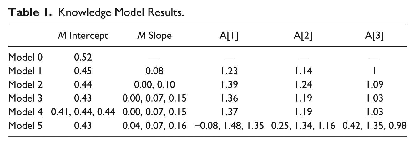
For Model 0, we used a no-growth model that only included an intercept with all parameters constrained across groups. For Model 1, a latent basis model was used with the slope being held constant across groups. For Model 2, the mean slope of the control group was freed allowing to test the change in control versus both experimental groups. For Model 3, mean slopes were freed across all groups to test the difference between slope means for Treatment 1 and Treatment 2. Model 4 allowed the intercepts to vary across groups. Model 5 allowed each basis coefficient for posttest, 2 months, 4 months to vary across all groups. Chi-square difference tests (Bentler & Bonett, 1980) were used to determine the best fitting model for each outcome measure of interest (i.e., knowledge, rape myth acceptance, and bystander efficacy). Global fit indices, including the root mean square error of approximation (RMSEA), comparative fit index (CFI), and Tucker–Lewis index (TLI), were also examined to assess for absolute fit.⁴

Results

Model results for knowledge, date rape myth acceptance, and bystander efficacy are presented in Tables 1 through 3, respectively. A non-significant negative slope variance in all models suggested that there was no remaining variance in the rate at which participants changed after accounting for group membership. Accordingly, the slope variance parameter was set to zero for all models, and, because of this constraint, the intercept and slope covariance was required to be constrained to zero. Results of Little’s (1988) test for MCAR suggested that knowledge, rape myth acceptance, and bystander efficacy could be considered MCAR (p = .135, p = .956, and p = .307, respectively).

Table 1.

Knowledge Model Results.

	M Intercept	M Slope	A[1]	A[2]	A[3]
Model 0	0.52	—	—	—	—
Model 1	0.45	0.08	1.23	1.14	1
Model 2	0.44	0.00, 0.10	1.39	1.24	1.09
Model 3	0.43	0.00, 0.07, 0.15	1.36	1.19	1.03
Model 4	0.41, 0.44, 0.44	0.00, 0.07, 0.15	1.37	1.19	1.03
Model 5	0.43	0.04, 0.07, 0.16	−0.08, 1.48, 1.35	0.25, 1.34, 1.16	0.42, 1.35, 0.98

Table 2.

Date Rape Myth Acceptance Model Results.

	M Intercept	M Slope	A[1]	A[2]	A[3]
Model 0	9.87		—	—	—
Model 1	3.65	0.24	0.76	1.02	1
Model 2	3.65	0.12, 0.30	0.77	1.07	1
Model 3	3.64	0.12, 0.28, 0.31	0.78	1.08	1.02
Model 4	3.64, 3.68, 3.60	0.12, 0.26, 0.33	0.81	1.08	1.03
Model 5	3.65	0.09, 0.37, 0.27	0.89, 0.52, 1.06	1.42, 0.84, 1.18	1.09, 0.79, 1.16

Table 3.

Bystander Efficacy Model Results.

	M Intercept	M Slope	A[1]	A[2]	A[3]
Model 0	85.33		—	—	—
Model 1	81.58	3.32	1.58	1.22	0.99
Model 2	79.53	0.16, 6.50	1.35	1.15	1.04
Model 3	79.4	0.18, 5.74, 7.41	1.34	1.14	1.04
Model 4	79.35, 79.41, 79.42	0.18, 5.74, 7.40	1.34	1.14	1.04
Model 5	79.41	0.07, 6.01, 7.08	7.60, 1.23, 1.42	3.01, 1.16, 1.152	−11.00, 1.04, 1.05

Knowledge About Sexual Violence

For knowledge (Table 1), the no-growth model (Model 0) had significant misfit, χ²(38) = 386.21, p < .001, and poor fit on other indices, RMSEA = 0.266, 90% confidence interval (CI) = [0.24, 0.29], CFI = 0.339, TLI = 0.531. The fully constrained latent basis model (Model 1) significantly improved fit, Δχ²(4) = 137.78, p < .001, suggesting change occurred during the course of the study. However, Model 1 still showed significant misfit, χ²(34) = 248.44, p < .001, and poor fit on other indices, RMSEA = 0.221, 90% CI = [0.20, 0.25], CFI = 0.593, TLI = 0.677. The model with the mean slope freed across control and experimental groups (Model 2) significantly improved fit, Δχ²(1) = 119.76, p < .001, indicating that experimental groups had a significantly different mean slope (M = 0.10) compared with the control group (M = 0.00). However, Model 2 still showed significant misfit, χ²(33) = 128.68, p < .001, and poor fit on other indices, RMSEA = 0.150, 90% CI = [0.12, 0.18], CFI = 0.818, TLI = 0.851. The model with all slope means freed (Model 3) again significantly increased fit, Δχ²(1) = 71.18, p < .001, indicating that the mean slope of Treatment 1 (M = 0.07) significantly differed from the slope of Treatment 2 (M = 0.15). Model 3 showed acceptable fit on other indices, RMSEA = 0.078, 90% CI = [0.04, 0.11], CFI = 0.951, TLI = 0.949, although still showing significant misfit, χ²(32) = 57.50, p = .004. Model 4 did not show a significant increase in fit suggesting that the intercepts did not vary across groups Δχ²(2) = 1.53, p = .466. The non-significant increase in fit when freeing the intercepts suggests that these groups did not show significant differences on the outcome measure at the pretest. Nor did Model 5 (basis coefficients freed) show significant increase over Model 3, Δχ²(6) = 3.92, p = .488, suggesting that these coefficients did not vary across groups. A non-significant increase in the model fit when freeing the basis coefficients suggests that, although participants may change at different rates, the general pattern of change over the course of the study did not differ across groups (i.e., some increase with decay toward later time points). Accordingly, Model 3 was chosen as our final model. Basis coefficients (Table 1) for this model indicated that scores tended to peak at posttest (A[1] = 1.36) and stay slightly elevated during the 2- and 4-month follow-ups (A[2] = 1.19, A[3] = 1.03) compared with the final scores (i.e., at 12 months). Figure 2a shows the mean trajectory for each group on top of a spaghetti plot of a 30% random sampling of all individual trajectories. As shown, this figure displays the significantly higher slope of Treatment 2 versus Treatment 1 and Treatment 1 versus the control group. In sum, the more intense the initial intervention program, the greater the change in knowledge of sexual assault (i.e., the three-session program had a significantly greater slope than the one-session program; the one-session program had a significantly greater slope than the control).

Figure 2.

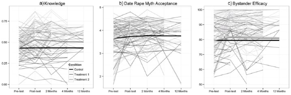
Individual and predicted growth by experimental group.

Rape Myth Acceptance

The no-growth model for rape myth acceptance (Table 2) had significant misfit, χ²(38) = 116.47, p < .001. Model 1 significantly improved fit, Δχ²(4) = 55.49, p < .001, but continued to show significant misfit, χ²(34) = 61.97, p = .003, and moderate fit on other indices, RMSEA = 0.078, 90% CI = [0.05, 0.11], CFI = 0.905, TLI = 0.924. Freeing the mean slope for the control group significantly improved fit, Δχ²(1) = 13.24, p < .001, again suggesting that the control group had a different mean slope (M = 0.12) as compared with the experimental groups (M = 0.30). Other indices also improved in Model 2, RMSEA = 0.059, 90% CI = [0.01, 0.09], CFI = 0.948, TLI = 0.958, although this model still had significant misfit, χ²(33) = 47.73, p = .047. For Model 3, freeing the experimental group mean slopes did not significantly improve fit, Δχ²(1) = 0.14, p = .704, indicating the mean slope for Treatment 1 (M = 0.28) did not significantly differ from Treatment 2 (M = 0.31). Compared with Model 2, neither the intercept free, Δχ²(2) = 1.38, p = .501, nor the basis coefficient free, Δχ²(6) = 0.89, p = .893, models significantly improved fit. Accordingly, Model 2 was chosen as the final model. Basis coefficients for this model indicated that scores peaked at 2-month follow-up (A[2] = 1.07). Figure 2b displays the predicted model on top of a 30% random sampling of all individual trajectories for rape myth acceptance. In sum, the intervention program significantly decreased rape myth acceptance among participants as compared with the control group. The intensity of the initial program provided (three sessions vs. one session) did not make a statistically significant difference in rape myth acceptance.

Bystander Efficacy

The no-growth model for bystander efficacy (Table 3) also showed significant misfit, χ²(38) = 202.24, p < .001. Model 1 significantly improved fit, Δχ²(4) = 65.32, p < .001, although this model still had significant misfit, χ²(34) = 136.91, p < .001, and showed poor overall fit, RMSEA = 0.153, 90% CI = [0.13, 0.21], CFI = 0.874, TLI = 0.900. Model 2 again significantly increased fit, Δχ²(4) = 72.314, p < .001, indicating the experimental groups had a significantly higher mean slope (M = 6.50) compared with the control group (M = 0.16). Model 2 also showed significant misfit, χ²(33) = 64.60, p < .001, and moderate fit on other indices, RMSEA = 0.086, 90% CI = [0.05, 0.12], CFI = 0.961, TLI = 0.968. Model 3 also significantly improved fit, Δχ²(4) = 4.23, p < .001, suggesting Treatment 2, the group that attended three sessions, had a significantly higher mean slope (M = 7.40) compared with Treatment 1 (M = 5.74), the group that attended a single session. Finally, neither Model 4, Δχ²(2) = 0.00, p = .999, nor Model 5, Δχ²(6) = 2.75, p = .840, significantly improved fit leaving Model 3 as our final model. For bystander efficacy, the basis coefficients indicated that scores peaked at posttest (A[1] = 1.34). Figure 2c displays the predicted model on top of a 30% random sampling of all individual trajectories for bystander efficacy. Similar to the knowledge domain, the more intense the initial intervention program, the greater the change in knowledge of sexual assault (i.e., the three-session program had a significantly greater slope than the one-session program; the one-session program had a significantly greater slope than the control).

Discussion

Banyard et al. (Banyard et al., 2007; Banyard, Plante, & Moynihan, 2005) found their bystander intervention program for sexual assault prevention to be effective across the domains of knowledge, attitudes, and the role of bystanders by analyzing between-group mean difference scores. However, like most community interventions, this study was conducted in a context that resulted in missing data, a varying number of time points per participant, and unequal time spacing within and between participants. Therefore, the purpose of the current study was to re-analyze these data with a latent growth curve modeling approach, which is better suited to meet the demands of “messy” data, to see whether the original findings could be corroborated and to identity the benefits of using this advanced analytic technique in evaluating the impact of longitudinal community interventions.

As demonstrated in its initial evaluation (Banyard et al., 2007; Banyard, Plante, & Moynihan,., 2005) and confirmed in the present study, the bystander intervention program was successful in significantly affecting participants’ knowledge of sexual violence, date rape myth acceptance, and bystander efficacy over time. Participants in both treatment groups knew more about sexual violence, were less likely to endorse rape myths, and had a greater sense of efficacy intervening as a bystander as compared with individuals in the control group. In addition, participants who received the more intense initial intervention (i.e., three 90-min sessions) knew more about sexual violence and had a greater sense of efficacy intervening as a bystander as compared with individuals who received the less intense initial intervention (i.e., one 90-min session). The growth curve modeling corroborated the findings of Banyard et al. (Banyard et al., 2007; Banyard, Plante, & Moynihan,., 2005), demonstrating that no information was lost in creating a single parsimonious model for each dependent variable of interest, as opposed to running a series of mean and difference score comparisons. In addition, new information was gained as a result of this analytical technique. By modeling the average individual’s trajectory in each group (i.e., control, Treatment Group 1, and Treatment Group 2) over time, we can conclude that the average individual in a treatment group was not just different from the average individual in the control group at the posttest, or at the 2-month follow-up. Rather, their predicted change trajectory (i.e., slope) in the desired outcomes from pretest to the 12-month follow-up was significantly different.

Finally, latent growth curve analysis was able to present the findings in a new way that more explicitly showcased how the change trajectories over time differed across the outcome variables of interest. As mentioned, dosage affected the effect of the intervention. Specifically, the program in either form (one or three 90-min sessions) was always better than the control in affecting the variables of interest. However, the more intensive program was successful in producing significantly more growth for knowledge and bystander efficacy related to sexual violence (compared with the less intensive intervention), whereas it had no greater impact on rape myth acceptance through the average individual’s growth trajectory. This insight was possible using multi-group latent growth curve modeling because we were able to test directly whether the overall growth of each group significantly varied from the others. This differs from Banyard, Plante, & Moynihan’s (2005) original findings that only examined the change in each group separately. In addition, this approach suggested that the booster (administered at 2 months) may have had a greater impact on date rape myth acceptance and bystander efficacy, as scores peaked at this data collection point, whereas the knowledge outcome scores peaked at the posttest.

Given that the specific dosage for any intervention program should be informed by the desired outcomes, these findings suggest that if a change in knowledge alone is desired, an initial intensive program may be sufficient, with no booster required; if a change in attitude/rape myth acceptance alone is desired, a less intensive initial program paired with a booster may be required; if a change in bystander efficacy/intent to act alone is desired, an initial intensive program paired with a booster may be necessary.⁵ Although these same findings may have been able to be gleaned from the original analyses, latent growth curve analysis packages them in a different way by modeling the growth trajectory for the average individual across the course of the study. This procedure more closely aligns with the research question and practitioner conceptions of individual change, providing a more parsimonious and comprehensive model of the change process. As such, researchers and practitioners are better able to identity when their intervention has its greatest impact (i.e., peak) and then use this information to adjust future programming to achieve desired results.⁶

Beyond confirming and re-packaging the original analyses to improve interpretability and immediate utility, the current study was able to showcase two of the other key benefits of latent growth curve modeling. As discussed, this approach is ideal for handling “messy” data. More traditional methods, such as repeated-measure ANOVA or MANCOVA, are sensitive to data that are not well-balanced, with the same number of similarly spaced time points across participants, and frequently eliminate all data for participants with even a single missing value (Locascio & Atri, 2011). These approaches are not well-suited for community settings in which there are a multitude of variables that are not easily controlled by the researcher, including high rates of attrition among participants over time. Rather than removing all data associated with a participating with just one missing value, latent growth curve analysis uses maximum likelihood estimation to include all observations, even for those participants with some missing values, to provide unbiased estimates (i.e., when data are missing at random; Enders, 2001). This provides a working solution for researchers working in communities with data that are incomplete and situation in which listwise deletion (i.e., removing all cases with any missing values) and/or imputation are not viable solutions.

A second key benefit of the exploratory latent growth curve approach is that the analysis does not assume or try to test a specific theory of change, but rather builds the model that most accurately represents the data. This can be particularly useful for researchers and practitioners who are focused on trying to understand change as it happens on the ground. For example, researchers can use exploratory latent growth curve analysis to model the impact of pilot intervention programs and then partner with practitioners to use the findings for program revisions prior to scaling up (i.e., expanding the intervention beyond the initial pilot program). Alternatively, researchers may choose to use a confirmatory latent growth curve approach to test whether the intervention’s expected change trajectory, for example, an early change in attitudes followed by a change in behavior, is realized. Through these means, researchers and practitioners can vary intervention program dosage and then examine its effects on change over time. This process has the potential to yield detailed information on what specific dosage is required to achieve desired intervention outcomes.

Limitations

Although this study corroborates the findings of Banyard, Plante, & Moynihan’s (2005) original analysis and provides an alternative analytical framework producing new insight for studying and facilitating longitudinal change in sexual violence prevention program initiatives, it does have important limitations. The current study is based on archival data from a single university collected from 2002 to 2004; this may limit the generalizability of the substantive findings. Also, the stepwise approach chosen in the current study (i.e., starting with a fully constrained model across groups and freeing parameters) was only one approach to take in the modeling process. For example, an alternative approach would have been starting with a model with all parameters free across groups and iteratively constrained parameters to see whether the new model created significant misfit. Although we believe the current approach was the best and most intuitive approach, modeling decisions are to some extent arbitrary, and a different modeling approach could have led to slightly different conclusions.

Conclusion

In combining the findings of Banyard et al.’s (Banyard et al., 2007; Banyard, Plante, & Moynihan, 2005) original analysis with the current models, there are several implications for both practitioners and researchers. For practitioners, it becomes evident that it is crucial to identify clear goals for a sexual assault prevention program initiative in consideration of available resources for program development. Most sexual assault prevention programs want to not only impart knowledge but also affect undergirding attitudes and beliefs that influence behavior. However, different desired outcomes require different levels of dosage (see Gidycz, Orchowski, & Berkowitz, 2011, for another example of differential outcome impact). For example, the current study highlighted that changes in attitudes (i.e., rape myth acceptance) and behavioral intent (i.e., bystander efficacy) may require a follow-up booster session, demanding additional time and resources that may not be available. Decisions regarding dosage should be made alongside decisions as to what audience to target and what strategies to use, and should be based on a philosophy of what it means to prevent sexual violence (see Lonsway et al., 2009, for a review of different sexual assault prevention programs, audiences, strategies, and philosophies); theories of behavior change could further inform these efforts (see Montaño & Kasprzyk, 2002, for a review).

For researchers, structural equation modeling to understand change over time through exploratory and confirmatory latent growth curves is not a new technique (Bollen & Curran, 2005), but it is novel to the field of sexual violence prevention program evaluation and relatively new to violence against women research, overall (see Swartout et al., 2011). It is also not the only approach, as researchers can still rely on more traditional analytic techniques (e.g., MANCOVA and post hoc comparisons). However, latent growth curve modeling is particularly adept at handling “messy” data yielded from longitudinal research designs in community settings, so it may be the ideal analytic approach. Overall, research questions and theory should guide the selection of analytic techniques (Collins, 2006). However, analytic techniques can also expand the types of research questions we are able to ask; latent growth curve analysis is one technique that allows us to do so. Researchers should develop their “analytic toolbox” so that they have a wide variety of quantitative skills at their disposal enabling them to select the most appropriate method given the research context (see Locascio & Atri, 2011, for an in-depth discussion and decision tree on how to select the best analytic strategy).

Experimental evaluations of sexual assault prevention programs, such as the study examined here, are promising (e.g., Foubert, 2000; Gidycz, Orchowski, & Berkowitz, 2011; Orchowski et al., 2008), and the utilization of modern analytic techniques for these endeavors can further strengthen our understanding of program effectiveness by better meeting the particular analytic needs of our data. Researcher–practitioner partnerships may be particularly beneficial in evaluating the effectiveness of sexual assault prevention programs. Researchers can provide the analytical expertise and identify when an intervention results in statistically significant change, whereas practitioners can help in determining whether the findings are also practically significant and, if so, help in ensuring they are used to their maximum potential. This analytic addition to the sexual assault prevention program evaluation field and violence against women research, overall, can equip researchers in being able to produce increasingly rigorous and informative evaluations and practitioners in being more confident in the effectiveness of the prevention programs they implement.

Footnotes

Authors’ Note

The data analyzed in the current study can be accessed through the Inter-University Consortium for Political and Social Research (ICPSR; ). This project was not supported by the National Institute of Justice, Office of Justice Programs, U.S. Department of Justice. Opinions, findings, and conclusions or recommendations expressed in this publication are those of the author and do not necessarily reflect those of the Department of Justice.

Declaration of Conflicting Interests

The author(s) declared no potential conflicts of interest with respect to the research, authorship, and/or publication of this article.

Funding

The author(s) received no financial support for the research, authorship, and/or publication of this article.

Notes

Author Biographies

Jessica Shaw, PhD, is a Visiting Fellow at the National Institute of Justice. Jessica’s research focuses on community responses to sexual assault and emphasizes improving community systems through collaborative multi-disciplinary efforts. She is interested in using evaluation as a tool to initiate and support policy-level change and improvement, and in identifying mechanisms to support researcher-practitioner partnerships.

Patrick Janulis, PhD, is a postdoctoral fellow at Northwestern University in the Department of Medical Social Sciences. His research examines the intersection of drug use, HIV, and LGBT health with a specific focus on assessing structural influences on health through quantitative methods such as social network analysis, multilevel modeling, and latent variable approaches.

References

Ahrens

C. E.

Rich

M. D.

Ullman

J. B.

(2011). Rehearsing for real life: The impact of the InterACT Sexual Assault Prevention Program on self-reported likelihood of engaging in bystander interventions. Violence Against Women, 17, 760-776.

Ajzen

(1985). From intentions to actions: A theory of planned behavior. In Kuhland

Beckman

(Eds.), Action control: From cognitions to behavior (pp. 11-39). Heidelberg, Germany: Springer.

Ajzen

Fishbein

(1980). Understanding attitudes and predicting social behavior. Englewood Cliffs, NJ: Prentice–Hall.

Allen

Reynolds

(1993). The elaboration likelihood model and the sleeper effect: An assessment of attitude change over time. Communication Theory, 3, 73-82.

Arthur

Jr. Bennett

Jr. Stanush

P. L.

McNelly

T. L.

(1998). Factors that influence skill decay and retention: A quantitative review and analysis. Human Performance, 11, 57-101.

Banyard

V. L.

Moynihan

M. M.

Plante

E. G.

(2007). Sexual violence prevention through bystander education: An experimental evaluation. Journal of Community Psychology, 35, 463-481.

Banyard

V. L.

Plante

E. G.

Moynihan

M. M.

(2005). Rape prevention through bystander education: Bringing a broader community perspective to sexual violence prevention (Final report to NIJ for grant 2002-WG-BX-0009). Retrieved from https://www.ncjrs.gov/pdffiles1/nij/grants/208701.pdf

Banyard

V. L.

Plante

E. G.

Moynihan

M. M.

(2008). Rape prevention through bystander education at a Northeastern state university, 2002-2004 (ICPSR04367-v1). Ann Arbor, MI: Inter-university Consortium for Political and Social Research [distributor]. doi:10.3886/ICPSR04367.v1

Banyard

V. L.

Plante

E. G.

Ward

Cohn

E. S.

Moorhead

Walsh

(2005). Revisiting unwanted sexual experiences on campus: A 12 year follow-up. Violence Against Women, 11, 426-446.

10.

Bentler

P. M.

Bonett

D. G.

(1980). Significance tests and goodness of fit in the analysis of covariance structures. Psychological Bulletin, 88, 588-606.

11.

Black

M. C.

Basile

K. C.

Breiding

M. J.

Smith

S. G.

Walters

M. L.

Merrick

M. T.

. . . Stevens

M. R.

(2011). The National Intimate Partner and Sexual Violence Survey (NISVS): 2010 summary report. Atlanta, GA: National Center for Injury Prevention and Control, Centers for Disease Control and Prevention.

12.

Bollen

K. A.

Curran

P. J.

(2005). Latent curve models: A structural equation model. Hoboken, NJ: Wiley.

13.

Campbell

(2011). Guest editor’s introduction: Part II: Methodological advances in analytic techniques for longitudinal designs and evaluations of community interventions. Violence Against Women, 17, 291-294.

14.

Coker

A. L.

Cook-Craig

P. G.

Williams

C. M.

Fisher

B. S.

Clear

E. R.

Garcia

L. S.

Hegge

L. M.

(2011). Evaluation of Green Dot: An active bystander intervention to reduce sexual violence on college campuses. Violence Against Women, 17, 777-796.

15.

Collins

L. M.

(2006). Analysis of longitudinal data: The integration of theoretical model, temporal design, and statistical model. Annual Review of Psychology, 57, 505-528.

16.

Dijkers

M. P.

(2012). Chasing change: Repeated measures ANOVA is so yesterday! Archives of Physical Medicine and Rehabilitation, 94, 597-599.

17.

Enders

C. K.

(2001). A primer on maximum likelihood algorithms available for use with missing data. Structural Equation Modeling: A Multidisciplinary Journal, 8, 128-141.

18.

Foubert

J. D.

(2000). The longitudinal effects of a rape-prevention program on fraternity men’s attitudes, behavioral intent, and behavior. Journal of American College Health, 48, 158-163.

19.

Gidycz

C. A.

Orchowski

L. M.

Berkowitz

A. D.

(2011). Preventing sexual aggression among college men: An evaluation of a social norms and bystander intervention program. Violence Against Women, 17, 720-742.

20.

Gidycz

C. A.

Orchowski

L. M.

Edwards

K. M.

(2011). Primary prevention of sexual violence. In Koss

M. P.

White

J. W.

Kazdin

A. E.

(Eds.), Violence against women and children: Navigating solutions (Vol. 2, pp. 159-179). Washington, DC: American Psychological Association.

21.

Graham

J. W.

(2009). Missing data analysis: Making it work in the real world. Annual Review of Psychology, 60, 549-576.

22.

Grimm

K. J.

Steele

J. S.

Ram

Nesselroade

J. R.

(2013). Exploratory latent growth models in the structural equation modeling framework. Structural Equation Modeling: A Multidisciplinary Journal, 20, 568-591.

23.

Gustavson

von Soest

Karevold

Røysamb

(2012). Attrition and generalizability in longitudinal studies: Findings from a 15-year population-based study and a Monte Carlo simulation study. BMC Public Health, 12, 918-928.

24.

Bentler

P. M.

(1999). Cutoff criteria for fit indexes in covariance structure analysis: Conventional criteria versus new alternatives. Structural Equation Modeling: A Multidisciplinary Journal, 6, 1-55.

25.

Krueger

Tian

(2004). A comparison of the general linear mixed model and repeated measures ANOVA using a dataset with multiple missing data points. Biological Research for Nursing, 6, 151-157.

26.

Lanier

C. A.

Elliott

M. N.

(1997). A new instrument for the evaluation of a date rape prevention program. Journal of College Student Development, 38, 673-676.

27.

Little

R. J.

(1988). A test of missing completely at random for multivariate data with missing values. Journal of the American Statistical Association, 83, 1198-1202.

28.

Locascio

J. L.

Atri

(2011). An overview of longitudinal data analysis methods for neurological research. Dementia and Geriatric Cognitive Disorders, 1, 330-357.

29.

Lonsway

Banyard

Berkowitz

A. D.

Gidycz

C. A.

Katz

J. T.

Koss

M. P.

. . . Ullman

S. E.

(2009). Rape prevention and risk reduction: Review of the research literature for practitioners. Harrisburg: VAWnet, a project of the National Resource Center on Domestic Violence and the Pennsylvania Coalition Against Domestic Violence. Retrieved from http://www.vawnet.org

30.

Martin

Macy

Young

(2011). Health and economic consequences of sexual violence. In White

Koss

Kazdin

(Eds.), Violence against women and children: Mapping the terrain (pp. 173-195). Washington, DC: American Psychological Association.

31.

Montaño

D. E.

Kasprzyk

(2002). The theory of reasoned action and the theory of planned behavior. In Glanz

Rimer

B. K.

Lewis

F. M.

(Eds.), Health behavior and health education: Theory, research, and practice (3rd ed., pp. 67-98). New York, NY: Wiley.

32.

Muthén

Brown

(2003). Comment on the Barnard, Frangakis, Hill & Rubin article, Principal stratification approach to broken randomized experiments: A case study of school choice vouchers in New York City. Journal of the American Statistical Association, 98, 311-314.

33.

Muthén

L. K.

Muthén

B. O.

(1998-2011). Mplus user’s guide (6th ed.). Los Angeles, CA: Muthén & Muthén.

34.

Orchowski

L. M.

Gidycz

C. A.

Raffle

(2008). Evaluation of a sexual assault risk reduction and self-defense program: A prospective analysis of a revised protocol. Psychology of Women Quarterly, 32, 204-218.

35.

Senn

C. Y.

Eliasziw

Barata

P. C.

Thurston

W. E.

Newby-Clark

I. R.

Radtke

H. L.

, . . . SARA study team. (2013). Sexual assault resistance education for university women: Study protocol for a randomized controlled trial (SARE trial). BMC Women’s Health, 13, Article 25. doi:10.1186/1472-6874-13-25

36.

Senn

C. Y.

Gee

S. S.

Thake

(2011). Emancipatory sexuality education and sexual assault resistance: Does the former enhance the latter? Psychology of Women Quarterly, 35, 72-91.

37.

Singleton

R. A.

Straits

B. C.

(2010). Approaches to social research (5th ed.). New York, NY: Oxford University Press.

38.

Swartout

A. G.

Swartout

K. M.

White

J. W.

(2011). What your data didn’t tell you the first time around: Advanced analytic approaches to longitudinal analyses. Violence Against Women, 17, 309-321.

39.

Taylor

B. G.

Stein

N. D.

Mumford

E. A.

Woods

(2013). Shifting boundaries: An experimental evaluation of a dating violence prevention program in middle schools. Prevention Science, 14, 64-76.

40.

Vladutiu

C. J.

Martin

S. L.

Macy

R. J.

(2011). College- or university-based sexual assault prevention programs: A review of program outcomes, characteristics and recommendations. Trauma, Violence, & Abuse, 12, 67-86.

41.

The White House Council on Women and Girls. (2014). Rape and sexual assault: A renewed call to action. Washington, DC: The White House.