Surveying Residential Burglaries: A Case Study of Local-Level Crime Measurement

Abstract

Our goal is to document the general issues that arise in estimating and comparing local crime rates over time and for different cities. Data are drawn from police-based residential burglary counts and the National Crime Victimization Survey to obtain interval estimates of residential burglary incidence at the local level. Ambiguity exists when making point estimates of crime that are based entirely on Uniform Crime Reports data. Sources of this ambiguity include (a) the “Hierarchy Rule,” (b) population estimates used in estimating the burglary rate, and (c) variation in the probability that a residential burglary victim reports the incident to the police. Analyses document uncertainty of burglary rates when comparing across cities and over time. We think it will be useful to begin reporting crime patterns in terms of a range of uncertainty that expresses both what is known and unknown about the numbers that are used to measure those patterns.

Keywords

research and policy crime reduction data collection

Introduction

It is difficult to count the incidence of crime at the local level. Typically, the only systematically collected crime data are those compiled by the local police department for submission to the Federal Bureau of Investigation’s (FBI) Uniform Crime Reporting (UCR) program. These numbers are best suited for tracking the amount of crime that is reported to the police and how often these reported crimes are cleared by arrest or exceptional means (FBI, 2009). However, they often carry considerable weight in assessing how well a police department is performing, how safe a community is, and whether a police department needs more or different kinds of resources (Maltz, 1999, p. 2). News media and law enforcement agencies routinely report levels and trends in crimes known to the police as “crimes” and “criminal behavior.” In prepared testimony to the U.S. House of Representatives, Carbon (2012, p. 16) writes that “[t]he UCR is the national ‘report card’ on serious crime; what gets reported through the UCR is how we, collectively view crime in this country.” Sometimes, these assessments veer into explicit crime rate rankings of cities (Rosenfeld & Lauritsen, 2008, discusses the scope of this problem)—a practice that has been condemned by the American Society of Criminology (2007). Criminologists sometimes use and compare point estimates of crime rates for different jurisdictions at various levels of aggregation, and they report relationships between crime and various social and economic indicators as if there was no uncertainty in those estimates beyond sampling variation.¹ In our view, there is no inherent problem with considering whether a crime rate is higher in one place than another at the same time or whether a crime rate is higher at one time than another in the same place. To be absolutely clear, the problem arises when ambiguities in the statistics undermine the validity of the comparison.

For example, a major obstacle to using police-based crime statistics to infer within-community changes in crime over time or between-community crime differences arises from the well-known fact that many crimes are not reported to the police (Baumer & Lauritsen, 2010; James & Council, 2008). Therefore, when crime rates vary across space or time, it is hard to know how much of that change is caused by shifts in real criminal behavior or changes in the reporting behavior of victims (Biderman & Reiss, 1967; Blumstein, Cohen, & Rosenfeld, 1991, 1992; Eck & Riccio, 1979; Maltz, 1975; also for a similar idea in state SAT rankings see Wainer, 1986).

Consider a simple anecdote that illustrates our concerns. A recent newspaper article in the Charlotte Observer (North Carolina) reported that “the number of crimes dropped 7.1 percent last year, a development that Charlotte Police Chief Rodney Monroe credited largely to officers keeping a close eye on potential criminals before they struck” (Lyttle, 2012). The comparison expressed in this news coverage implicitly makes the strong and untestable assumption that the reporting behavior of victims stayed the same and all of the change in the number of crimes known to the police from one year to the next is due to changes in criminal behavior (Bialik, 2010; Blumstein et al., 1991; Brier & Fienberg, 1980; Eck & Riccio, 1979; Nelson, 1979; Rosenfeld & Lauritsen, 2008; Skogan, 1974).

Analytically, the same problems exist when criminologists try to explain variation in crime rates across different cities with identified explanatory variables like police patrol practices, dropout rates, home foreclosures, and unemployment; they also arise when researchers try to measure and explain short-term changes in crime rates within the same jurisdiction. Whether the analysis involves simple year-over-year percent change comparisons for different cities or more complex statistical models for cross-sectional and panel data sets, the analytical ambiguities are the same.

In fact, variation in crime reporting patterns injects considerable ambiguity into the interpretation of police-based crime statistics (Blumstein et al., 1991; Eck & Riccio, 1979; Levitt, 1998). Recent work by Baumer and Lauritsen (2010)—building on a long series of detailed crime reporting statistics from the National Crime Survey (NCS) and its successor, the National Crime Victimization Survey (NCVS)—makes the compelling point that there may be a causal relationship between the mobilization of the police and the likelihood that a community’s citizens will report victimization experiences to the police. Police departments that cultivate strong working community partnerships may actually increase reporting of certain crimes simply because people believe the police will take useful actions when those crimes are reported:

Police notification rates are indicators of public confidence in the police and the legitimacy of the criminal justice system, and increasing police-public communication is a key goal of community-oriented policing strategies to reduce crime and the fear of crime. (Baumer & Lauritsen, 2010, p. 132)

Even changes in the number of police in a particular area may affect crime reporting practices of the citizenry (Levitt, 1998). Variation in reporting rates can create the illusion of a shift in crime even if real crime levels are perfectly stable (Eck & Riccio, 1979; Maltz, 1975). In fact, residential burglary reporting rates do exhibit year-to-year volatility. From 2010 to 2011, the rate at which residential burglary victimizations were reported to the police dropped from 59% to 52% (Truman, 2011, p. 10; Truman & Planty, 2012, p. 9). If these kinds of changes occur at the local level as well, they could easily explain a good deal of the variation we typically see from one year to the next in local, police-based robbery and burglary statistics (Pepper, 2001).

In this article, we consider a case study of local-level crime measurement while trying to pay close attention to some important sources of ambiguity. Specifically, our objective is to estimate the incidence of residential burglary for each of the 10 most populous cities in North Carolina in 2009, 2010, and 2011. The analysis is informed by national survey data measuring the likelihood that residential burglary victimizations are reported to the police. We focus on residential burglaries in the 10 largest North Carolina cities because (a) residential burglary is a clear, well-defined crime about which the public expresses considerable fear and concern (Blumstein & Rosenfeld, 2008, pp. 8-20); (b) unlike most other states, North Carolina law enforcement agencies publicly report residential burglaries known to the police separately from non-residential burglary; (c) residential burglaries are household-level victimizations which correspond closely to the household-level structure of the NCVS (the NCVS does not measure reporting behaviors for commercial burglaries); (d) conducting the analysis across cities and over time allows us to comment directly on the kinds of comparisons that are often conducted with police-based crime statistics; and (e) residential burglary is typically a problem that confronts urban areas to a greater extent than rural areas. We are not the first to consider this issue (see, for example, Blumstein et al., 1991; Eck & Riccio, 1979; Levitt, 1998; Lohr & Prasad, 2003; Maltz, 1975; Raghunathan et al., 2007; Westat, 2010). Nonetheless, the interval estimates or bounds we propose in this article consider several key sources of uncertainty and stand in contrast to the excessively definitive point estimates that are often the subject of public discourse about crime.

Legal Cynicism and Crime Statistics

The first issue to address is why we might expect different rates of reporting crimes to the police in different jurisdictions (cities, counties, states).² As most police work is reactive rather than proactive, questions about the relationship between public perceptions of the police and the propensity of citizens to report crime victimizations to the police loom large. If the public perceives the police as indifferent and unlikely to do anything to help, the likelihood of crimes being reported to the police could be affected (Baumer & Lauritsen, 2010). Concerns that the police are unresponsive to the needs of the community can lead to a phenomenon called “legal cynicism.”

Kirk and colleagues (Kirk & Matsuda, 2011, p. 444; Kirk & Papachristos, 2011) have argued that legal cynicism is a “cultural frame in which the law and the agents of its enforcement are viewed as illegitimate, unresponsive, and ill equipped to ensure public safety.” In addition, legal cynicism is understood to be “an emergent property of neighborhoods in contrast to a property solely of individuals” in part because it is formed not only in reaction to one’s own personal experiences with legal actors and institutions but through interaction with others in the community (Kirk & Matsuda, 2011, p. 448). According to this view, culture, and legal cynicism as part of it, is not perceived as a set of values, goals, or “things worth striving for” (Merton, 1968, p. 187) but rather as a repertoire or toolkit to use in understanding the world (Swidler, 1986).

There are two consequences that follow from the level of legal cynicism in a community. First, if legal institutions like the police are perceived as illegitimate, then citizens are less willing to comply with laws with the result that there is going to be more actual crime. For example, Fagan and Tyler (2005) found that adolescents who perceived a lack of procedural justice among authorities also exhibited higher levels of legal cynicism.³ Adolescents rated higher in legal cynicism (i.e., expressing agreement with statements like “laws are made to be broken”) were also higher in self-reported delinquency than those less cynical. In a survey of adult respondents, Reisig, Wolfe, and Holtfreter (2011) reported that self-reported criminal offending was significantly related to their measure of legal cynicism net of other controls including self-control. Finally, Kirk and Papachristos (2011) found that legal cynicism in Chicago neighborhoods explained why they had persistently high levels of homicide in spite of declines in both poverty and general violence. In addition to these studies of legal cynicism, there are numerous studies which have shown a link between measures of legitimacy of legal institutions such as the courts and police and a higher probability of violating the law (Papachristos, Meares, & Fagan, 2011; Paternoster, Brame, Bachman, & Sherman, 1997; Tyler, 2006).

A second consequence of legal cynicism—of central concern in this article—is that citizens are not likely to cooperate with the police, including reporting a crime when it occurs. When citizens believe that the police are not likely to be responsive or will do little to help people like them, then we would expect more crimes to go unreported and offenders to go unarrested. The perception that it would do no good to cooperate with the police is an integral part of the cultural system described by Anderson (1999) as the “code of the street”:

[t]he most public manifestation of this alienation is the code of the street, a kind of adaptation to a lost sense of security of the local inner-city neighborhood and, by extension, a profound lack of faith in the police and judicial system. (p. 323)

Several studies have found that community members—both adults and juveniles—are unlikely to cooperate with the police, including reporting crime and providing information, when law enforcement is seen as illegitimate (Slocum, Taylor, Brick, & Esbensen, 2010; Sunshine & Tyler, 2003; Tyler & Fagan, 2008). Kirk and Matsuda (2011) found a lower risk of arrest in neighborhoods with high levels of legal cynicism.

In sum, an increasing array of conceptual and empirical work has linked a perceived lack of responsiveness on the part of legal actors to both more crime and less reporting of crime. Communities characterized by high levels of legal cynicism or a sudden change in the level of legal cynicism (because of perceived mishandling of an event) may exhibit not only a higher level of crime but also a greater unwillingness of citizens to report a crime to the police.

Given the reactive nature of most police work, there are sound reasons for believing that citizens’ lack of cooperation and faith in the police are reflected in a lower rate of official police-based crime statistics though the actual rate may be higher. Although legal cynicism accounts for some of the variation in the rate at which citizen’s report a crime to the police, other factors are also involved. The point here is not to offer legal cynicism as the only hypothesis or even test this conjecture as a hypothesis. Rather, it is to provide some justification that there are credible a priori reasons to believe there is systematic variation in the reporting of crimes across jurisdictions (and over time within the same jurisdiction) and that such variation is one source of the ambiguity in police statistics. In the following sections, we give formal expression to this ambiguity using an approach that brings the fragile nature of police-based crime statistics to center stage.

Police-Reported Residential Burglaries

We begin our analysis by examining the number of residential burglaries reported by the police to the North Carolina State Bureau of Investigation’s (SBI) 2010 UCRs for the 10 most populous city-level jurisdictions in North Carolina during the 2009-2011 period (SBI (North Carolina), 2012). The SBI statistics count both attempted and completed residential burglaries. We verified that each of these 10 cities participated in the SBI’s UCR program for each month of the 2009-2011 calendar years. Table 1 identifies the 10 cities included in our study (column 1) along with the frequency of residential burglaries reported by each city’s police department in 2009 (column 2), 2010 (column 3), and 2011 (column 4). We denote residential burglaries reported by the police to the SBI-UCR program as b_p.

Table 1.

Residential Burglaries Counted in the UCR (b_p).

City	2009	2010	2011
Asheville	545	457	555
Cary	348	395	270
Charlotte	7,766	7,305	6,352
Durham	2,840	2,948	3,283
Fayetteville	3,753	3,405	3,714
Greensboro	3,766	3,487	3,279
High Point	1,126	1,032	973
Raleigh	2,488	2,442	2,364
Wilmington	1,178	1,109	1,130
Winston-Salem	3,641	3,699	3,925

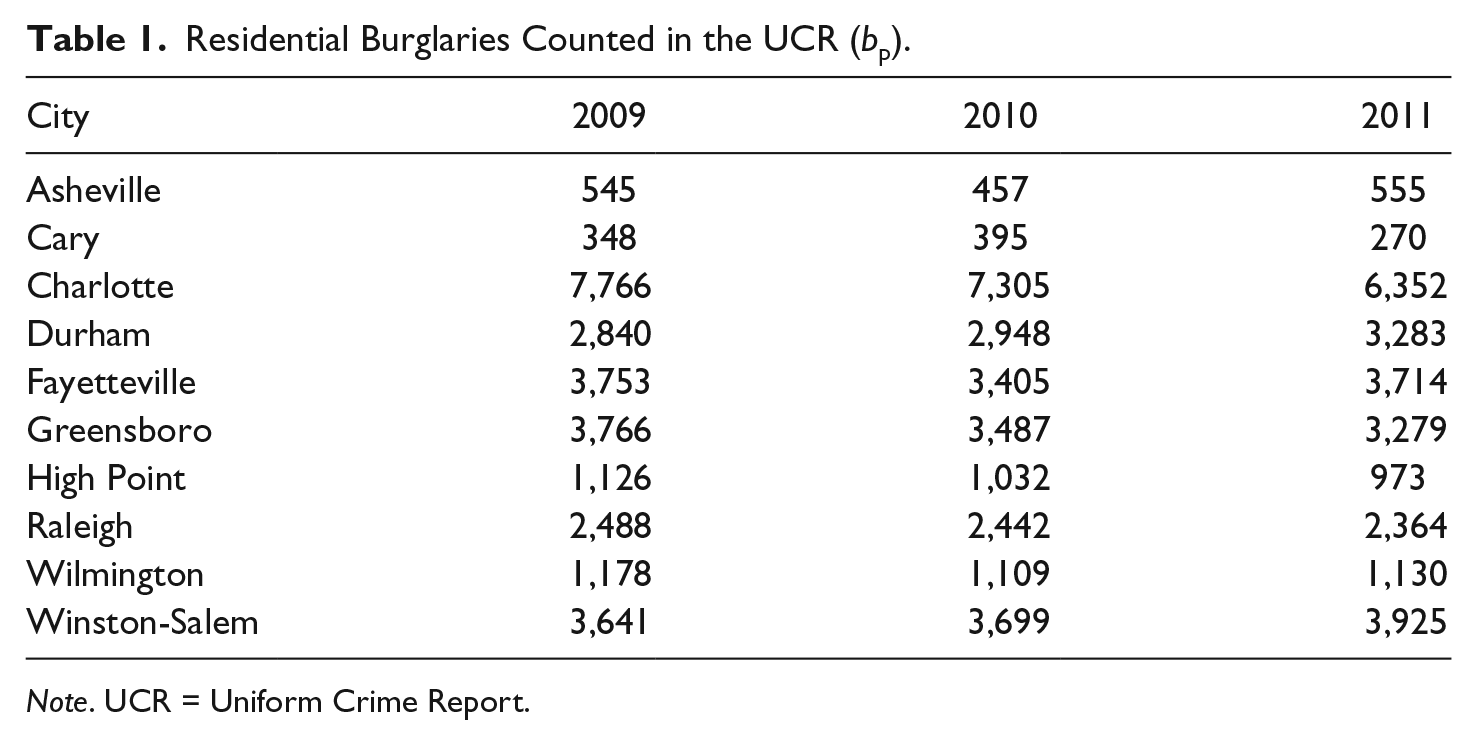
Note. UCR = Uniform Crime Report.

We formally attend to three ambiguities that arise when these burglary numbers are presented as the actual number of burglaries committed (and the derivative burglary rate per 100,000 population) in each jurisdiction: (a) the “Hierarchy Rule” for burglaries, (b) the population estimate used in estimating the burglary rate, and (c) variation in the probability that a residential burglary victim reports the incident to the police.

The first issue we encounter in interpreting the burglary numbers in Table 1 is the UCR’s Hierarchy Rule (Addington, 2006; Groves & Cork, 2008, pp. 173-175). The Hierarchy Rule mandates that any residential burglary reported to the police which co-occurs with an offense that ranks higher in the UCR hierarchy (aggravated assault, robbery, rape, or murder/non-negligent manslaughter) will not be counted as a residential burglary in the police statistics. Because of the Hierarchy Rule, we know the number of residential burglaries reported by the police to the UCR program, b_p, will generally be an undercount of the number of residential burglaries actually known to the police, which we denote as b_k. To estimate b_k, we need an estimate of the following fraction:

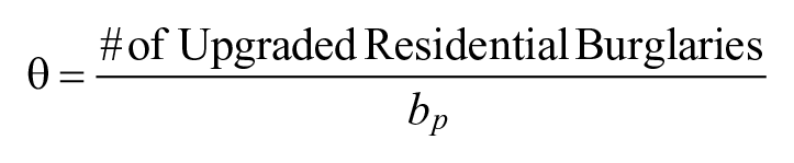
θ = \frac{# o f Upgraded Residential Burglaries}{b_{p}}

so that 1 + θ provides us with an upward adjustment to the police-reported counts to get an estimate of the number of burglaries known to the police:

b_{k} = b_{p} \times (1 + θ)

Rantala (2000, p. 7) measured crime classifications ignoring the Hierarchy Rule from the National Incident Based Reporting System (NIBRS) compared with crime classifications on the same criminal events using the traditional UCR approach. This analysis was based on a detailed study of crime reports submitted by police departments covering 1,131 jurisdictions throughout the United States in the year 1996. According to the report, the participating police agencies reported 105,852 incidents of burglary (including both residential and commercial burglary) in the NIBRS. The number of burglaries that would have been counted if the UCR’s Hierarchy Rule had been applied instead was 105,305—which implies that the shrinkage in UCR-counted burglaries due to the Hierarchy Rule (105,852-105,305 = 547) is on the order of

θ = \frac{547}{105, 305} = 0.005

An alternative analysis based on NIBRS data from 2001 compiled by Addington (2006, p. 239) suggests that θ attains an upper bound of 0.01. We therefore assume that θ could be anywhere in the interval [0.005, 0.01]. If our assumptions on the location and width of the θ interval are correct, the lower bound on b _k will be

LB (b_{k}) = b_{p} \times [1 + LB (θ)]

whereas the upper bound on b _k is

UB (b_{k}) = b_{p} \times [1 + UB (θ)]

These bounds show that the number of burglaries that appear in the police statistics slightly underestimate the number of burglaries actually known to the police. Table 2 presents the results of estimating bounds on b_k in the 10 North Carolina cities. In each of the cities in our study, estimating b_k based on θ and b_p yielded only small increases in the estimated number of residential burglaries. While the practical effect of this adjustment is small, we include it here in case new information ever appears showing that our estimate of θ is too low.

Table 2.

Residential Burglaries Known to Police (b_k).

City	2009		2010		2011
City	LB(b_k)	UB(b_k)	LB(b_k)	UB(b_k)	LB(b_k)	UB(b_k)
Asheville	548	550	459	462	558	561
Cary	350	351	397	399	271	273
Charlotte	7,805	7,844	7,342	7,378	6,384	6,416
Durham	2,854	2,868	2,999	3,014	3,299	3,316
Fayetteville	3,772	3,791	3,422	3,439	3,733	3,751
Greensboro	3,785	3,804	3,504	3,522	3,295	3,312
High Point	1,132	1,137	1,037	1,042	978	983
Raleigh	2,500	2,513	2,454	2,466	2,376	2,388
Wilmington	1,184	1,190	1,115	1,120	1,136	1,141
Winston-Salem	3,659	3,677	3,717	3,736	3,945	3,964

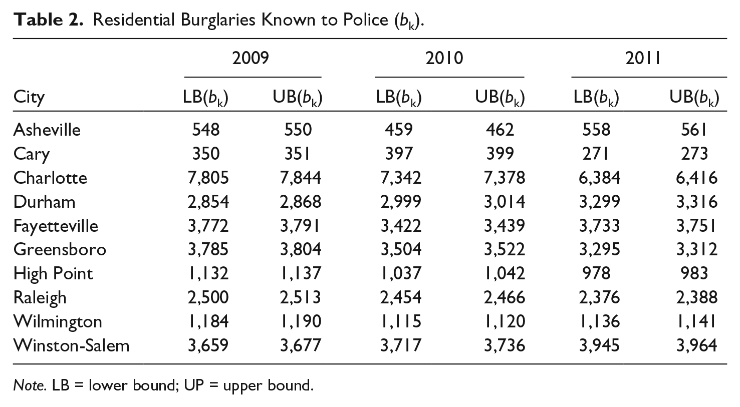
Note. LB = lower bound; UP = upper bound.

Reporting Crimes to the Police

The NCVS (and its predecessor, the NCS) is a nationally representative rotating panel household survey that has been continuously conducted by the Bureau of Justice Statistics (BJS) and the U.S. Census Bureau since 1973. Households selected to participate in the survey remain in the sample for a 3.5 year period with interviews scheduled every 6 months for each household (although approximately one sixth of the households in the survey are interviewed each month of the year). For personal victimizations, the NCVS interviewer attempts to collect data on incidents from each member of the household who is at least 12 years old. For property victimizations (including residential burglary), a designated person in the household answers all of the survey questions on behalf of the household.

There is a large literature on the similarities and differences in crime trends measured by the UCR and the NCVS (Groves & Cork, 2008; Lynch & Addington, 2006) and ways in which the UCR and the NCVS can be adjusted to better track each other (Groves & Cork, 2008, p. 74; Rand & Rennison, 2002, pp. 50-51). What is unclear is how closely these trends track each other at local levels. As the NCVS can only be deployed for these types of comparisons in special cases and at specific times (Groves & Cork, 2008, pp. 73-74; Lauritsen & Schaum, 2005), there is no general way to answer this question—it is an intrinsic source of uncertainty in our understanding of U.S. crime patterns.

In addition to asking survey respondents about victimization experiences, the NCVS interviewers ask those who experienced victimizations whether those incidents were reported to the police (Baumer & Lauritsen, 2010; Maltz, 1975). The police reporting rates stratified by crime type are a standard table presented in NCVS reports going back to the original administrations of the NCS in 1973. In the early years of the NCS, the reporting rates for residential burglaries were usually estimated to be in the range of 45% to 50%. In recent years, however, the reporting rates have mostly been in the range of 50% to 59%. Generally speaking, then, reporting rates seem to have been trending upward over time. But even as recently as 2006, the reporting rate fell below 50% and in the most recent year of data, the reporting rate was estimated to be 52%. Table 3 presents the residential burglary reporting rates, estimated standard errors of those rates, and 95% confidence limits for the 2009-2011 period of our study.

Table 3.

NCVS Burglary Reporting Rates (2009-2011).

Year	RR	SE[RR]	95% CL
Year	RR	SE[RR]	Lower	Upper
2009	57.3	1.7	54.0	60.6
2010	58.8	1.9	55.1	62.5
2011	52.0	1.8	48.5	55.5

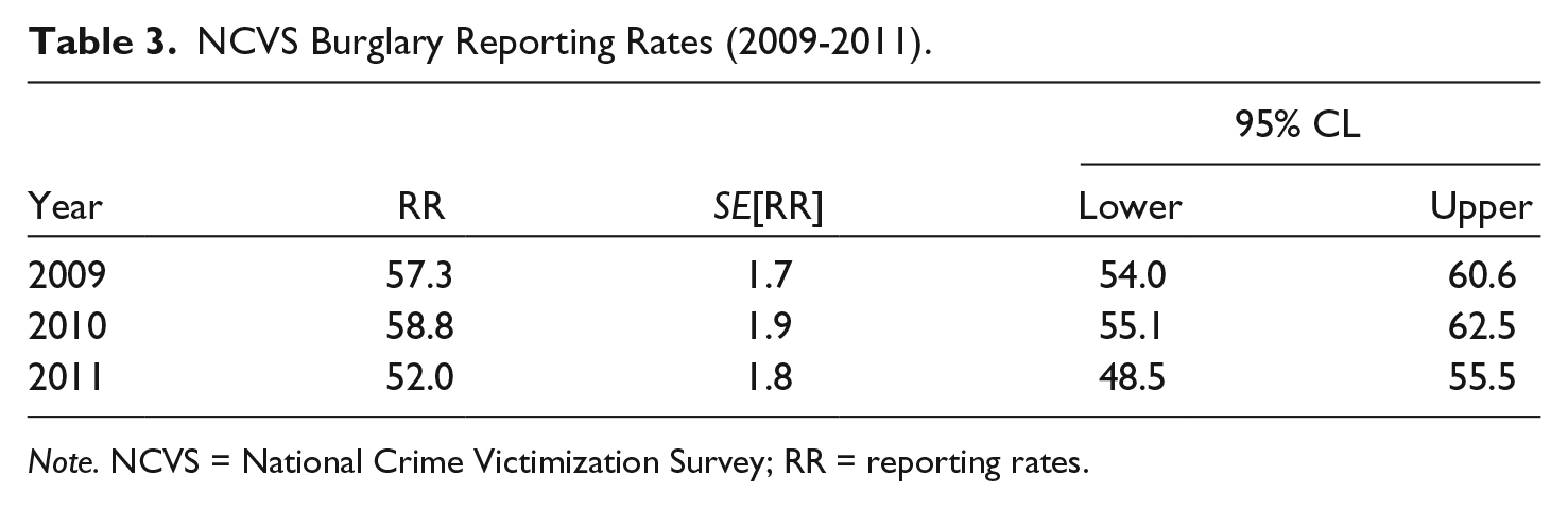
Note. NCVS = National Crime Victimization Survey; RR = reporting rates.

The reporting rate is an approximation to a critical parameter for our study—the probability that a residential burglary victim reports that victimization to the police—which we denote as p_r. For the 3 years we study closely in this article, we ignore the small problem of respondents who either did not know or did not say whether a burglary victimization was reported to the police. We assume that each city’s p_r lies within the 95% confidence interval of the national percentage of residential burglaries reported to the police in each of the 3 years, 2009-2011.

Bounding the Number of Burglaries

When researchers, police chiefs, newspaper reporters, and booksellers report overtime changes and area differences in crimes known to the police as actual crime levels, they are making the strong assumption that the probability of a crime victim reporting a victimization to the police is constant either over time or space (or perhaps both). Let us return briefly to the Charlotte Observer example cited earlier. That article reported that “the number of crimes dropped by 7.1% last year.” The only way this statement could be correct is if the reporting probability, p_r, was exactly the same from one year to the next. Since the reporting rates in Charlotte for the range of different crimes included in the Observer’s article are not well understood, there is no justification for the certitude that p_r stayed exactly the same from one year to the next. Furthermore, when researchers estimate difference-in-difference regression models or pooled cross-sectional time-series models to study the effects of this or that intervention, social, or economic trend on crime patterns, the complexity of the comparisons and ambiguities in identification propagate and the analytical difficulties remain.

We think it is preferable to develop a plausible range of values for p_r for those crimes. The range should have two key features: (a) it includes the true value of p_r and (b) it expresses the uncertainty we have about the true value of p_r. Our approach assumes that the reporting rate for each individual city lies within the 95% confidence interval of the reporting rate estimated by the NCVS in each year. A useful consequence of our approach is that it will not be possible to express the incidence of residential burglary in terms of a single number. Instead, we adopt the perspective of Manski (1995, 2003) and argue that a range of estimates based on weaker assumptions are preferable to fragile point estimates based on stronger assumptions. Even if some would take issue with the precise boundaries of our interval, we still believe it to be far more credible than a constant p_r assumption across cities or over time within the same city. And a key feature of our approach is that it is easy to use the information we present to calculate estimates based on different boundaries if there are good reasons for doing so.

We now turn to the task of estimating the actual number of residential burglaries in the 10 North Carolina cities in 2009-2011. We refer to this estimand as b_a where the subscript a means actual. What we have obtained so far are bounds on b_k which is the number of residential burglaries known to the police, allowing for uncertainty due to the UCR Hierarchy Rule. So, we need a way to move from the bounds on b_k to bounds on b_a. In a world where p_r and b_k are known with certainty, we would estimate b_a = b_k / p_r as discussed in Eck and Riccio (1979, p. 298). For example, if a community’s police department recorded b_k = 1,000 residential burglaries in 2009 and the probability that a residential burglary victim reports the incident to the police is 0.573 (the 2009 NCVS-estimated reporting rate), then it follows that the number of actual residential burglaries in 2009 would be b_a = b_k / p_r = 1,000 / 0.573 = 1,745. Since neither p_r nor b_k is known with certainty, our approach is to place bounds on b_a. If we have θ ∈ [0.005, 0.01] uncertainty due to the UCR Hierarchy Rule, our best estimate of the lower bound of b_a is to divide the lower bound of b_k by the upper bound of p_r which we assume to be 0.606. This yields a lower bound on the estimated number of residential burglaries:

LB (b_{a}) = \frac{LB (b_{k})}{UB (p_{r})} = \frac{1, 005}{0.606} = 1, 658

Conversely, the upper bound estimate is attained when

UB (b_{a}) = \frac{UB (b_{k})}{LB (p_{r})} = \frac{1, 010}{0.540} = 1, 870

So, in this instance, one could adopt the certitude that p_r is exactly equal to 0.573, which would yield a point-estimated number of 1,745 residential burglaries. By contrast, our approach is to make the following argument: (a) Based on the available evidence, if we had drawn repeated NCVS samples, we infer that 95% of the samples would have produced an estimated reporting rate between 54.0% and 60.6%; (b) we do not have local-area estimates of the reporting rates for individual cities; (c) we assume that the individual cities are within sampling error of the national estimates; (d) if our boundaries on p_r include the true value of p_r and our assumptions about the Hierarchy Rule are correct, then the number of actual burglaries lies between 1,658 and 1,870; and (e) our answer is less precise than a point estimate but our statement summarizing the results is far more likely to be correct and does a better job of transmitting both what we know and what we don’t know to our audience.

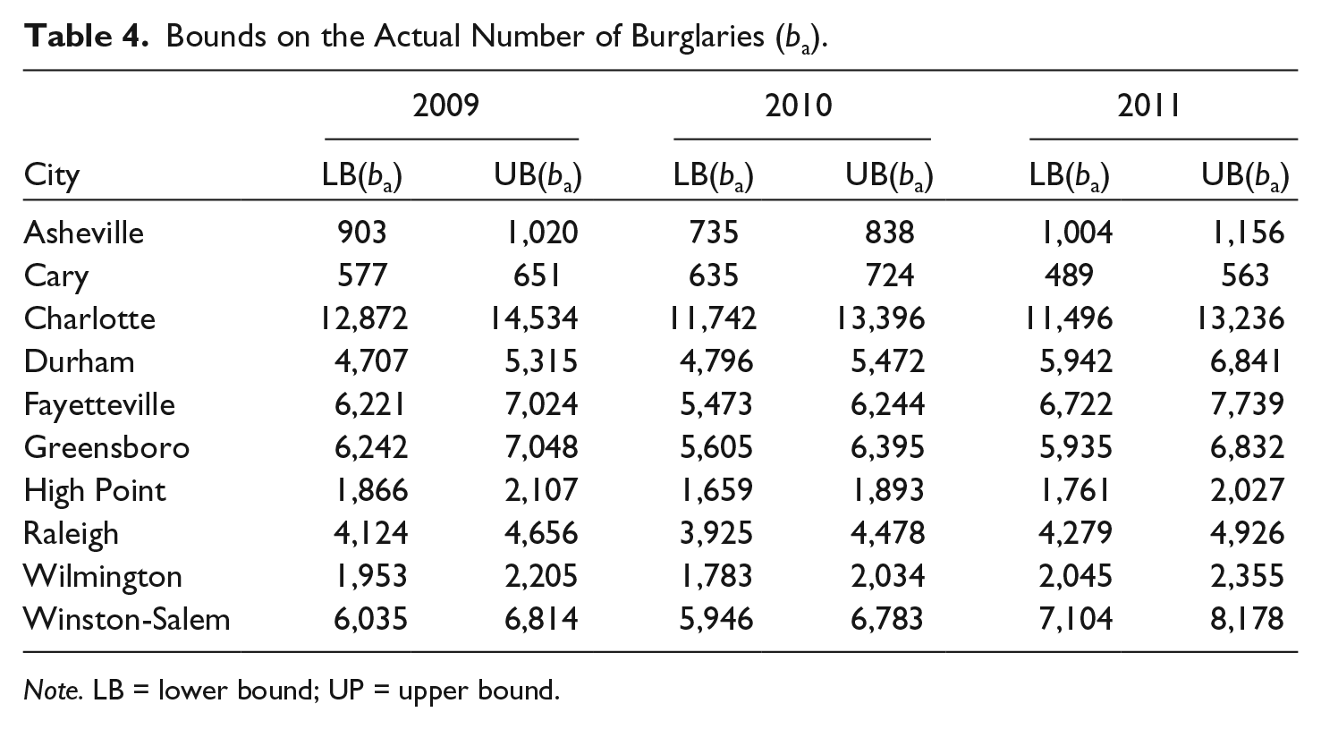
Applying this logic to the residential burglary data in the 10 North Carolina cities in 2009-2011, we estimate the bounds on the actual number of residential burglaries (Table 4), b_a. The results in Table 4 highlight some key features of our approach. Let’s consider Charlotte as an example. From Table 1, in 2010, we see that the Charlotte-Mecklenburg Police Department reported 7,305 residential burglaries while that number dropped to 6,352 burglaries in 2011 (a 13% year-over-year decline). Yet Table 4 shows that the actual number of residential burglaries in Charlotte in 2010 was between 11,742 and 13,396, whereas in 2011 it was between 11,496 and 13,221. Based on this evidence, it is not possible to definitively say whether the number of residential burglaries stayed the same, increased, or decreased from 2010 to 2011. A critical source of ambiguity in this comparison is that the 95% confidence limits for the reporting rate in 2010 and 2011 are [0.551, 0.625] and [0.485, 0.555], respectively. So, it is not possible to tell whether the decline in Charlotte burglaries reported by the police is due to real changes in burglary or changes in the reporting rate from one year to the next (or both).

Table 4.

Bounds on the Actual Number of Burglaries (b_a).

City	2009		2010		2011
City	LB(b_a)	UB(b_a)	LB(b_a)	UB(b_a)	LB(b_a)	UB(b_a)
Asheville	903	1,020	735	838	1,004	1,156
Cary	577	651	635	724	489	563
Charlotte	12,872	14,534	11,742	13,396	11,496	13,236
Durham	4,707	5,315	4,796	5,472	5,942	6,841
Fayetteville	6,221	7,024	5,473	6,244	6,722	7,739
Greensboro	6,242	7,048	5,605	6,395	5,935	6,832
High Point	1,866	2,107	1,659	1,893	1,761	2,027
Raleigh	4,124	4,656	3,925	4,478	4,279	4,926
Wilmington	1,953	2,205	1,783	2,034	2,045	2,355
Winston-Salem	6,035	6,814	5,946	6,783	7,104	8,178

Note. LB = lower bound; UP = upper bound.

Asheville serves as a counterexample. In 2010, the Asheville Police Department reported 457 residential burglaries, whereas in 2011, the number increased to 555 (a 21.4% increase). Our analysis estimates that the actual number of residential burglaries increased from the range of [735, 838] in 2010 to the range of [1004, 1156] in 2011. This means that the sign of the change in Asheville is identified (positive) even with the uncertainty that we have allowed for the reporting rates. The bottom line of Table 4 is that sometimes relatively strong conclusions are warranted—and sometimes they are not.

Population and Household Estimates

In the UCR, burglaries are defined in terms of the number of incidents per 100,000 population. The NCVS, on the other hand, defines the burglary rate in terms of the number of incidents per 1,000 households. Regardless of which approach one adopts, it is necessary—at least as a starting point—to have reasonable estimates of the number of persons living within a police department’s jurisdiction (Gibbs & Erickson, 1976). Both the SBI’s and the FBI’s UCR programs publish these estimates. We refer to the SBI estimate as n_s whereas the FBI’s estimate is denoted as n_f.⁴ Table 5 presents a summary of the two sets of population estimates for each of the cities in each year of our study.

Table 5.

Population Estimates.

City	2009		2010		2011
City	n _s	n _f	n _s	n _f	n _s	n _f
Asheville	78,267	74,923	78,804	83,393	82,846	84,450
Cary	141,269	133,757	147,282	135,234	136,203	136,949
Charlotte	738,768	777,708	752,799	779,541	776,787	789,478
Durham	221,675	227,492	227,524	228,330	222,978	231,225
Fayetteville	205,285	173,995	205,555	200,564	206,132	203,107
Greensboro	257,581	253,191	261,519	269,666	263,279	Missing
High Point	100,648	103,675	102,216	104,371	104,788	105,695
Raleigh	367,514	406,005	373,100	403,892	395,716	409,014
Wilmington	99,485	101,438	99,911	106,476	104,422	107,826
Winston-Salem	222,574	230,978	229,338	229,617	224,566	232,529

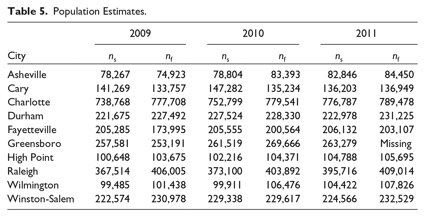
In looking at the estimates in Table 5, we are struck by how similar they are in some cases (for example, Winston-Salem and Durham in 2010) and how different they are in others (for example, Fayetteville in 2009, and Charlotte and Raleigh in 2009-2010). We do not take a position on the comparative validity of the two population estimates, but the fact that they are sometimes not close to equal adds yet another layer of uncertainty to our interpretation of the crime rate. That there would be variation in population estimates when those estimates are compiled by independent agencies is unsurprising. Summarizing the size of the population or the number of households in a particular police department’s jurisdiction in a year’s time with a single number must, on its face, be an approximation (Gibbs & Erickson, 1976). It is also interesting that textbook discussions of the crime rate often point to ambiguities in counting the number of crimes, but the ambiguities in counting the target population for any particular crime rate are a less prominent consideration (Lab et al., 2008, pp. 4-5).

A second issue is the calibration of household counts within a particular city. One could take the position of the NCVS, that residential burglary is a crime against an entire household and that residential burglaries are best expressed in terms of the risk per household rather than an individual per-person (or a scaled-up divisor such as 1,000 persons or 100,000 persons). A question that needs to be considered in any specific analysis is whether the conclusions we draw depend on the scaling unit. It is useful to consider the case where the scaling unit would not create any ambiguity. If we are able to assume that the number of persons per household is constant over time within the same city and across cities, then the choice between scaling units (persons or households) is arbitrary. On the other hand, if the number of persons per household varies over time within a jurisdiction or between jurisdictions, then our rate estimators should accommodate this variability. Table 6 relies on the data in Table 5 combined with information from the U.S. Census Bureau’s (2012) measure of the average number of persons per household (pph) in each of the 10 North Carolina cities over the period 2006-2010 to produce state and federal estimates of the number of households in each city (h_s and h_f, respectively).

Table 6.

Household Estimates.

City	pph	2009		2010		2011
City	pph	h _s	h _f	h _s	h _f	h _s	h _f
Asheville	2.13	36,745	35,175	36,997	39,152	38,895	39,648
Cary	2.68	52,712	49,909	54,956	50,460	50,822	51,100
Charlotte	2.46	300,312	316,141	306,016	316,887	315,767	320,926
Durham	2.30	96,380	98,910	98,923	98,274	96,947	100,533
Fayetteville	2.48	82,776	70,159	82,885	80,873	83,118	81,898
Greensboro	2.34	110,077	108,201	111,760	115,242	112,512	Missing
High Point	2.51	40,099	41,305	40,724	41,582	41,748	42,110
Raleigh	2.35	156,389	172,768	158,766	171,869	168,390	174,049
Wilmington	2.19	45,427	46,319	45,621	48,619	47,681	49,236
Winston-Salem	2.42	91,973	95,445	94,768	94,883	92,796	96,086

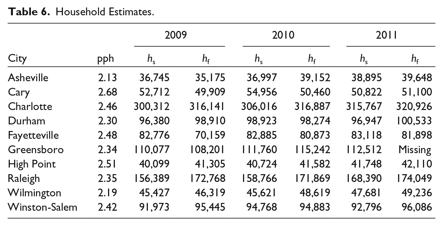
A prominent aspect of the evidence in Table 6 is that there is real variation in the number of persons per household in large North Carolina cities. On average, Asheville and Wilmington have smaller household sizes (< 2.2 persons per household), whereas Cary and High Point have the highest density households (> 2.5 persons per household). It is possible, then, that two cities could have an identical rate of residential burglary when that rate is expressed in terms of population size but have different residential burglary rates when expressed in terms of the number of households in the city.

Estimating Residential Burglary Rates

We now consider how much our inferences about residential burglary rates depend upon the issues we have considered in this article. We don’t expect much sensitivity to the uncertainty of the Hierarchy Rule since the adjustments are small. It is less clear how sensitive our results will be to uncertainty about the size of the population (including whether we scale by the number of persons or the number of households) and uncertainty about the fraction of residential burglaries reported to the police.

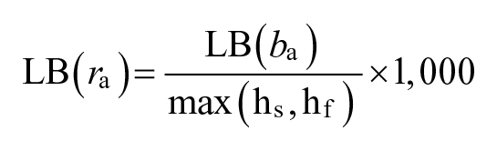
To estimate the actual rate of residential burglaries per 100,000 persons, r_a, we define its lower bound as follows:

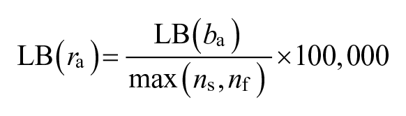
LB (r_{a}) = \frac{LB (b_{a})}{\max (n_{s}, n_{f})} \times 100, 000

whereas the upper bound is

UB (r_{a}) = \frac{UB (b_{a})}{\min (n_{s}, n_{f})} \times 100, 000

This interval estimate identifies the outer limits of what is possible in terms of the residential burglary rate per 100,000 persons assuming that n_s and n_f form the proper bounds on the size of the population, that each city’s reporting rate falls within the 95% confidence interval of the NCVS-estimated reporting rate, and that our adjustments for the FBI’s Hierarchy Rule are accurate. We combine these estimates with the standard residential burglary rates per 100,000 population based on the information from Tables 1 and 5 to produce the point and interval estimates in Figure 1.

Figure 1.

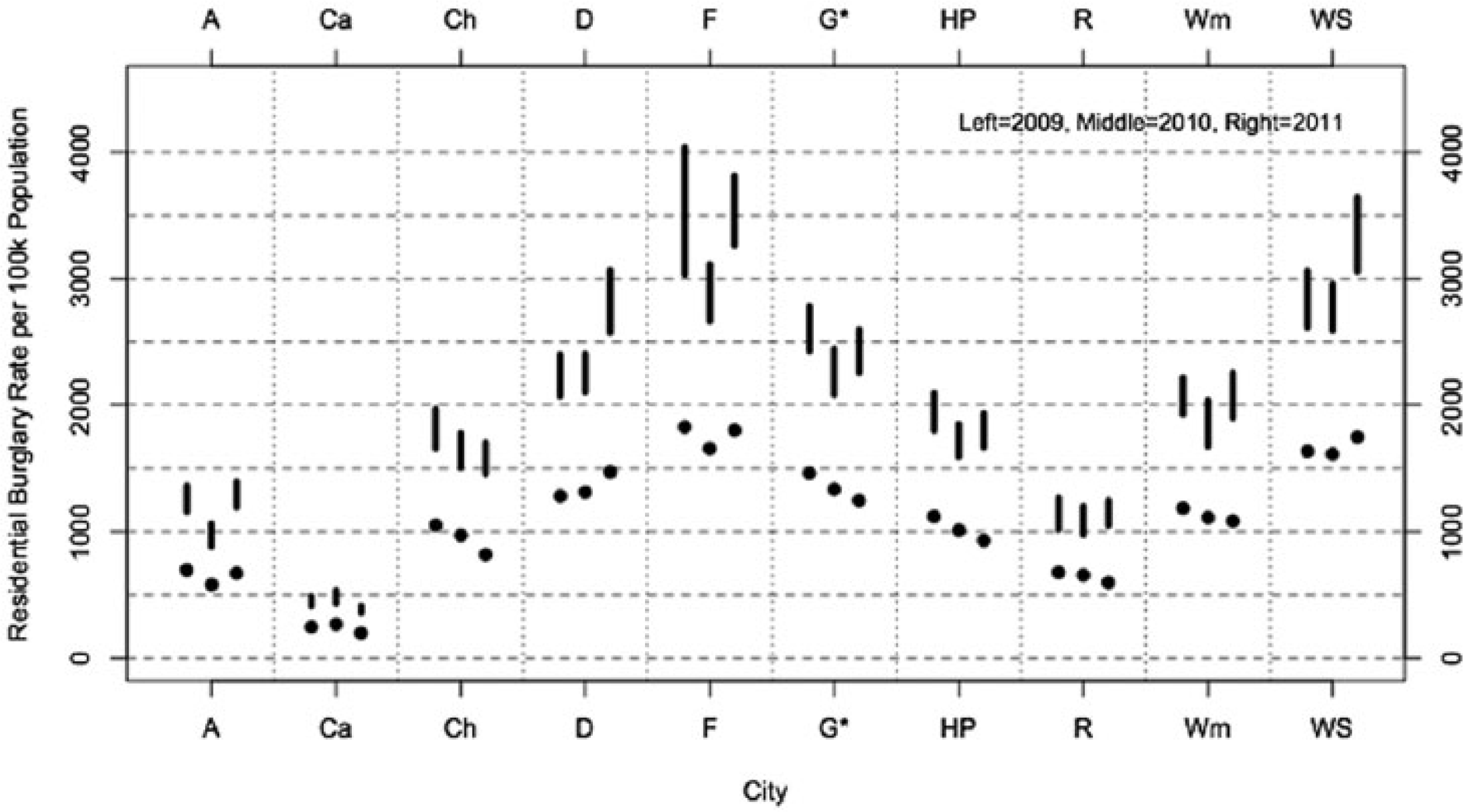
Residential burglary rate (population) estimates.

For each of the 10 cities in Figure 1, there are 2 sets of estimates: (a) the upper and lower bound (interval) estimates of the actual residential burglary rate (r_a) for 2009-2011 and (b) the “standard” (point) estimates of the residential burglary rate per 100,000 population (based on Tables 1 and 5) for 2009-2011.⁵ Comparisons between the point estimates over time within the same city implicitly assume that the reporting rate, p_r, is the same across the years whereas comparisons between point estimates of different cities implicitly assume that the reporting rate is constant between the cities being compared (at the time they are compared). Although these assumptions seem implausibly strong, they are commonly invoked for both journalistic and research purposes.

We also consider the impact of adjusting for the number of households instead of the number of people and then placing residential burglaries on a scale per 1,000 households in each city during each year (Figure 2). This analysis relies on the information presented in Tables 4 and 6. To estimate the lower bound on the residential burglary rate per 1,000 households, we obtain

LB (r_{a}) = \frac{LB (b_{a})}{\max (h_{s}, h_{f})} \times 1, 000

Figure 2.

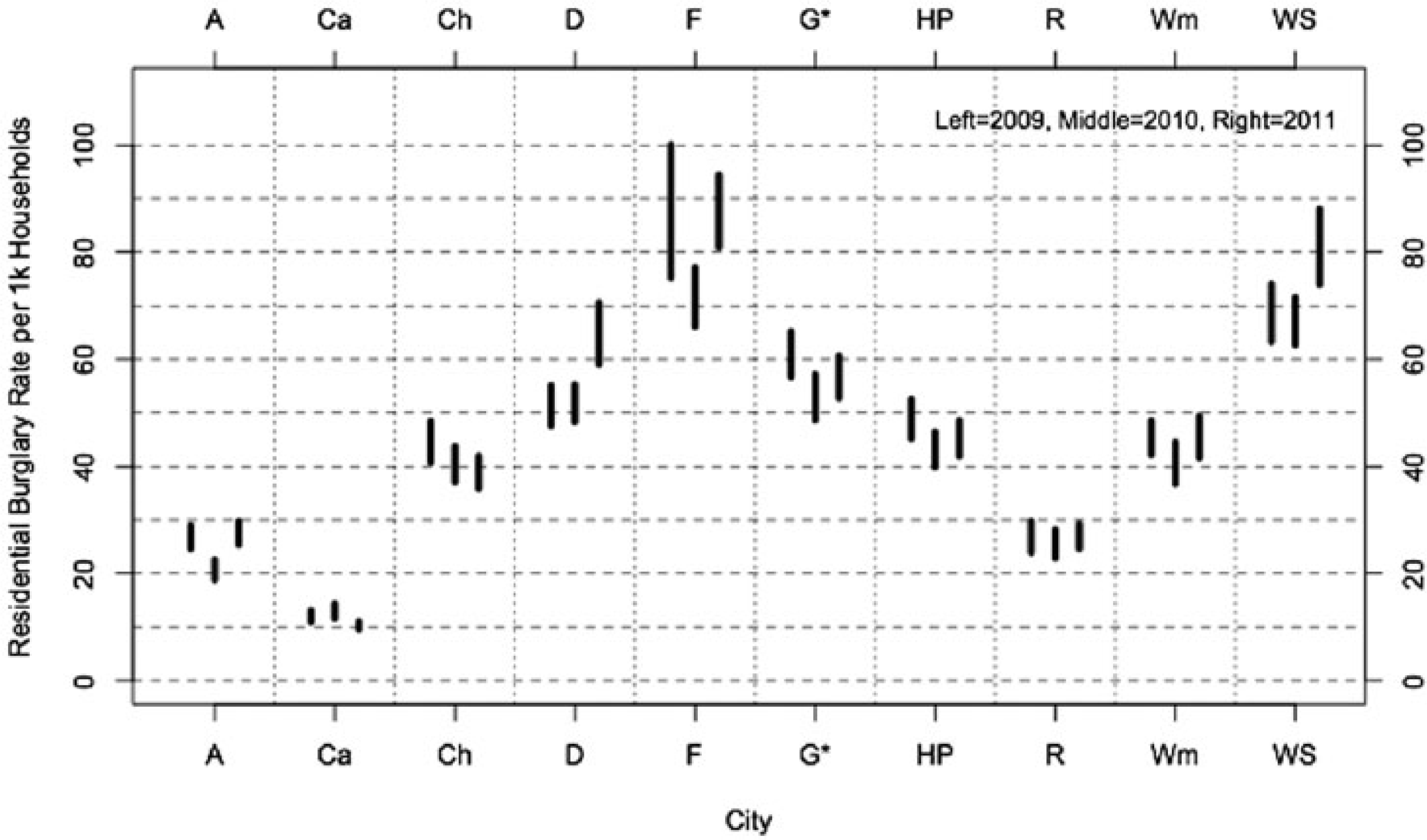
Residential burglary rate (household) estimates.

and the upper bound is given by

UB (r_{a}) = \frac{UB (b_{a})}{\min (h_{s}, h_{f})} \times 1000

Broadly speaking, the two sets of rate comparisons in Figures 1 and 2 seem to tell similar stories. From this analysis, we conclude that the major source of uncertainty in estimating residential burglary rates in these 10 North Carolina cities over the 2009-2011 time frame is the reporting rate, and to a lesser extent, the size of the population. It is worth considering a couple of example implications of our results. Suppose we set out to compare the burglary rates between Charlotte and Wilmington in 2009. Using the standard approach for comparing the two cities, we would find that Charlotte had a residential burglary rate of 1,051 per 100,000 persons, whereas Wilmington’s rate is 1,184 (nearly 13% higher). Some might use this evidence to say that Wilmington had a higher residential burglary rate than Charlotte in 2009. But upon further analysis, we find that the actual rate of residential burglaries per 100,000 population could plausibly lie in the [1656, 1967] interval in Charlotte and the [1925, 2216] interval in Wilmington. Because these intervals overlap (see Figure 1), the sign of the difference between Charlotte and Wilmington is not identified.

This lack of identifiability becomes even more prominent when we focus on household incidence of burglary. For Charlotte, the bounds on the residential burglary rate per 1,000 households in 2009 are [40.72, 48.40]; for Wilmington, the bounds are [42.16, 48.53]. This is a marked increase in the degree of overlap between the Charlotte and Wilmington interval estimates. We can attribute most of this difference to the fact that Charlotte households had an average of 2.46 persons in 2006-2010, whereas Wilmington households were smaller on average (2.19 persons) over the same time period. In short, to speak about a clear difference in these two cities is an example of unwarranted certitude. It is possible that Charlotte’s burglary rate is higher, lower, or the same as Wilmington’s. Considering plausible sources of uncertainty in the comparison, the data are simply not strong enough to tell us.

A comparison of Charlotte and Raleigh—on the other hand—leads us to a stronger set of conclusions. In 2011, for example, Charlotte’s estimated residential burglary rate per 100,000 population—based exclusively on the information in Tables 1 and 5—was 818 whereas Raleigh’s rate was 597 (a [818 − 597] / 818 × 100 ≈ 27% difference). We conclude that the difference between the burglary rates in Charlotte and Raleigh cannot be explained by the uncertainties considered in this article. The residential burglary rate interval for Charlotte in 2011 is [1456, 1704], whereas the interval for Raleigh in the same year is [1046, 1245]. As Figure 2 shows, there is a similar pattern for burglary incidence scaled by the number of households. As these intervals do not overlap, it seems credible to argue that Charlotte’s rate is higher than Raleigh’s rate in 2011.⁶

Figures 1 and 2 are also helpful for displaying the overtime change within cities. Using the standard crime rate estimator, we can see that the point estimates of Charlotte’s residential burglary rate reveal what appears to be a meaningful decline from 2009 (1,051) to 2011 (818) (a drop of about [818 − 1,051] / 1,051 × 100 ≈ 22.2%). The problem is that there is some evidence that reporting rates could have also changed a good deal over the same time period. What this means is that the burglary rate interval for Charlotte (accounting for the Hierarchy Rule, reporting rate uncertainty, and population size uncertainty) is [1655, 1967] in 2009 and [1456, 1704] in 2011. As these intervals overlap, we cannot discern whether the Charlotte burglary rate increased, decreased, or stayed the same over this time period. A counterexample is provided by Durham. In 2009, the standard burglary rate estimate was 1,281; in 2011 that rate estimate increased to 1,472—an increase of [1,472 − 1,281] / 1,281 × 100 ≈ 14.9%. Our interval estimates suggest that this increase was real; in 2009, the interval was [2069, 2398], whereas in 2011, the entire interval shifted up to [2570, 3068]. In the case of Durham, we can confidently conclude that residential burglaries increased—why that increase occurred, of course, is a different question.

Conclusions

A good deal of contemporary discussion about local crime patterns in the U.S. is marred by unwarranted certitude about the numbers and rates underlying that discussion. Criminal justice officials, journalists, and even academic criminologists count crimes known to the police while ignoring key sources of uncertainty about those numbers. Since the late 1960s and early 1970s, for example, it has been common criminological knowledge that many crimes are not reported to the police but somehow that knowledge ends up playing only a tangential role (if any role at all) in our public discourse about crime patterns at the local level, although more recent research has directly assessed the impact that citizen reporting rates have on police measures of crime (see Xie, 2014).

Part of the problem is that there has been little methodological attention to the task of expressing and transmitting uncertainty about crime patterns to policy and lay audiences (Manski, 2003, p. 21). Based on Manski’s work on bounds and partial identification, however, we think it will be useful for criminologists to begin reporting crime patterns in terms of a range of uncertainty that expresses both what is known and unknown about the numbers that are used to measure those patterns. A key feature of the methods used here is that they explicitly abandon the goal of obtaining point estimates in favor of a more realistic and reasonable goal of obtaining interval estimates. Our approach provides one path by which criminologists can begin to reasonably express both what is known and unknown with current publicly available datasets.

Another feature of our approach is that we move away from the “incredible certitude” problem described by Charles Manski (2011)—the practice of developing unqualified and unjustifiably “certain” inferences based on weak data. Criminologists are often asked by the media to comment on small year-to-year movements in police-based crime statistics. In our conversations with other criminologists, we have noted that many feel quite uncomfortable characterizing this or that movement in the crime rate. The analysis in this article illustrates why these feelings of apprehension are justified. As Eck and Riccio (1979) observed over 30 years ago, a movement of a few percentage points in the police statistics may or may not reflect real changes in crime. We think our approach to this problem is useful because it allows us to transmit our uncertainty—especially to lay audiences—in systematic ways that have not been obvious in the past.

Still, there are limitations. First and foremost, we believe our bounds on the probability that a residential burglary is reported to the police (p_r) are a reasonable starting point but improving our understanding of this interval would be constructive. This highlights an important direction for future research: Achieving disciplinary consensus on the likely bounds for crime reporting probabilities should be a high priority. One reviewer of a previous version of this manuscript criticized our reporting rate intervals as being too narrow. That reviewer found it inconceivable that the local and national estimates would exhibit any particular comparability.

Most of the data that can be used to check on this were collected in the 1970s in a series of city crime surveys conducted by the National Criminal Justice Information and Statistics Service (1974, 1975, 1976; see also Levitt, 1998) and a research report by Lauritsen and Schaum (2005). While there is not much local data to go on, it appears from the weight of this evidence that most cities have residential burglary reporting rates that are within a reasonably proximate range of the national estimates of their time. The reviewer’s comment nonetheless highlights the need for greater understanding of how closely local reporting rates track what is observed nationally (Xie, 2014). And—if the reviewer turns out to be correct—then the burglary rate intervals estimated in our work will be too narrow, a result which amplifies rather than diminishes our arguments.

We have considered several examples where point estimates based on conventional methods prove to be highly misleading. Using those methods one would draw the conclusion that one city had a higher rate than another city or that a city’s rate changed in a meaningful way from one year compared with another. Our analysis shows that in some of these comparisons, a plausible rival hypothesis cannot be excluded: It is possible that the burglary rates are the same while only the reporting rate differs. Since the reporting rate, p_r, is not identified—we can only make assumptions about its value—the data cannot be used to resolve this ambiguity. Only information that reduces our uncertainty about the rate at which residential burglaries are reported to the police in the two cities will resolve it.

The good news is that the development of this kind of information is feasible. The National Research Council along with the BJS has recently considered a range of possibilities for improving on the small-area estimation capabilities of the NCVS (Bureau of Justice Statistics, 2010; Groves & Cork, 2008; Pepper & Petrie, 2003). Most of the attention has focused on small-area estimation of victimization rates, but further refinement of reporting rate estimates should also be a priority. This is not a new idea—focusing on the limitations of the FBI data, Eck and Riccio (1979) emphasized the possibilities of this approach decades ago—yet combining this emphasis with a focus on interval estimation of crime rates may prove to be a viable way forward. A key benefit of this kind of information would be a substantial reduction of the uncertainty that is evident in our Figures 1 and 2.

It is noteworthy that we are able to make useful statements about residential burglary rates for North Carolina cities because the state reporting program clearly identifies residential burglaries known to the police. This is not done in the FBI’s UCR which presents counts of all burglaries - both residential and commercial - known to the police in a single number. And we encounter difficulty using the FBI’s burglary numbers since the NCVS only measures reporting behaviors for residential burglaries. Expansion of our approach to other crimes will require careful consideration of how the crimes described in the UCR relate to the victimization incidents counted in the NCVS. There is a well-developed literature on this topic (see, for example, Blumstein et al., 1991, 1992; Lynch & Addington, 2006) but there will be some difficulties in ensuring that the reporting probability gleaned from the NCVS maps onto UCR crime categories in a meaningful way. In our view, the field will be well served by taking on these challenges.

We encountered a few other ambiguities in addition to the reporting probability, namely, uncertainty due to the UCR’s Hierarchy Rule, the size of the population, and the question of whether to scale by the number of households or by the number of persons (Gibbs & Erickson, 1976). It is surprising how large some of the differences in population estimates were and this uncertainty should be considered in more detail. We verified that each of the jurisdictions we studied participated in the state UCR Program each month of each year during the 2009-2011 calendar years (but Greensboro did not participate in the federal program in 2011); still we clearly have no way to verify the accuracy of the numbers reported by the police departments (Westat, 2010, pp. VII-VIII). This issue is always a threat to analyses that rely on police-based crime statistics and our study is no exception.

An anonymous reviewer of a previous version of this article also highlighted the need to consider the actual population at risk for other crimes besides burglary. We quite agree. For example, in cities where there are many tourists or many people who commute from neighboring communities, the population at risk for victimization for crimes like robberies and assaults is, in general, a very different number of people than the number of persons who live in the city. In general, the number of people who live in the city is smaller and, as the reviewer suggests, this can dramatically inflate the crime rate. It is simply not reasonable to compare personal robbery rates in cities where the population count based on the actual “feet on the street” is significantly larger than the number of people who actually reside in the city. Yet these comparisons are routinely conducted with no adjustment for this kind of variability. Although this issue is less of a problem for the residential burglaries considered in this article (as those are crimes against households), it is a major obstacle to clear inference about between-places variability in other kinds of crimes.

In our view, it will be useful for criminologists to (a) be aware of the kinds of uncertainties discussed in this article; (b) develop better information about uncertain parameters—such as the probability of victimizations being reported to the police at the local level; (c) create analytic methods that will formally incorporate and transmit key sources of uncertainty in the measurement of crime rates; and (d) explore ways of conducting sensitivity analysis to assess the fragility of our results. A fifth priority should be a program of research to consider how identification problems such as those discussed in this article can be addressed within the framework of statistical models commonly used to estimate effects of social and economic changes on crime rates. Logically, there is no difference between a comparison of burglary rates in Charlotte and Raleigh from 2009 to 2010 and the kinds of panel regression, difference-in-difference, and pooled-cross-sectional time-series estimators commonly used to identify causal relationships in crime data. All of the uncertainties discussed here are present in space-and-time crime regressions commonly estimated by criminologists. Yet the issues discussed in this article loom as major sources of uncertainty for these models. We view our approach as an initial, constructive, and necessary step in the direction of a more balanced and informative use of aggregate crime statistics.

Footnotes

Declaration of Conflicting Interests

The author(s) declared no potential conflicts of interest with respect to the research, authorship, and/or publication of this article.

Funding

The author(s) received no financial support for the research, authorship, and/or publication of this article.

Notes

Author Biographies

Robert Brame is a professor in the Department of Criminology and Criminal Justice at the University of South Carolina. His research interests include criminal recidivism, the prevalence of criminal justice system involvement, and crime measurement.

Michael G. Turner is a professor in the Department of Criminal Justice and Criminology at the Univerisity of North Carolina at Charlotte. His research interests include victimization, juvenile delinquency, and testing criminological theories.

Raymond Paternoster is a professor in the Department of Criminology at the University of Maryland. His research interests include criminal desistance, offender decision making, and issues related to capital punishment.

References

Addington

L. A.

(2006). Using NIBRS to study methodological sources of divergence between the UCR and NCVS. In Lynch

J. P.

Addington

L. A.

(Eds.), Understanding crime statistics: Revisiting the divergence of the NCVS and UCR (pp. 225-250). New York, NY: Cambridge University Press.

American Society of Criminology. (2007). Official policy position of the Executive Board of the American Society of Criminology with respect to the use of Uniform Crime Reports data. Columbus, OH: Author.

Anderson

(1999). Code of the street: Decency, violence, and the moral life of the inner city. New York, NY: W.W. Norton.

Baumer

E. P.

Lauritsen

J. L.

(2010). Reporting crime to the police 1973-2005: A multivariate analysis of long-term trends in the National Crime Survey (NCS) and National Crime Victimization Survey (NCVS). Criminology, 48, 131-185.

Bialik

(2010, December 4). In crime lists, nuance is a victim. Wall Street Journal. Retrieved from http://www.wsj.com/articles/SB10001424052748703989004575652773618020254

Biderman

A. D.

Reiss

A. J.

Jr. (1967). On exploring the “dark figure” of crime. Annals of the American Academy of Political and Social Science, 374, 733-748.

Blumstein

Cohen

Rosenfeld

(1991). Trend and deviation in crime rates: A comparison of UCR and NCS data for burglary and robbery. Criminology, 29, 237-263.

Blumstein

Cohen

Rosenfeld

(1992). The UCR-NCS relationship revisited: A reply to Menard. Criminology, 30, 115-124.

Blumstein

Rosenfeld

(2008). Factors contributing to U.S. crime trends. In Goldberger

A. S.

Rosenfeld

(Eds.), Understanding crime trends (pp. 13-44). Washington, DC: National Academy Press.

10.

Brier

S. S.

Fienberg

S. E.

(1980). Recent economic modeling of crime and punishment. Evaluation Review, 4, 147-191.

11.

Bureau of Justice Statistics. (2010). Questions and answers from the 4/27/10 NCVS redesign session on sub-national estimates. Washington, DC: U.S. Department of Justice.

12.

Carbon

S. B.

(2012). Statement before the committee on the judiciary of the United States House of Representatives of February 16, 2012. Washington, DC: U.S. Department of Justice.

13.

Eck

J. E.

Riccio

L. J.

(1979). Relationship between reported crime rates and victimization survey results: An empirical and analytical study. Journal of Criminal Justice, 7, 293-308.

14.

Fagan

Tyler

T. R.

(2005). Legal socialization of children and adolescents. Social Justice Research, 18, 217-242.

15.

Federal Bureau of Investigation. (2009). The nation’s two crime measures. Washington, DC: U.S. Department of Justice.

16.

Gibbs

J. P.

Erickson

M. L.

(1976). Crime rates of American cities in an ecological context. American Journal of Sociology, 82, 605-620.

17.

Groves

R. M.

Cork

D. L.

(Eds.). (2008). Surveying victims: Options for conducting the National Crime Victimization Survey. Washington, DC: National Academy Press.

18.

James

Council

L. R.

(2008). How crime in the United States is measured. Washington, DC: Congressional Research Service.

19.

Kirk

D. S.

Matsuda

(2011). Legal cynicism, collective efficacy, and the ecology of arrest. Criminology, 49, 443-472.

20.

Kirk

D. S.

Papachristos

A. V.

(2011). Cultural mechanisms and the persistence of neighborhood violence. American Journal of Sociology, 116, 1190-1233.

21.

Lab

S. P.

Williams

M. R.

Holcomb

J. E.

Burek

M. W.

King

W. R.

Buerger

M. E.

(2008). Criminal justice: The essentials. New York, NY: Oxford University Press.

22.

Lauritsen

J. L.

Schaum

R. J.

(2005). Crime and victimization in the three largest metropolitan areas, 1980-1998. Washington, DC: U.S. Department of Justice.

23.

Levitt

S. D.

(1998). The relationship between crime reporting and police: Implications for the use of Uniform Crime Reports. Journal of Quantitative Criminology, 14, 61-81.

24.

Lohr

Prasad

N. G. N.

(2003). Small area estimation with auxiliary survey data. Canadian Journal of Statistics, 31, 383-396.

25.

Lynch

J. P.

Addington

L. A.

(Eds.). (2006). Understanding crime statistics: Revisiting the divergence of the NCVS and UCR. New York, NY: Cambridge University Press.

26.

Lyttle

(2012, January 18). CMPD says crime drops 7.1% in 2011. The Charlotte Observer. Retrieved from http://www.newsrt.us/news/cmpd-says-crime-drops-7-1-in-2011-351956.html

27.

Maltz

M. D.

(1975). Crime statistics: A mathematical perspective. Journal of Criminal Justice, 3, 177-194.

28.

Maltz

M. D.

(1999). Bridging gaps in police crime data. Washington, DC: U.S. Department of Justice.

29.

Manski

C. F.

(1995). Identification problems in the social sciences. Cambridge, MA: Harvard University Press.

30.

Manski

C. F.

(2003). Partial identification of probability distributions. New York, NY: Springer-Verlag.

31.

Manski

C. F.

(2011). Policy analysis with incredible certitude. The Economic Journal, 121, F261-F289.

32.

Merton

R. K.

(1968). Social theory and social structure. New York, NY: Free Press.

33.

National Criminal Justice Information and Statistics Service. (1974). Criminal victimization surveys in the nation’s five largest cities. Washington, DC: U.S. Department of Justice.

34.

National Criminal Justice Information and Statistics Service. (1975). Criminal victimization surveys in 13 American cities. Washington, DC: U.S. Department of Justice.

35.

National Criminal Justice Information and Statistics Service. (1976). Criminal victimization surveys in 8 American cities. Washington, DC: U.S. Department of Justice.

36.

Nelson

J. F.

(1979). Implications for the ecological study of crime: A research note. In Parsonage

W. H.

(Ed.), Perspectives on victimology (pp. 21-28). Beverly Hills, CA: SAGE.

37.

Papachristos

A. V.

Meares

Fagan

(2011). Why do offenders obey the law? The influence of legitimacy and social networks on active gun offenders. (Unpublished paper). Yale University, New Haven, CT.

38.

Paternoster

Brame

Bachman

Sherman

L. W.

(1997). Do fair procedures matter? The effect of procedural justice on spouse assault. Law & Society Review, 31, 163-204.

39.

Pepper

J. V.

(2001). How do response problems affect survey measurement of trends in drug use? In Informing America’s policy on illegal drugs: What we don’t know keeps hurting us (pp. 321-347). Washington, DC: National Academy Press.

40.

Pepper

J. V.

Petrie

C. V.

(Eds.). (2003). Measurement problems in criminal justice research: Workshop summary. Washington, DC: National Academy Press.

41.

Raghunathan

T. E.

Xie

Schenker

Parsons

V. L.

Davis

W. W.

Dodd

K. W.

Feuer

E. J.

(2007). Combining information from two surveys to estimate county-level prevalence rates of cancer risk factors and screening. Journal of the American Statistical Association, 102, 474-486.

42.

Rand

M. R.

Rennison

C. M.

(2002). True crime stories? Accounting for differences in our national crime indicators. Chance, 15, 47-51.

43.

Rantala

R. R.

(2000). Effect of NIBRS on crime statistics. Washington, DC: U.S. Department of Justice.

44.

Reisig

M. D.

Wolfe

S. E.

Kristy

(2011). Legal cynicism, legitimacy, and criminal offending. Criminal Justice and Behavior, 38, 1265-1279.

45.

Rosenfeld

Lauritsen

J. L.

(2008). The most dangerous crime rankings. Contexts, 7, 66-67.

46.

Sampson

R. J.

Bartusch

D. J.

(1998). Legal cynicism and (subcultural?) Tolerance of deviance: The neighborhood context of racial differences. Law and Society Review, 32, 777-804.

47.

Skogan

W. G.

(1974). The validity of official crime statistics: An empirical investigation. Social Science Quarterly, 55, 25-38.

48.

Slocum

L. A.

Taylor

T. J.

Brick

B. T.

Esbensen

F.-A.

(2010). Neighborhood structural characteristics, individual-level attitudes, and youths crime reporting intentions. Criminology, 48, 1063-1100.

49.

State Bureau of Investigation (North Carolina). (2012). Crime in North Carolina (2009-11). Raleigh: North Carolina Department of Justice.

50.

Sunshine

Tyler

T. R.

(2003). The role of procedural justice and legitimacy in shaping public support for policing. Law & Society Review, 37, 513-547.

51.

Swidler

(1986). Culture in action: Symbols and strategies. American Sociological Review, 51, 273-286.

52.

Truman

J. L.

(2011). Criminal victimization 2010. Washington, DC: U.S. Department of Justice.

53.

Truman

J. L.

Planty

(2012). Criminal victimization 2011. Washington, DC: U.S. Department of Justice.

54.

Tyler

T. R.

(2006). Why people obey the law. New Haven, CT: Yale University Press.

55.

Tyler

T. R.

Fagan

(2008). Legitimacy and cooperation: Why do people help the police fight crime in their communities? Ohio State Journal of Criminal Law, 6, 231-274.

56.

U.S. Census Bureau. (2012). State and County QuickFacts. Washington, DC: U.S. Department of Commerce.

57.

Wainer

(1986). The SAT as a social indicator: A pretty bad idea. In Wainer

(Ed.), Drawing inferences from self-selected samples (pp. 7-21). New York, NY: Springer-Verlag.

58.

Westat. (2010). NCVS task 4 report: Summary of options relating to local area estimation. Rockville, MD: Author.

59.

Xie

(2014). Area differences and time trends in crime reporting: Comparing New York with other metropolitan areas. Justice Quarterly, 31, 43-73.