Employment Risk,Returns,and Entrepreneurship

Abstract

Comparing local employment portfolios against entrepreneurship, this research finds that local wage and salary job market prospects shape incentives for potential entrepreneurs. Entrepreneurship may thus be more attractive in areas featuring high employment risk and/or low returns. This research contributes to the existing regional employment portfolio literature by using more disaggregated data at both the county and the commuting zone levels. Commuting zones in particular represent a broader spectrum of labor market agglomerations across both rural and urban areas to provide the most stringent and revealing tests of the interrelationship between local employment portfolios and the choice to pursue entrepreneurship. The authors find a U-shaped risk/return trade-off using employment variance and growth, consistent with the literature. They test their hypothesis with a model of regional entrepreneurship, incorporating the employment portfolio variables. This is the first known study to explore the hypothesized relationship between wage and salary employment portfolios and entrepreneurship, effectively synthesizing two previously disparate literatures.

Keywords

entrepreneurship employment portfolio self-employment employment risk establishment births

Introduction

Research examining the determinants of entrepreneurship often fails to consider the behavior of local labor markets. Entrepreneurship may be more attractive in areas featuring high employment risk and/or low returns. Better understanding of how labor market risks and returns incent nascent entrepreneurs will help advance entrepreneurship research and improve the implementation of effective economic development policies and programs. This research finds that, when comparing employment portfolios against regional entrepreneurship, measured empirically with self-employment and establishment birth rates, local wage and salary job market prospects indeed shape incentives for potential entrepreneurs.

This research makes contributions to both the employment portfolio and entrepreneurship literature, as they relate to local labor market research and economic development. The research is the first known to connect regional employment portfolio theory with entrepreneurship, particularly in terms of the incentive to pursue self-employment given the risk/return patterns of local wage and salary positions. Second, this research represents the first consistently successful application of portfolio theory to labor markets; we consider more localized data than states and metros (commuting zones [CZs] as well as counties) to evaluate the underlying relationships in the most revealing geographic detail that still represents cohesive labor markets. In particular, CZ analysis has the advantage of broadening the context of inquiry to both metropolitan and nonmetropolitan areas through a consistent taxonomy of labor market agglomerations defined by commuting sheds.

In the section Portfolio Theory and Regional Applications, we set up the trade-off between paid employment and self-employment in counties and CZs, drawing on the employment portfolio theory literature, which differs from, but has roots in, financial portfolio analysis. Seminal literature describes a risk/return tradeoff using employment variance and growth and suggests that the trade-off often features an underappreciated U shape (Chandra, 2002; Lande, 1994; Spelman, 2006). We find evidence of this U shape for smaller areal units.

The section Entrepreneurship Incentives explores the likely supply-side influence of wage and salary employment portfolios on engagement in entrepreneurial activity by empirically testing whether employment portfolios affect the next period’s self-employment and establishment birth rates. We test our hypothesis by incorporating the employment portfolio variables into a model of regional entrepreneurship. Findings suggest that the employment portfolio affects entrepreneurship. By better understanding the determinants of entrepreneurship and how job prospects affect entrepreneurship, policy makers can better foster entrepreneurship. The Conclusions section summarizes the findings and contributions and concludes with policy recommendations.

Portfolio Theory and Regional Applications

Regional Employment Applications of Portfolio Theory

Regional employment portfolio theory, clearly established in the regional science literature, is the portfolio theoretic approach to economic growth and stability. To this point, the focus of regional employment portfolio analysis has been on finding the optimal mix of industries in a region (Barry & Kearney, 2006; Barth, Kraft, & Wiest, 1975; Chandra, 2002; Conroy, 1974; Lande, 1994; Spelman, 2006).

Financial portfolio theory proposes that rational investors will optimize their portfolio by diversifying expected risk and return. Regional employment structures can be considered in the same light, where a region’s employment is considered to be its stochastic portfolio of assets (Conroy, 1974; Jackson, 1984). The region affects its employment portfolio, not by buying and selling stocks, but via economic development strategies such as industrial recruitment or business infrastructure provision. The accepted approach in translating financial measures to job markets is to define risk as the variance of employment, whereas returns are the growth in employment (Lande, 1994).

Financial portfolios have risk and return trade-offs and feature a strictly increasing risk and return frontier (Markowitz, 1952). Regional employment portfolios, however, feature an isolatable U-shaped trade-off, in which regions on the far left of the U shape have low or negative employment growth and high employment volatility (perhaps because of a recent plant closure), whereas those on the far right have higher job growth and high volatility (because of job growth and creative destruction [Schumpeter, 1942/1975] or high business churn). Research has found many states and metro areas lie in the upper left of the U shape (Chandra, 2002; Lande, 1994; Spelman, 2006).

A priori, one might think that application of portfolio theory to regional decisions predicts the past. Spelman (2006) argued, however, a portfolio perspective provides measures of current and expected future performance, enabling regions to choose to maximize growth or stability based on their own goals or preferences. Agents in the region itself are best acquainted with the region’s own employment trajectory and are thus also most likely to form their perceptions of future trends based on past region-specific experiences.

How Regions Affect Their Employment Portfolio

Since the 1970s, employment portfolio analysis has been used to attempt to arrive at an acceptable balance between growth and stability (Jackson, 1984). For example, firm recruitment is influenced by the current portfolio of employers—diversify the employment portfolio or specialize and risk high volatility if the industry contracts. By focusing on growth and ignoring stability, regions increase fiscal, economic, and social risks (Barry & Kearney, 2006). Volatile industries are more likely to exhibit negative growth during a general economic downturn, whereas the most stable economies avoid this pain, but at the cost of decreased short-term employment growth. For this reason, “we can reasonably expect that citizens will want to consider both stability and growth in making economic development decisions” (Spelman, 2006, p. 313).

This research shows that employment portfolios exist for smaller units of observation than previous research has found and that these employment portfolios affect entrepreneurship levels. That regions can affect their employment portfolios merely suggests that entrepreneurship might be used to affect a region’s employment portfolio, with the latter question remaining a topic for future research.

Units of Observation

Until now, employment portfolio studies were conducted on a large scale, that is, in states and metro areas, making local policy application of the work difficult (Lande, 1994). Application to state and metro areas is attractive because more data are available (Carlino, DeFina, & Sill, 2004; Conroy, 1974; Kort, 1981; Spelman, 2006). State-level research, however, incorporates many diverse labor markets, potentially hampering regional application of results (e.g., Barth et al., 1975; Wundt, 1992). Metro areas are more defensible labor market units than states (e.g., Spelman, 2006), but they omit surrounding rural areas as potentially idiosyncratic sources of both labor supply and labor demand. Thus, commuting sheds that incorporate rural areas may be the most appropriate areal unit (Jackson, 1984). Chandra (2003), however, found European provinces (nomenclature of territorial units for statistics [NUTS 3] – small regions for specific purposes) are too small a unit of analysis to successfully conduct regional portfolio analysis.

We find that U.S. counties and CZs can be used for regional employment portfolio analysis.¹ CZs in particular represent an improvement over states and metropolitan areas as they are a more meaningful and plausible representation of local labor market agglomerations across both metropolitan and nonmetropolitan/rural areas based on the commuting shed concept (Tolbert & Sizer, 1996). This research is the first known successful application of CZs in the regional employment portfolio analysis literature and the first successful substate portfolio analysis including all U.S. counties.

In addition to CZs, the availability of county-level data and commuting patterns based on the county seat make counties another good choice for the unit of observation in this study. Counties are not just administrative units; many counties are separable labor markets, as sparsely populated rural economies are also often based on the county seat, generally the largest town in the region and usually centrally located geographically. Figure 1A and B shows CZs and counties, respectively, illustrating the areal unit size difference.

Figure 1.

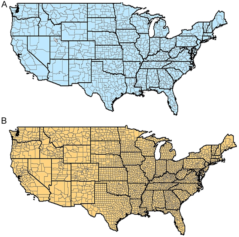
(A) Commuting zones; (B) U.S. counties

Measuring Risk and Return

We measure growth, or return, as the average of annual wage and salary employment growth over the most recent business cycle and risk as the standard deviation of growth over the business cycle. We measure risk and return over a business cycle, trough to trough, because risk and returns change with regional structural shifts over multiple business cycles (Spelman, 2006). Several studies examine growth and volatility over multiple and/or incomplete business cycles, but we use only the most recent complete business cycle because it is relevant for the entrepreneurship model, presented in the section Entrepreneurship Incentives, and we want to focus on the most recent employment portfolio. Regardless, results of this analysis held for all business cycles for which data are available. We measure risk and return over the 1991-2001 business cycle.² Data are obtained from the annual Bureau of Economic Analysis’ Regional Economic Information System (U.S. Dept. of Commerce, 1969-2005).

Returns to a regional employment portfolio are measured by the overall growth of job prospects, which is similarly in the interest of both workers and firms. Most related literature uses employment growth as the preferred measure of return, given its parallel with the underlying risk metric and the symmetric incentives for regional firms and workers (Barth et al., 1975; Chandra, 2002, 2003). We measure return as the average of annual wage and salary employment growth.

Regional employment portfolio studies use labor market risk as a measure of volatility of returns (Lande, 1994). Local workers (and employers) appreciate the greater certainty of stable growth. Such stability can translate into a more attractive environment for developing high-skill labor pools at relatively lower wages, as workers are willing to trade some wages for reductions in employment risk. Firms also appreciate such stability for the clearer planning horizons it provides, as well as the labor pool it can provide (Krugman, 1991). In parallel to returns, we measure risk as the standard deviation of annual wage and salary employment growth over the 1991-2001 business cycle.

Like most employment portfolio literature, we use employment-based measures of risk and return rather than income-based measures because using employment avoids spurious results because of regional differences in cost of living. More directly, employment is beneficial to the firm, workers, and the region as a whole as it signals greater productive capacity. The divergence of perspectives between firms (that appreciate lower wages, ceteris paribus) and workers (who appreciate precisely the opposite dynamic) reinforces the utility of a focus on employment growth. Finally, trends in employment tend to broadly follow income trends and other measures of return to a region, such as population and tax revenue, leading to our use of employment as the focal measure of return without loss of generality (Barth et al., 1975). In any case, we find the general relationship between risk and return is substantively identical whether measured by income or by employment.³

We use wage and salary employment rather than total employment because it is the most direct measure of opportunities in the formal labor market at a point in time, while also being unlikely to be a driver of the entrepreneurship measure introduced in the Entrepreneurship Incentives section of this article. The lack of such wage and salary employment opportunities—or volatility in such positions—increases the incentive to seek out self-employment in the future, a proposition that is formally tested. Wage and salary employment excludes those who are self-employed, allowing us to assess the incentive to engage in entrepreneurial self-employment as a reaction to prospects in the formal wage and salary sector.

Model

The model assumes regions (and workers) are risk averse. A worker will not take a job if another job, or entrepreneurial opportunity, has more favorable levels of risk and return. Similarly, a region will prefer to recruit firms with the goal of reaching favorable levels of risk and return—or it may opt to funnel its recruitment dollars into fostering entrepreneurship or other economic development policies and programs.

Before we can test whether the risk–return trade-off affects entrepreneurship, we must establish the existence of the risk–return trade-off for counties and CZs. Prior research established that the return-risk frontier is U shaped for states and metro areas and that the actual employment portfolios are associated with greater volatility is optimal—at a given time more regions are higher (more volatility) and more to the left (low growth) on the U-shaped frontier than necessary (Lande, 1994; Spelman, 2006). Simply plotting growth and risk for U.S. counties and CZs over the 1991-2002 business cycle weakly suggests a U-shaped relationship (Figure 2).

Figure 2.

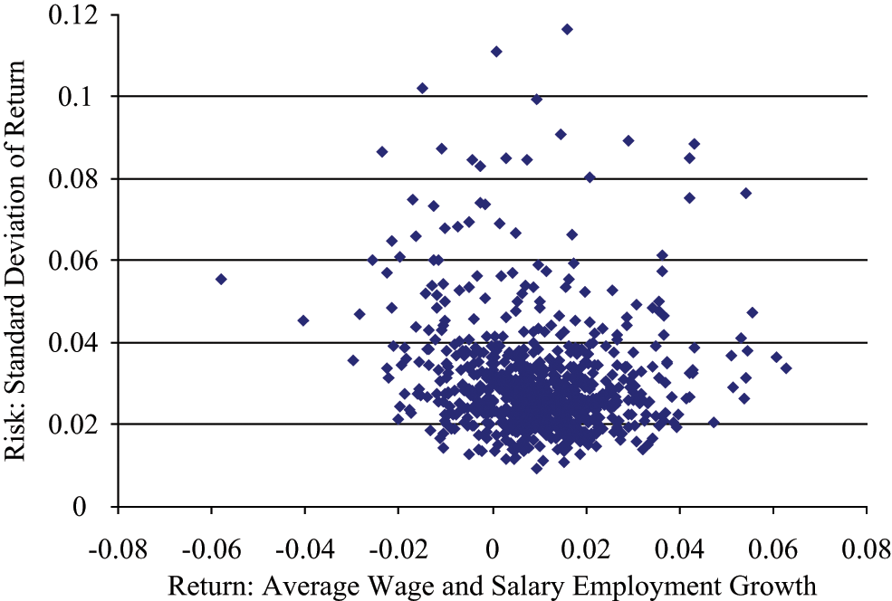
Commuting zone risk and return, 1991-2001 business cycle

We use stochastic frontier estimation to test for the quadratic relationship between risk and return (Chandra, 2002; Jondrow, Knox, Lovell, Materov, & Schmidt, 1982). The stochastic frontier estimation method permits a test of the nonconvexity of the employment portfolio frontier and estimates the parameters that define its shape. The alternative, a nonparametric method called data envelopment analysis, will produce a U-shaped frontier by construction (Spelman, 2006).

Stochastic frontier estimation is based on the assumption that the observations for each region lie on or within a frontier, creating one-sided disturbances. Aigner, Lovell, and Schmidt (1977) suggest two distributions for the one-sided disturbance, and we use the half-normal distribution because its specification best suits regional portfolio applications of stochastic frontier analysis. We specify the dependent variable and regressors according to Chandra (2002); σ_i is the standard deviation of the rate of growth for region i over a business cycle, G _i is the rate of growth for region i over the business cycle, and β₁ and β₂ are the parameters to be estimated. We specify the error term, ε_i, according to Jondrow et al. (1982). The estimated equation is as follows:

σ_{i} = α_{i} + β_{1} G_{i} + β_{2} G_{i}^{2} + ε_{i},

where $ε_{i} = υ_{i} - μ_{i}, υ_{i} \sim N (0, σ_{υ}^{2})$ and $ν_{i} \sim | N (0, σ_{ν}^{2}) |$ , hence, the half-normal distribution.

Except for the error term, ordinary least squares (OLS) results are unbiased and consistent. A nonlinear estimator, the maximum likelihood estimator, however, is more efficient than OLS; thus, we use maximum likelihood estimation to estimate Equation (1) using functions developed in FRONTIER 4.1. by Tim Coelli (see Battese & Coelli,1988). Empirically, we estimate Equation (1) using the variables Risk for σ_i and Growth for G_i.

Results

The empirical test confirms that there is a U-shaped trade-off between risk and return in county and CZ employment portfolios (Table 1). Plots confirm the global U shape. These results affirm work by Spelman (2006), Chandra (2002), and Lande (1994), who also found a quadratic relationship between growth and volatility in income or employment. That this relationship exists suggests that we can use risk and return to test whether employment portfolios affect entrepreneurship levels.

Table 1.

Test for U-Shaped Risk/Return Trade-off: Counties and Commuting Zones^a

Commuting zone estimation			County estimation
	Estimate	SE		Estimate	SE
Constant	0.012***	0.0005	Constant	0.011***	0.0004
Growth	−0.410***	0.041	Growth	−0.230***	0.022
Growth squared	12.9***	1.437	Growth squared	6.6***	0.115
N^b: 720			N^b: 2,959
Likelihood ratio test of the one-sided error = 174.41			Likelihood ratio test of the one-sided error = 899.14
Log likelihood = 2499.401			Log likelihood = 8271.677

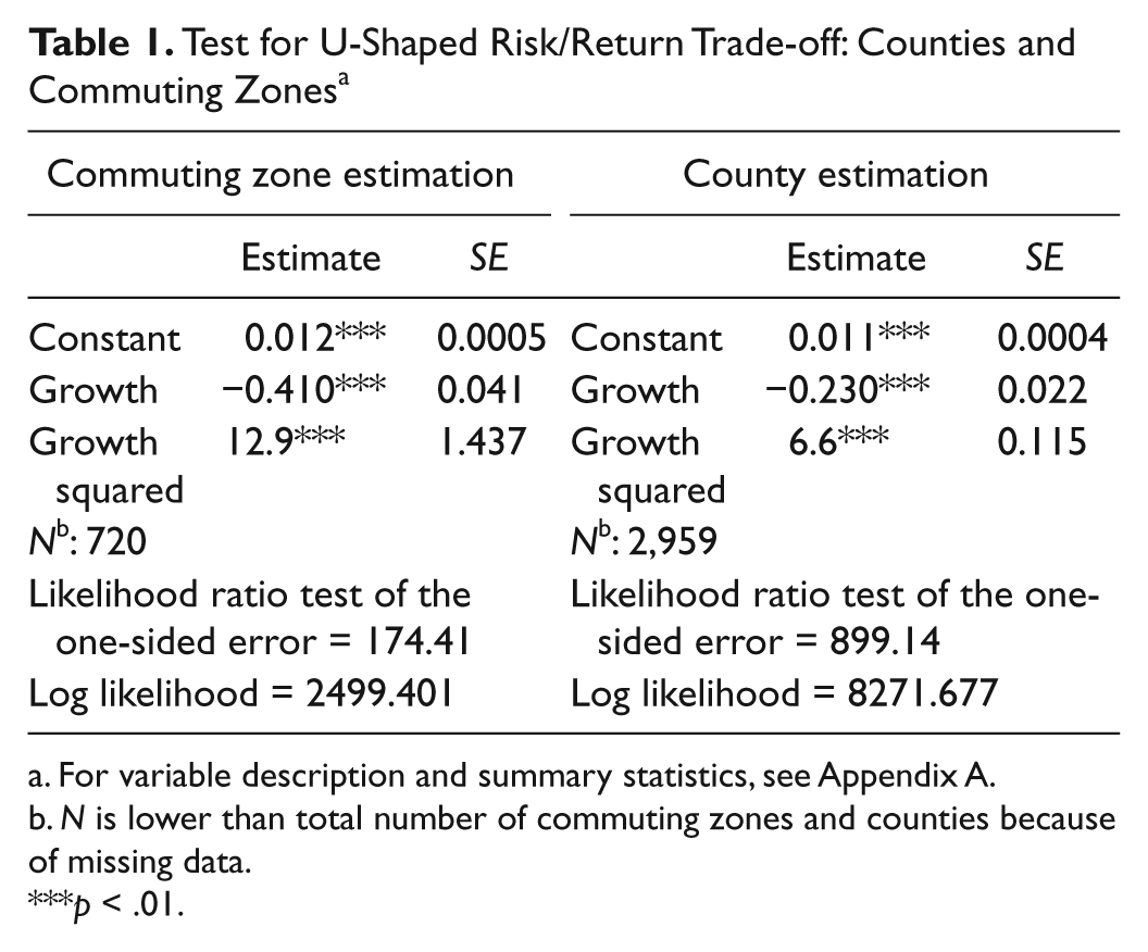
For variable description and summary statistics, see Appendix A.

N is lower than total number of commuting zones and counties because of missing data.

***

p < .01.

To the best of our knowledge, this analysis has only been successfully conducted at the substate level for metropolitan areas. Our finding is in opposition to Chandra (2003) who did not find statistically significant results for the stochastic test using European Union NUTS 3 (province) data.

Entrepreneurship Incentives

This section explores the likely supply-side influence of wage and salary employment portfolios established in the previous section, on engagement in entrepreneurial activity, measured empirically with self-employment and establishment birth rates, by empirically testing whether employment portfolios affect next period’s entrepreneurship levels. Economic development professionals and policy makers often fail to understand the region’s labor market behavior when developing business recruitment and entrepreneurship development policies and programs. Better understanding how risk and return incent nascent entrepreneurs will help with the implementation of better and more cost-effective programs to encourage economic growth and entrepreneurship.

Entrepreneurship and Local Labor Markets

We know of no research explicitly linking self-employment or entrepreneurship and local employment portfolios. Loveridge and Nizalov (2007) found a region needs to maintain a sufficiently large share of self employed entrepreneurs and other small businesses to enhance growth in other parts of the economy, suggesting the importance of the self-employed to the entire regional economy.

Parker (1996) provides motivation for our hypothesis. Using optimal control, he develops a model of self-employment among heterogeneous agents who maximize discounted expected utility under uncertainty. The model predicts that paid employment opportunities affect the decision to become an entrepreneur and that risk and risk aversion negatively affect the probability an agent becomes self-employed.

Parker (1996) finds evidence of people being pushed into self-employment because of lack of wage and salary job opportunities, often during recessions. This push into self-employment likely corresponds to the upper left of the employment portfolio when high wage and salary employment volatility and low growth conditions exist (see Figure 2). Parker also finds evidence of people being pulled into self-employment by high growth, developing markets, and increased disposable income—likely regions on the right of the U-shaped employment portfolio.

Both bodies of research hint at the explicit relationship between formal labor market risk and return and at the inherent incentives for both individual entrepreneurs and regional economies to value entrepreneurial business activity.

Defining Entrepreneurship for This Study

Defining entrepreneurship, “one of the most intriguing but equally elusive concepts in economics” (Peneder, 2009, p. 77), is a long-standing problem. A commonly accepted definition of entrepreneurship has failed to emerge (Gartner, 1988; Gartner & Shane, 1995; Luger & Koo, 2005), and defining and empirically measuring entrepreneurship, particularly at substate units of observation, is challenging and the topic of ongoing research.

Self-employment is measurable at substate units and is the most widely used proxy for entrepreneurship (Blanchflower & Oswald, 1998; Glaeser, 2007), particularly for economic development and regional research (Iversen, Jorgensen, & Malchow-Moeller, 2008). Because a definition of and measure for entrepreneurship does not exist, we adopt self-employment in part because proprietors satisfy the basic characteristic of entrepreneurs: owner-management and risk bearing (Henderson, Low, & Weiler, 2007). Furthermore, self-employment is a suitable proxy for entrepreneurship for the purposes of this article because it succinctly captures movement out of the formal wage and salary job market into self-employment, the two being exclusive of each other. Despite its wide use, self-employment is an imperfect measure of entrepreneurship. Self-employment is overly broad, failing to distinguish between innovative and noninnovative activity (e.g., nascent high-tech firms and lifestyle businesses). County-level data on innovative entrepreneurship do not yet exist, but are the topic of ongoing research (see Low, 2009).

As a robustness check, we also use establishment births as a metric for entrepreneurship. Establishment births is another widely used proxy for entrepreneurship (Acs & Mueller, 2008; Armington & Acs, 2002; Lee, Florida, & Acs, 2004), and some consider it a better measure of entrepreneurial activity than self-employment (Acs & Armington, 2003). Timely, regional data on establishment births, however, are more difficult to obtain, and births do not capture an individual’s movement into and out of the formal wage and salary job market like self-employment does, making coefficients of the establishment birth model more difficult to interpret.

Our principal dependent variable in the entrepreneurship model is the number of nonfarm proprietors normalized by total nonfarm employment, 2002. We also use the average nonfarm proprietorship rate 2002 to 2005 to ensure results are not specific to 2002. We measure the birth rate as new single-unit employer establishments, 2002 to 2003, normalized by 2002 employment.

Units of Observation

We model entrepreneurship at both the county and the CZ levels. County-level studies of entrepreneurship are becoming more common (Goetz & Rupasingha, 2009; Henderson et al., 2007), but to the best of our knowledge, no entrepreneurship studies have been conducted using CZs. Lee et al. (2004) find different factors drive new firm formation in Metropolitan Statistical Areas and Labor Market Areas (LMAs), likely because of the exclusion of the hinterland in LMAs, which suggests rural areas do influence the urban economy and should not be omitted from analysis, as is the case when Metropolitan Statistical Areas are the unit of observation. We extend existing analysis of entrepreneurship by using commuting sheds that are less aggregated than those used by Lee et al. (2004) and Armington and Acs (2002), but still provide a consistent set of local labor market agglomerations across both urban and rural areas.

Using smaller units of observation will improve the entrepreneurship model due to entrepreneurship’s pronounced regional and spatial dimension, which is partly because of entrepreneurial attitudes, financial capital, and human capital varying across space (Bull & Willard, 1993; Fritsch & Schmude, 2006). Additionally, most economic development is conducted at the local level (Bartik, 1991; Wasylenko, 1997); so, like employment portfolios, entrepreneurship policies should vary between regions.

Test and Model

We hypothesize the supply-side influence of wage and salary employment affects self-employment rates. We test this hypothesis by including employment portfolio components in an entrepreneurship model and testing if risk and return coefficients are different from zero. As Parker’s (1996) model suggests, we expect to find higher rates of self-employment where wage and salary employment volatility is high—thus we expect a positive coefficient on risk. The coefficient on return, or employment growth, could vary because the relationship between entrepreneurship and growth is quadratic. Self-employment is highest not only where growth is very low (e.g., entrepreneurship by necessity; Low, Henderson, & Weiler, 2005) but also where growth is very high because of thick markets, more income, and the associated demand-side opportunities for entrepreneurs (Goetz & Rupasingha, 2009; Parker, 1996). We expect a positive coefficient on growth squared, which is where growth is negative (far left on the U) or very high (far right on the U), entrepreneurship is higher.

Control variables

We test the hypothesis (above) using an entrepreneurship model containing a vector of explanatory variables widely used in entrepreneurship models and an additional vector of employment portfolio variables. We borrow heavily from Goetz and Rupasingha’s (2008) vector of explanatory variable, X, so we can focus the analysis on the inclusion of the employment portfolio variables, R, as determinants of entrepreneurship. Like others, we include demographic and regional characteristics (Acs, Armington, & Zhang, 2007; Goetz & Rupasingha, 2009; Lee et al., 2004).⁴ Demographic characteristics include financial capital and human capital. Regional characteristics include place-based characteristics and income-based characteristics. All variable descriptions, sources, and summary statistics are available in Appendix A.

Financial capital variables attempt to assess the ability of nascent proprietors to finance a new venture. The percentages of homeowners and median home value in a region are proxies for the ability to self-finance (Goetz & Freshwater, 2001; Goetz & Rupasingha, 2009). Bank deposits per capita has been used by others to gain insight on the availability of financial capital, particularly in rural areas (Garofolli, 1994; Goetz & Rupasingha, 2009; Low et al., 2005) and is a measure of how much money local banks have on hand for small business loans. Human capital control variables include percent of adults who are college educated and the percentage of noncollege graduates who did not graduate from high school or receive a GED. These human capital variables have been used to assess the relationship between human capital and entrepreneurship by Evans and Leighton (1989), Goetz and Freshwater (2001), Lee et al. (2004), and Goetz and Rupasingha (2009).

The percentage of persons residing in rural areas, or outside places with fewer than 2,500 people, controls for the strong relationship between proprietorship and rural regions. The Natural Amenity Scale (McGranahan, 1999) is an index of topography, weather, and water and is expected to control for the high levels of proprietorship in regions that are home to many “lone eagle” entrepreneurs who are attracted to the region by natural and scenic amenities (Carlino, Chatterjee, & Hunt, 2007; Kim, Marcouiller, & Deller, 2005).

We also include average wage and salary income and wage and salary income growth, rather than per capita income and per capita income growth, as Goetz and Rupasingha (2009) do. We use wage and salary income so that the focus remains on the wage and salary employment portfolio’s effect on the proprietorship rate. Wage and salary income captures the possibility that where wages are high, entrepreneurs may be drawn to participation in the formal job market—the opportunity cost of self-employment is higher. Furthermore, wage and salary income is a better measure of income because it is earned income and, unlike per capita income, excludes transfer payments, health care benefits, and so on.

Regressors are represented by average countywide or CZ-wide values so that each county or CZ proxies for the average characteristic of the potential pool from which proprietors are drawn (Goetz & Rupasingha, 2009).

Adding employment portfolio variables to the model

We add the employment portfolio variables to the entrepreneurship model to test the hypothesis that conditions in the wage and salary job market affect the level of entrepreneurship. Growth is defined as wage and salary employment growth over the 1991-2002 business cycle and we also use its square. Risk is defined as the standard deviation of employment growth over the 1991-2002 business cycle. Growth, its square, and Risk compose the vector of employment portfolio explanatory variables that is denoted in Equation (2) as the R vector.

Estimation issues

We use lagged explanatory variables to reduce the endogeneity bias, show that at least some of the causality flows from risk/return to proprietorship, and allow current entrepreneurship to be the longer term result of local workers considering and acting on a region’s formal wage and salary employment prospects over time. The estimated equation is the following:

Y_{t} = β R_{t - 1} + δ X_{t - 1} + ε_{t - 1} .

There is likely still endogeneity in the model because of the error term containing drivers of entrepreneurship and education; this simultaneity will cause results to be biased but consistent. Nevertheless, we estimate the linear model for counties and CZs using two-stage least squares (2SLS) (not shown) and found the results to be robust in coefficient sign and significance. Multicollinearity is not problematic in the model; the variance inflation factor (VIF) for each explanatory variable is less than 5. Equation (2) estimated by OLS suffers from heteroskedasticity of the error terms.⁵ The White–Huber correction is applied and standard errors re-estimated; results (not shown) remain consistent despite the correction.

Spatial issues

Heteroskedasticity in OLS models is one of the first indicators that the errors contain a spatial process. We suspect spatial processes likely exist because businesses, markets, and the labor force vary widely by region (Klein & Cook, 2006). Chinitz (1961) argues that entrepreneurship supply is a function of society, capital availability, and willingness to bear risk—all of which vary regionally. By controlling for spatial processes, noise is reduced, model fit is improved, and, importantly, heterogeneity is controlled for (Anselin, 1988).

Spatial error processes, or nuisance errors, can occur because of omitted spatially correlated variables or the value of adjacent observations moving together because of common or correlated unobservable variables. Experience tells us the county model likely suffers from spatial error, but developing a theory behind implementation of the spatial error model (SEM) is difficult because the errors are not because of some underlying process–rather a host of microprocesses. To improve model efficiency beyond OLS with a White–Huber correction, we use the spatial error model to control for spatially correlated disturbances between counties:

Y = β X + ε,

where ε = λWε + u, u ~ i.i.d.

Spatial lag processes occur because of interaction among neighbors. The use of the spatial lag model for CZs is appealing because CZs are small enough that networking and interaction between neighbors exists but big enough that nuisance errors do not override the spatial lag process, as is common in county-level models. When spatial lag processes are unaccounted for, coefficients can be biased and inconsistent, leading to the wrong sign on coefficients or invalid hypothesis testing. Spatial dependence of this type is most frequently incorporated into models using the spatial autoregressive (SAR) lag model:

Y = ρ W Y + β X + ε,

where ε ~ i.i.d. and W is an n × n matrix defining spatial unit interaction (Anselin, 1988).

There is very little formal guidance in the choice of the optimal spatial weights matrix (Anselin, 2008a). We use a first-order queen contiguity weights matrix because of the nature of spatial dependence and its suitability for use with irregular polygons. The weights matrix is row standardized to facilitate with interpretation and ease computational expense.

Lagrange multiplier (LM) tests are frequently used to test whether the spatial error or spatial lag process is present.⁶ For U.S. counties we find the lag and error LM tests are significant, thus we conduct robust LM tests. The robust LM test (error) is significantly different from zero and the robust LM (lag) test is insignificant, thus, the robust LM tests show preference for the SEM, confirming our hypothesis that nuisance errors exist in the U.S. counties model. For CZs, both LM tests are again significant, so we run the robust LM tests that suggested the spatial lag model is dominant over the spatial error for CZs, likely because there are less nuisance errors because of fewer and larger spatial units. Results of the LM tests affirm the expectations discussed; the CZ model is best suited to a SAR model.

Estimated model

The county model is estimated with the SEM model, Equation (3), using an optimal generalized method of moments covariance matrix robust to unspecified forms of heteroskedasticity detected in the OLS model with the Breusch–Pagan test. The CZ model is estimated with a SAR lag model, Equation (4), using a maximum likelihood estimation.

Results and Policy Implications

Hypothesis test results

We find evidence to reject the null hypothesis; that is, wage and salary employment risk and return do affect a region’s self-employment and establishment birth rates (Table 2). Significant coefficients on the variables of interest, risk, growth, and its square suggest that researchers should incorporate indicators of the regional employment portfolio into studies on the determinants of entrepreneurship. Finally, that employment opportunities and volatility affect the entrepreneurship level in a region suggests that wage and salary job opportunities (and industrial recruiting) must be considered in tandem with entrepreneurship development policies.

Table 2.

Regression Results, Y = Self-Employment, for County and CZ

	GMM estimation of SEM (error), U.S. Counties		MLE of SAR (lag), CZs
	County coefficient	SE	CZ Coefficient	SE
Constant	0.324***	0.018	0.151***	0.026
Risk	0.631***	0.101	1.062**	0.616
Growth	−0.188	0.144	−1.142***	0.315
Growth squared	7.288***	2.199	21.0***	6.990
% College educated	−0.026	0.036	−0.022	0.049
% High school dropouts	−0.197***	0.018	−0.095***	0.020
Bank deposits per capita	0.00001**	0.000007	0.002***	0.0003
% Home owners	0.061***	0.017	−0.081***	0.026
Median home value	0.0000005***	0.00000007	−0.0000001	0.00001
Natural amenities	0.005***	0.001	0.006***	0.0008
% Residing in rural place	0.127***	0.006	0.123***	0.008
Average income	−0.009***	0.001	0.00004	8.882
Income growth	−0.045***	0.007	0.010	0.021
λ LR test value = 31.204	0.160***
ρ			0.257***	0.042
Log likelihood	3546.4		1317.0
AIC	−7060.8		−2602.0
N ^a	2959		720

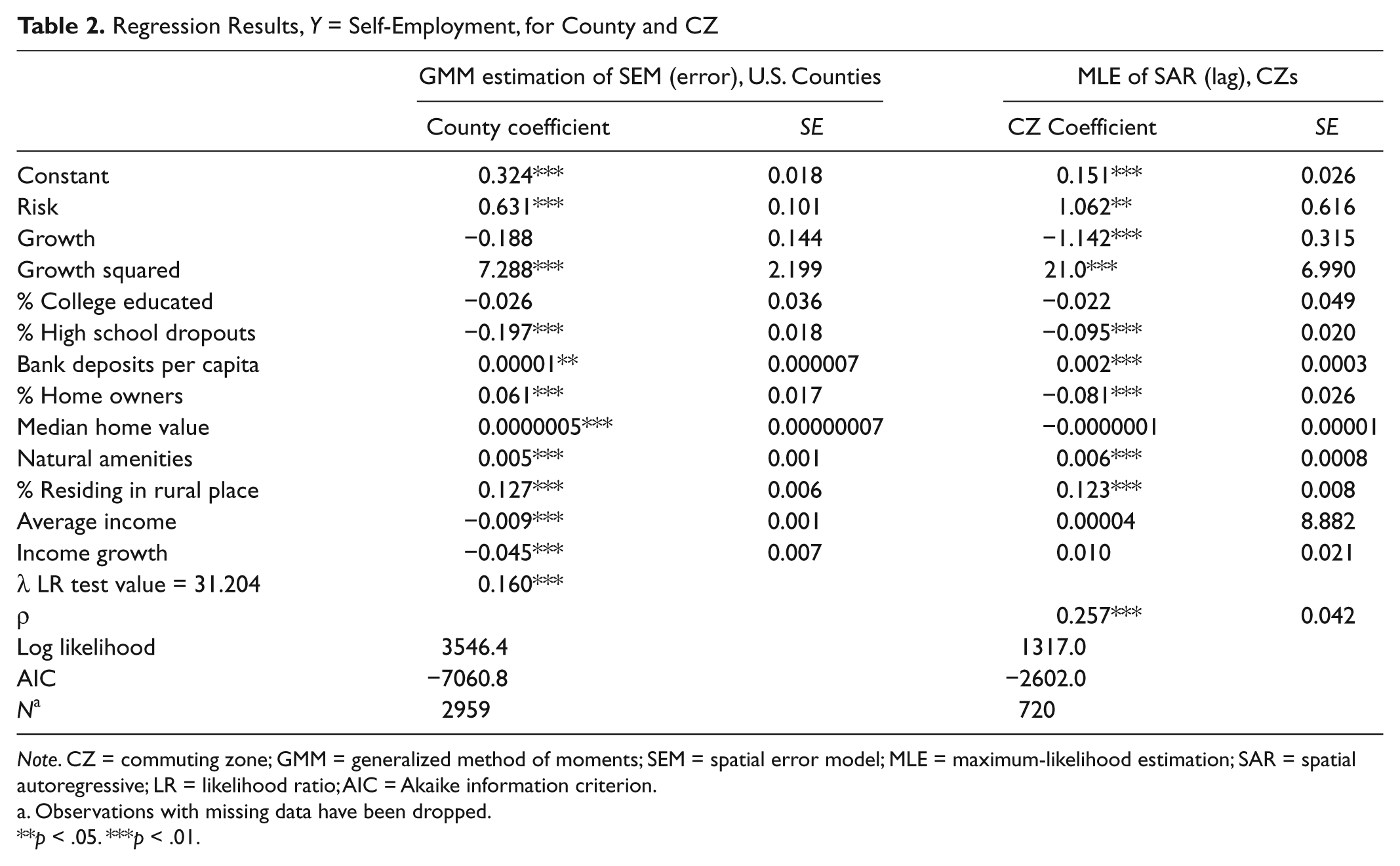
Note. CZ = commuting zone; GMM = generalized method of moments; SEM = spatial error model; MLE = maximum-likelihood estimation; SAR = spatial autoregressive; LR = likelihood ratio; AIC = Akaike information criterion.

Observations with missing data have been dropped.

p < .05. ***p < .01.

It is worth underscoring a cautionary note before proceeding with a discussion of the results. Because of the estimation methods employed, estimated coefficients cannot be interpreted in the same straightforward manner as OLS results. For example, in a linear OLS estimation, we can interpret a coefficient as the difference in the predicted value of Y, self-employment, for each unit difference in X, say a standard deviation difference in Risk, ceteris paribus. This interpretation is more complex in spatial econometric models because of nonlinear estimation methods, the spatial multiplier effect, and spatial connectivity—a change in an explanatory variable in region i will have a direct impact on region i as well as an indirect impact on other regions. For a detailed discussion of these complexities, we refer the reader to Anselin (2003) or Le Sage and Pace (2009). Because of the complications associated with interpreting coefficients in spatial econometric models, we focus rather on assessing whether results are reasonable and providing a general sense of the magnitude of test results.

Results of the test on Risk align with our intuition that when wage and salary employment volatility is higher, more people are self-employed in the next period—likely a response to labor market conditions. The effect of wage and salary employment volatility on self-employment is relatively large. In the county-level model, a 1 standard deviation increase in risk increases the self-employment rate by 63% (Table 2), an expectedly large result. Given the complications associated with interpreting spatial econometric coefficients, this magnitude must be considered judiciously; however, the linear OLS estimate was in a similar range at 70%. For CZs, the increase is 106%, likely because the spatial lag model, indicated for CZs, includes both direct and indirect effects. In short, test results suggest that volatility in the wage and salary job market is associated with more workers being self-employed in the next period—or being their own boss, whether out of necessity or because of opportunity.

Results suggest an inverse relationship between wage and salary employment growth and the self-employment rate dominates (Table 2). The spatial econometric coefficient suggests that the hypothesized relationships exist but are relatively smaller than the Risk results. In the CZ model, predicted self-employment is 1.1% higher when wage and salary employment growth decreases by 1%; that is, when jobs decrease by 1%, the next period’s self-employment rate is 1.1% higher. The square of wage and salary growth is positive and significant, as expected, suggesting that the growth affect occurs at an increasing rate. Wage and salary employment growth was insignificant in the county-level model, likely because counties are a less appropriate areal unit than CZs. Growth squared is significant and positive, as expected, suggesting that the wage and salary employment rate decreases at an increasing rate.

Coefficient signs and significance are the same in the model of establishment births (Appendix B). Coefficient magnitudes, however, suggest that births are less responsive to wage and salary employment risk and growth in the previous period than is self-employment. Interpretation of coefficients in the employer establishment birth model is less meaningful than in the self-employment model because births do not capture individuals’ movement between self-employment and wage and salary employment as succinctly as self-employment. Finally, tests using self-employment for 2002-2005 yielded similar results, suggesting results are not specific to 2002.

Demographic variables

The coefficient on the high school dropout rate was negative and significant (.01), suggesting that efforts to decrease the high school dropout rate may increase proprietorship. Percentage with a college degree was statistically insignificant, although others have found a positive and significant coefficient (Henderson et al., 2007). The test of homeownership as a proxy for capital availability was inconclusive; however, bank deposits per capita has a positive and significant (.01) driver of entrepreneurship in both counties and CZs. This result suggests that efforts to improve access to small amounts of capital may foster entrepreneurship. An example would be establishing a revolving loan fund for nascent entrepreneurs in the region.

Regional variables

Regional variables are place based and income based. The only place-based variable that has policy implications is the Natural Amenity Scale because rurality is difficult to influence with policy. In both regressions, the coefficient on natural amenities has a positive and significant (.01) coefficient, which was expected because recent literature has found natural amenities and landscape to influence entrepreneurship (Henderson et al., 2007). Prior research has also suggested that amenities are necessary to attract and retain skilled professionals (Gale, 1998). Although amenities cannot be changed in the short term, regions can influence the appearance and accessibility of their environment. Mountaintop strip mining may negate the amenity value of mountains in West Virginia. Planting trees, providing recreational access to buffer strips, and rails to trails projects may increase the amenity value of a place. Income-based variables were insignificant in the CZ model, but we find income and income growth to be negatively associated with the proprietorship rate in the county model at the .01 level of significance. This could be because the nonfarm proprietor income is below wage and salary income.

Conclusions

We find that risk and return in the wage and salary job market affect self-employment and, to a lesser extent, establishment birth rates, in the next period. In uniting two previously disparate literatures, this research makes contributions to both the entrepreneurship and employment portfolio literature as they relate to local labor market research and development. The research is the first known to connect regional employment portfolio theory with entrepreneurship, particularly in terms of the incentive to pursue self-employment given the risk/return patterns of local wage and salary positions. Second, this research represents the first consistently successful application of portfolio theory to submetropolitan economies such as counties and CZs, with CZs in particular allowing both broader and deeper insights into local labor market interactions through their commuting shed agglomerative lens. Furthermore, by better understanding the determinants of entrepreneurship and realizing that wage and salary employment opportunities can affect entrepreneurship incentives, policy makers can better foster entrepreneurship in their region. Entrepreneurial clubs (Green, Wise, & Armstrong, 2007), workshops and training (Camp, 2005), financial capital (Garofolli, 1994), and entrepreneurial development systems (Lyons & Hamlin, 2001) may increase entrepreneurship incentives. A better understanding of how job prospects affect entrepreneurship may also provide information to better allocate economic development dollars between recruitment and entrepreneurship.

The spatial detail of this research also empowers regional decision making rather than all regions following a blanket policy (Klein & Cook, 2006). If a region is above and left of the optimal frontier, leaders can allocate scarce economic development dollars differently with the goal of reducing volatility and/or increasing employment growth. This result is important because a lot of economic development policy in the United States is conducted at the local level—meaning, for the first time, portfolio analysis of labor markets can be used by economic development practitioners rather than having to use less specific state results.

This research begets more research. Focusing on the differences in entrepreneurship incentives between urban and rural counties and CZs may explain some of the results of this research. Future research will examine whether entrepreneurship can be used to decrease volatility and/or increase growth while incorporating industry sectors into the analysis—the idea being that regions encourage entrepreneurship in sectors that behave counter-cyclically to existing industry, which would further decrease regional employment portfolio volatility.

Footnotes

Appendix B

Appendix A

Variable Description and Summary Statistics

	Mean	SD	Minimum	Maximum	Description
Risk	0.032	0.027	0.006	1.06	Standard deviation of annual wage and salary employment growth, 1991-2002 business cycle^a
Growth	0.014	0.018	−0.052	0.422	Average of annual wage and salary employment growth, 1991-2002 business cycle^a
Growth squared	0.001	0.004	0	0.178	Growth (see above), squared^a
% College educated	0.133	0.063	0.037	0.534	Percentage of adults >25 years with a 4-year college degree^b
% High school dropouts	0.346	0.103	0.074	0.734	Percentage of adults >25 years without a 4-year degree who have not completed high school^b
Bank deposits per capita	36.6	213.2	0	6875.8	Bank deposits ($1,000) per capita, Federal Deposit Insurance, 1990
Average income	17.34	3.713	9.829	40.526	Wage and salary income ($1,000) divided by population^a, 1990
Natural amenities	0.055	2.313	−6.4	11.17	McGranahan’s (1999) Natural Amenity Scale, U.S. Department of Agriculture, Economic Research Service
% Home owners	0.618	0.091	0.101	0.827	Percentage of residences that are owner occupied^b
Median home value	52,353	32,107	14,999	500,001	Median home value ($)^b
% Residing in rural place	0.637	0.291	0	1	Farm plus nonfarm rural residentsdivided by population^b
Income growth	0.753	0.564	−0.303	16.052	Wage and salary income growth^a, 1991-2002
Self-employment rate	0.24	0.091	0.029	0.678	Nonfarm proprietor employment over nonfarm employment^a, 2002
Establishment birth rate	9.417	6.039	0	96.774	Single-unit employer establishment births 2002-2003 over (2002 employment/1,000), U.S. Census Bureau

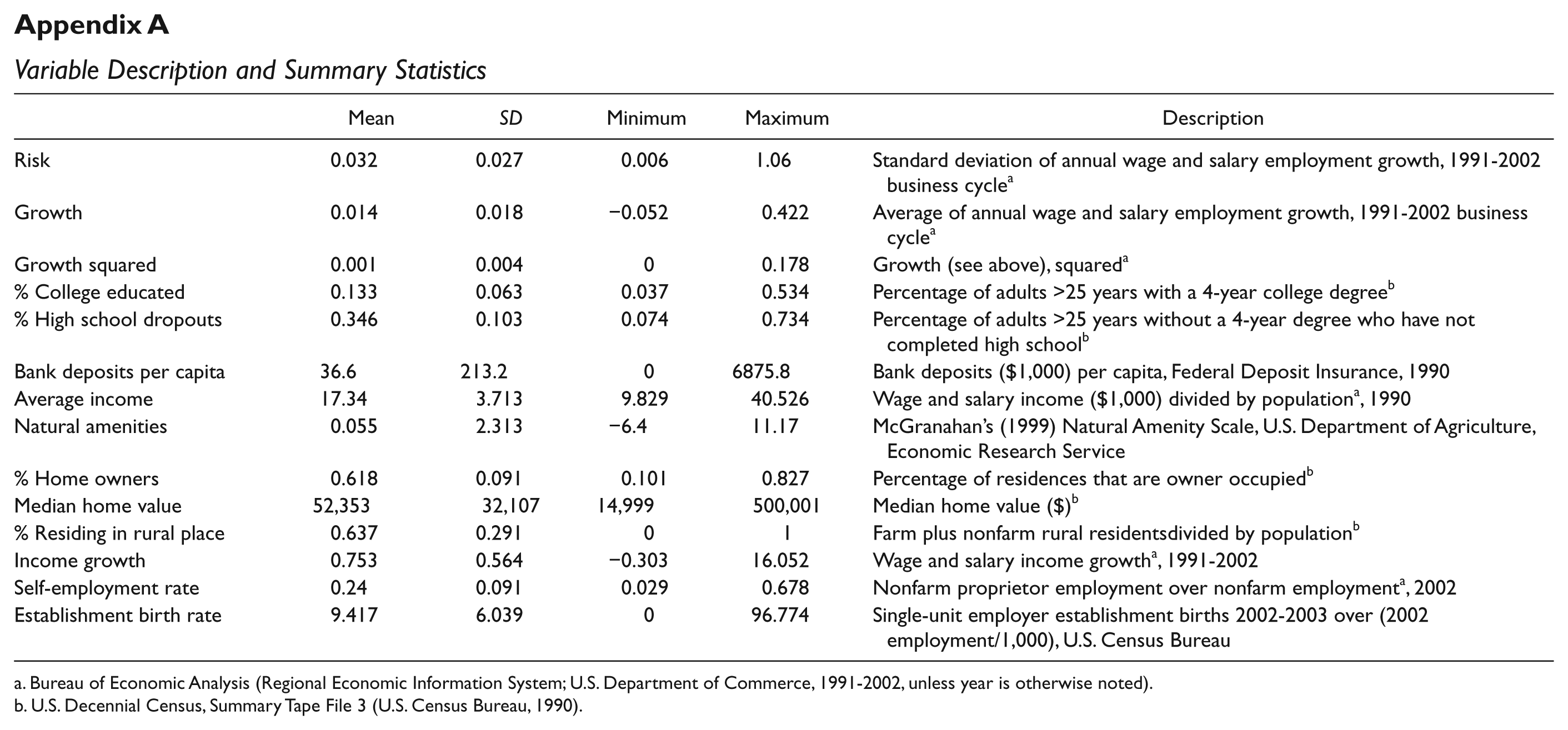
Bureau of Economic Analysis (Regional Economic Information System; U.S. Department of Commerce, 1991-2002, unless year is otherwise noted).

U.S. Decennial Census, Summary Tape File 3 (U.S. Census Bureau, 1990).

Authors’ Note

The views expressed here are those of the authors and may not be attributed to the Economic Research Service, the U.S. Department of Agriculture, or Colorado State University.

Declaration of Conflicting Interests

The author(s) declared no potential conflicts of interest with respect to the research, authorship, and/or publication of this article.

Funding

The author(s) received no financial support for the research, authorship, and/or publication of this article.

Notes

Bios

Sarah A. Low is an economist with the U.S. Department of Agriculture, Economic Research Service, in the Farm and Rural Business branch. Her research focuses on rural economic development, particularly entrepreneurship, labor, and spatial analysis.

Stephan Weiler is a professor of Economics and Research Associate Dean at Colorado State University. His research agenda spans a range of economic development issues broadly unified by the principals of informational asymmetry to understand divergent outcomes.

References

Acs

Armington

(2003). Endogenous growth and entrepreneurial activity in cities. Retrieved from http://www.unm.edu/~asalazar/Kauffman/Entrep_research/e_cities.pdf

Acs

Armington

Zhang

(2007). The determinants of new-firm survival across regional economies. Papers in Regional Science, 86, 367-391.

Acs

Mueller

(2008). Employment effects of business dynamics: Mice, gazelles and elephants. Small Business Economics, 30, 85-100.

Aigner

Lovell

C. A. K.

Schmidt

(1977). Formulation and estimation of stochastic frontier production function models. Journal of Econometrics, 6, 21-37.

Anselin

(1988). Spatial econometrics: Methods and models. Dordrecht, Netherlands: Kluwer Academic.

Anselin

(2003). Spatial exernalities, spatial multipliers, and spatial econometrics. International Regional Science Review, 26, 153-166.

Anselin

(2008a, July). Model specification lecture. Presented at the European Regional Science Association Summer School, Pécs, Hungary.

Anselin

(2008b). Spatial regression. In Fotheringham

A. S.

Rogerson

(Eds.), The SAGE handbook of spatial analysis (pp. 255-276). London, England: Sage.

Armington

Acs

(2002). The determinants of regional variation in new firm formation. Regional studies, 36, 33-45.

10.

Barry

Kearney

(2006). MNEs and industry structure in host countries: A portfolio analysis of Irish manufacturing. Journal of International Business Studies, 37, 392-406.

11.

Barth

Kraft

Wiest

(1975). A portfolio theoretic approach to industrial diversification and regional employment. Journal of Regional Science, 15, 9-15.

12.

Bartik

(1991). Who benefits from state and local economic development policies? Kalamazoo, MI: W. E. Upjohn Institute for Employment Research.

13.

Battese

Coelli

(1988). Prediction of firm-level technical efficiencies with a generalized frontier production function and panel data. Journal of Econometrics, 38, 387-399.

14.

Blanchflower

Oswald

(1998). What makes an entrepreneur. Journal of Labor Economics, 1(16), 26-60.

15.

Bull

Willard

(1993). Toward a theory of entrepreneurship. Journal of Business Venturing, 8, 185-195.

16.

Camp

S. M.

(2005). The innovation-entrepreneurship nexus: A national assessment of entrepreneurship and regional economic growth and development (Small Business Research Summary No. 256). Powell, OH: Advanced Research Technologies.

17.

Carlino

Chatterjee

Hunt

(2007). Urban density and the rate of innovation. Journal of Urban Economics, 61, 389-419.

18.

Carlino

DeFina

Sill

(2004). On the stability of employment growth: A postwar view from the U.S. states. Philadelphia, PA: Federal Reserve Bank of Philadelphia.

19.

Chandra

(2002). A test of the regional growth-instability frontier using state data. Land Economics, 78, 442-462.

20.

Chandra

(2003). Regional economy size and the growth-instability frontier: Evidence from Europe. Journal of Regional Science, 43, 95-122.

21.

Chinitz

(1961). Contrasts in agglomeration: New York and Pittsburgh. American Economic Review, 51, 279-289.

22.

Conroy

(1974). Alternative strategies for regional industrial diversification. Journal of Regional Science, 14, 31-46.

23.

Evans

Leighton

(1989). The determinants of changes in U.S. self-employment, 1968-1987. Small Business Economics, 1, 111-119.

24.

Fritsch

Schmude

(Eds.). (2006). Entrepreneurship in the region. New York, NY: Springer.

25.

Gale

H. F.

(1998). Rural manufacturing on the crest of a wave: Count data analysis of technology adoption. American Journal of Agricultural Economics, 80, 347-357.

26.

Garofolli

(1994). New firm formation and regional development: The Italian case. Regional Studies, 28, 381-393.

27.

Gartner

(1988). Who is an entrepreneur? is the wrong question. American Journal of Small Business, 12(4), 11-32.

28.

Gartner

Shane

(1995). Measuring entrepreneurship over time. Journal of Business Venturing, 10, 283-301.

29.

Glaeser

(2007). Entrepreneurship and the city (NBER Working Paper No. 13551). Retrieved from http://www.economics.harvard.edu/faculty/glaeser/files/ENTREPRENEURSHIP%20AND%20THE%20CITY%20-%2010.17.07.pdf

30.

Goetz

Freshwater

(2001). State-level determinants of entrepreneurship and a preliminary measure of entrepreneurial climate. Economic Development Quarterly, 15, 58-70.

31.

Goetz

Rupasingha

(2009). Determinants of growth in non-farm proprietor densities in the US, 1990-2000. Small Business Economics, 32, 425-438.

32.

Green

Wise

Armstrong

(2007, October). Inventor and entrepreneur clubs: Investment in an innovative approach to entrepreneurship. Paper presented at the Frameworks for Entrepreneurship Research in Food, Agriculture, Natural Resources and Rural Development: A National Conference on Entrepreneurship Research, Kansas City, MO.

33.

Hammond

Thompson

(2004). Employment risk in U.S. metropolitan and nonmetropolitan regions: The influence of industrial specialization and population characteristics. Journal of Regional Science, 44, 517-542.

34.

Henderson

Low

S. A.

Weiler

(2007). The drivers of regional entrepreneurship in rural and metro areas. In Walzer

(Ed.), Entrepreneurship and local economic development (pp. 81-102). Lanham, MD: Lexington Books.

35.

Iversen

Jorgensen

Malchow-Moeller

(2008). Defining and measuring entrepreneurship. Foundations and Trends in Entrepreneurship, 4(1), 1-63.

36.

Jackson

(1984). An evaluation of alternative measures of regional industrial diversification. Regional Studies, 18, 103-112.

37.

Jondrow

Knox

Lovell

Materov

Schmidt

(1982). On the estimation of technical inefficiency in the stochastic fronter production function model. Journal of Econometrics, 19, 233-238.

38.

Kim

K.-K.

Marcouiller

D. W.

Deller

S. C.

(2005). Natural amenities and rural development: Understanding spatial and distributional attributes. Growth and Change, 36, 273-297.

39.

Klein

Cook

(2006). T. W. Schultz and the human-capital approach to entrepreneurship. Review of Agricultural Economics, 28, 344-350.

40.

Kort

(1981). Regional economic instability and industrial diversification in the U.S. Land Economics, 57, 596-608.

41.

Krugman

(1991). Geography and trade. Cambridge: MIT Press.

42.

Lande

(1994). Regional industrial structure and economic growth and instability. Journal of Regional Science, 34, 343-360.

43.

Le Sage

Pace

R. K.

(2009). Introduction to spatial econometrics. Boca Raton, FL: CRC Press.

44.

Lee

Florida

Acs

(2004). Creativity and entrepreneurship: A regional analysis of new firm formation. Regional Studies, 38, 879-891.

45.

Loveridge

Nizalov

(2007). Operationalizing the entrepreneurial pipeline theory: An empirical assessment of the optimal size distribution of local firms. Economic Development Quarterly, 21, 244-262.

46.

Low

S. A.

(2009). Defining and measuring entrepreneurship for regional research: A new approach (Unpublished dissertation). University of Illinois at Urbana-Champaign.

47.

Low

S. A.

Henderson

Weiler

(2005). Guaging a region’s entrepreneurship, Economic Review. Kansas City, MO: Federal Reserve Bank of Kansas City.

48.

Luger

M. I.

Koo

(2005). Defining and tracking business start-ups. Small Business Economics, 24, 17-28.

49.

Lyons

S. T.

Hamlin

R. E.

(2001). Creating an economic development action plan. New York, NY: Praeger.

50.

Markowitz

(1952). Portfolio selection. Journal of Finance, 7, 77-91.

51.

McGranahan

D. A.

(1999). Natural amenities drive rural population change (Agricultural Economic Report No. ARE781). Washington, DC: Economic Research Service, U.S. Department of Agriculture.

52.

Parker

(1996). A time series model of self employment under uncertainty. Economica, 63, 469-475.

53.

Peneder

(2009). The meaning of entrepreneurship: A modular concept. Journal of Industry, Competition and Trade, 9, 77-99.

54.

Schumpeter

(1975). Capitalism, socialism, and democracy. New York, NY: Harper. (Original work published 1942)

55.

Spelman

(2006). Growth, stability, and the urban portfolio. Economic Development Quarterly, 20, 299-315.

56.

Tolbert

Sizer

(1996). U.S. commuting zones and labor market areas: A 1990 update. U.S. Department of Agriculture, Economic Research Service.

57.

U.S. Census Bureau. (1990). Census ’90. Retrieved from http://www.census.gov/main/www/cen1990.html

58.

U.S. Department of Commerce. (1969-2005). Regional Economic Information System [Data set]. Retrieved from http://www.ciesin.org/datasets/reis/about.bea.information.html

59.

Wasylenko

(1997). Taxation and economic development: The state of the economic literature. New England Economic Review, March/April, 37-52.

60.

Wundt

(1992). Reevaluating alternative measures of industrial diversity as indicators of regional cyclical variations. Review of Regional Studies, 22, 59-73.