Solving the Nonresponse Problem With Sample Matching?

Survey Sampling

The development of the theory of survey sampling started around the year 1895. In this year, Kiaer proposed his representative method, which can be seen as a form of quota sampling. Unfortunately, his approach lacked a formal theory of inference. Therefore, it was not possible to establish the accuracy of estimates. It was Bowley (1906, 1926), who solved this problem by proposing probability sampling. He showed that for large samples, selected at random with equal probabilities from a population, estimators had an approximately normal distribution. So it became possible to compute variances. Neyman (1934) extended this theory by introducing the concept of the confidence interval. Neyman also showed that Kiaer’s representative method based on purposive sampling failed to provide satisfactory estimates. Finally, Horvitz and Thompson (1952) showed in their seminal paper that probability sampling always allows for constructing unbiased estimators if all selection probabilities are positive and known.

There are various ways of selecting a sample for a survey; but over the years, it has become clear that a scientifically sound way to do this is by means of probability sampling. The paradigm of probability sampling has shown to work well in social research, official statistics, and market research. It has allowed researchers to produce well-founded and reliable survey results.

There are developments, however, making application of the probability sampling paradigm not so straightforward any more. The first development is decreasing response rates. This affects the representativity of survey response and hence may lead to biased estimates of population characteristics. The second development is the increased popularity of self-selection (opt-in) web surveys. These are surveys that are just put on the web. There is no sampling design. Everybody can complete the survey questionnaire. This comes down to a form of sampling in which all selection probabilities are unknown. Therefore, the theory of Horvitz and Thompson cannot be applied. It is impossible to construct unbiased estimators in a simple and straightforward way.

This article explores the use of matched samples as an alternative for estimators based on surveys suffering from a substantial amount of nonresponse. The focus is on reducing nonresponse bias of estimates in general population surveys. Samples for these surveys often have a substantial size, thereby making bias a more important component of the accuracy of estimates than sample variance.

Survey Challenges

Two types of nonresponse can be distinguished: unit nonresponse and item nonresponse. Unit nonresponse means that no information at all is obtained from a number of elements in the sample. Their questionnaire forms remain completely empty. Item nonresponse refers to the situation in which only some questions are left unanswered, because respondents do not know the answer or do not want to give an answer. The focus is here on unit nonresponse, which will simply be denoted by nonresponse.

Nonresponse is often modeled by assigning an (unknown) probability of response to every element in the population. As a consequence, the probability of getting data from specific elements depends on the following two random processes: the (known) sample selection mechanism and the (unknown) response mechanism.

Since the probability of getting an observation is unknown, the theory of Horvitz and Thompson cannot be applied. Hence, there is no straightforward way to compute unbiased estimates. Nonresponse rates have increased in many countries over time and this increases the risk of drawing wrong conclusions from a survey.

One can attempt to remove or reduce the bias due to nonresponse by applying some kind of weighting adjustment technique (see, e.g., Bethlehem, Cobben, & Schouten, 2011 or Särndal & Lundström, 2005). Another correction technique is to estimate the response probabilities and include them in the Horvitz–Thompson estimation procedure. There is, however, no guarantee that these correction techniques will fully remove the bias caused by nonresponse.

Another development in survey methodology is the emergence of online data collection. Web surveys (including surveys taken from web panels) quickly became very popular, particularly in the world of market research. This is not surprising, as it is a cheap and fast means of getting access to a large group of people.

Questionnaires of web surveys can be distributed at very low costs. No interviewers are needed and there are no mailing and printing costs. Surveys can be launched very quickly. Little time is lost between the moment the questionnaire is ready and the start of the fieldwork. And web surveys offer new, attractive possibilities, such as the use of multimedia (audio, pictures, animation, and video).

A serious problem of web surveys is often the lack of a proper sampling frame. Such frames may exist for a survey among employees of a large company or among students of a university, but there is no list of email addresses of all people in the general population. There is also not something like random digit dialling (RDD), which may be applied for telephone surveys. These frame problems cause many web surveys to be based on self-selection instead of probability sampling. Self-selection means that it is completely left to people to decide to participate in a survey. Respondents are those people who happen to have Internet, visit the website, and decide to participate in the survey. Self-selection can be modeled by assigning every element in the target population a certain unknown participation probability. Since these probabilities are unknown, it is not possible to construct unbiased estimators for population characteristics. Self-selection web surveys may suffer from more problems, that is, people who participate more than once, respondents from outside the target population, and groups of people who together attempt to manipulate the outcomes of the survey. Examples of manipulation of political polls are given by Bronzwaer (2012) and Bethlehem (2014).

For these reasons, many survey researchers consider self-selection surveys and panels out of the question for compiling accurate statistics about the general population. Indeed, a special task force of American Association of for Public Opinion Research concluded that “Researchers should avoid nonprobability online panels when one of the researcher objectives is to accurately estimate population values” (see Baker et al., 2010).

Matched Samples

With increasing nonresponse rates, one may wonder, however, to what extent the probability sampling paradigm can still be applied. Selection probabilities depend on both the known sample selection mechanism and the unknown response mechanism. Therefore, the overall selection probabilities are unknown. In this respect, a probability sample survey with nonresponse resembles a self-selection survey.

Rivers (2007) states that many telephone polls in the United States have response rates of no more than 20%. And web surveys based on probability sampling have a response rate of at most 40% in many countries. This raises the fundamental question whether valid statistical inference is still possible in such situations.

As a solution for the increasing nonresponse problems in probability-based surveys, Douglas Rivers has proposed a different way of data collection, which is a form of sample matching. His approach is described in, for example, Rivers (2007), Vavreck and Rivers (2008), and Rivers and Bailey (2009). Application of sample matching requires two ingredients:

A sampling frame that covers the target population of the survey. A probability sample is selected from this frame. The sampling frame must contain a set of auxiliary variables or it must be possible to uniquely link another data source of auxiliary variables (e.g., a register) to this frame.

The idea is to select a probability sample from the sampling frame. The selected people are not asked to complete a questionnaire form, as this would lead to high nonresponse rates. Instead, people are located in the panel who resemble the selected persons. These panel members are invited to complete the questionnaire. The response rate will be high as the panel contains people who agreed to complete survey questionnaires regularly.

The main issue of sample matching is to find people in the panel who resemble the selected people in the sampling frame as much as possible. The auxiliary variables are used for this.

Rivers tested his approach in the Cooperative Congressional Election Study. He concluded that sample matching is capable of removing nonresponse bias in this survey. He also concluded that his estimates were less biased than those of surveys based on RDD recruitment.

This article investigates the properties of sample matching in some more detail. The focus is on reducing the nonresponse bias. It should be noted that many, if not all, nonresponse correction techniques make use of a set of auxiliary variables. It will be shown that these techniques are only successful if these auxiliary are capable of completely explaining participation behavior of the elements and of the surveys variables.

Using simulated data, it is explored under which conditions sample matching may work. The second section presents the mathematical framework. It shows what the effects of nonresponse are on the bias of estimates. It also describes how self-selection surveys can produce biased estimates. The third section is about the basics of sample matching. It stresses the important role of auxiliary variables in matching persons in the sampling frame to persons in the panel. The fourth section gives an account of a small simulation study. It shows that sample matching is no guarantee for success. The fifth section compares sample matching with some more traditional sampling approaches, that is, selecting a stratified sample from the panel and selecting a simple random sample from the panel followed by post-stratification. The final sixth section discusses the advantages and disadvantages of the various approaches.

Sampling From a Finite Population

Let the finite target population U of the survey consist of a set of N identifiable elements, which are labeled 1, 2, … , N. Associated with each element, k is an unknown value Y_k of the target variable. There are many population characteristics that may be of interest to a researcher, but here it is assumed that objective of the sample survey is estimation of the population mean

Y ˉ = 1 N ∑ k = 1 N Y k .

1

To estimate this population parameter, a probability sample of size n is selected without replacement. The sample can be represented by a set a ₁, a ₂, … , a_N of indicators. The kth indicator a_k assumes the value 1 if element k is selected in the sample; and otherwise, it assumes the value 0. The first-order inclusion probability of element k is defined by π _k = E(a_k ), for k = 1, 2, … , N.

The Horvitz–Thompson estimator is defined by

y ˉ H T = 1 N ∑ k = 1 N a k Y k π k .

2

Note that most sample quantities are denoted by lowercase symbols and population quantities by uppercase symbols. It can be shown that estimator (2) is an unbiased estimator of the population mean (because E(a_k ) = π _k ). In the case of simple random sampling, all first-order inclusion probabilities are equal, that is, π _k = n/N. Then, the Horvitz–Thompson estimator reduces to the sample mean

y ˉ H T = 1 n ∑ k = 1 N a k Y k .

3

Nonresponse in a Simple Random Sample

Suppose there is nonresponse in the survey. It is assumed that each element k in the population has a certain, unknown probability ρ _k of response. If element k is selected in the sample, a random mechanism is activated that results with probability ρ _k in response and with probability 1 − ρ _k in nonresponse. Under this model, a set of response indicators R ₁, R ₂, … , R_N can be introduced, where R_k = 1 if the corresponding element k responds, and where R_k = 0 otherwise. So, P(R_k = 1) = ρ _k , and P(R_k = 0) = 1 − ρ _k .

The survey response only consists of those elements k for which a_k = 1 and R_k = 1. Hence, the number of available cases is equal to

n R = ∑ k = 1 N a k R k .

4

Note that this realized sample size is a random variable. Likewise, the number of nonrespondents is equal to

n N R = ∑ k = 1 N a k ( 1 − R k ) ,

5

where n = n_R + n_NR . The values of the target variable only become available for the n_R responding elements. Due to nonresponse, selection, probabilities changed. The probability of getting a value from element k is now ρ _k π _k instead of π _k . Consequently, the Horvitz–Thompson estimator would be:

y ˉ H T = 1 N ∑ k = 1 N a k R k Y k ρ k π k .

6

This estimator cannot be computed in practice, because the response probabilities ρ_k are unknown. As a way out, Bethlehem (1988) suggests replacing these probabilities by the unbiased estimate of the mean response probability, defined by

r ˉ H T = 1 N ∑ k = 1 N a k R k π k .

7

This leads to the modified Horvitz–Thompson estimator

y ˉ H T ∗ = 1 N ∑ k = 1 N a k R k Y k π k r ˉ H T .

8

In case all selection probabilities are equal, expression (8) reduces to the simple response mean. Bethlehem (2009) shows that the expected value of this estimator is approximately equal to

E ( y ˉ R ) ≈ 1 N ∑ k = 1 N ρ k ρ ˉ Y k ,

9

where

ρ ˉ = 1 N ∑ k = 1 N ρ k

10

is the mean of all response probabilities in the population. Expression (9) shows that, generally, the expected value of the response mean is unequal to the population mean to be estimated. Therefore, this estimator is biased. Bethlehem et al. (2011) show that this bias is approximately equal to:

B ( y ˉ R ) = E ( y ˉ R ) − Y ˉ ≈ R ρ Y S ρ S Y ρ ˉ ,

11

where R _ρY is the correlation between the response probabilities and the values of the target variable, S _ρ is the standard deviation of the response probabilities, and S_Y is the standard deviation of the target variable Y. From this expression of the bias, a number of conclusions can be drawn:

The bias is large if there is a strong correlation between the target variable of the survey and the response probabilities. There is no bias if there is no correlation.

It is clear that the validity of the survey outcomes depends on both the response rate of the survey and the composition of the response. A low response rate combined with a response lacking representativity may easily lead to wrong conclusions due to biased estimates.

A Self-Selection Sample

Self-selection means that the researcher is not in control of the sample selection process. He or she just makes the survey questionnaire available, and waits and sees what happens. Participation in a self-selection web survey (or panel) requires that respondents are aware of the existence of the survey. Moreover, they must have access to the Internet, they have to visit the website (e.g., by following up a banner, an email message, or a commercial on radio or television), and they have to decide to fill in the questionnaire This means that each element k in the population has unknown probability τ _k of participating in the survey, for k = 1, 2, … , N.

It is assumed in this section that there are no undercoverage problems. So in principle, everyone has a nonzero probability of participating in the survey. The responding elements are denoted by a set of indicators T ₁, T ₂, … , T_N , where the kth indicator T_k assumes the value 1 if element k participates, and otherwise it assumes the value 0, for k = 1, 2, … , N. The expected value τ _k = E(T_k ) is the participation probability of element k. The realized sample size is denoted by:

n S = ∑ k = 1 N T k .

12

Lacking any knowledge about the values of the participation probabilities, a naive researcher would implicitly assume all these probabilities to be equal. In other words, simple random sampling is assumed. Consequently, the sample mean

y ˉ S = 1 n S ∑ k = 1 N T k Y k

13

is used as an estimator for the population mean. Bethlehem (2009) shows that the expected value of this estimator is approximately equal to

E ( y ˉ S ) ≈ 1 N ∑ k = 1 N τ k τ ˉ Y k ,

14

where τ ˉ is the mean of all participation probabilities. Note that this expression is similar to expression (9). The only difference is that expression (9) contains the response probabilities ρ _k and expression (14) contains the participation probabilities τ _k . The bias of estimator (13) is approximately equal to

B ( y ˉ S ) = E ( y ˉ S ) − Y ˉ ≈ R τ Y S τ S Y τ ˉ ,

15

where R _τY is the correlation between the participation probabilities and the values of the target variable, S _τ is the standard deviation of the participation probabilities, and S_Y is the standard deviation of the variable Y. From this expression of the bias, a number of conclusions can be drawn:

The bias is larger if the correlation between the target variable of the survey and the participation probabilities is stronger. There is no bias if there is no correlation.

The participation probabilities are low and unknown for self-selection surveys (given that the objective is inference about the general population). Therefore, there is a substantial risk of large biases.

Nonresponse Bias and Self-Selection Bias

It is clear from expression (9) that, generally, the expected value of this sample mean is not equal to the population mean. One situation in which the bias vanishes is that in which all response probabilities are equal. In terms of the theory of missing data, this comes down to missing completely at random (MCAR). This is the situation in which the cause of missing data is completely independent of all variables measured in the survey. For more information on MCAR and other missing data mechanisms, see Little and Rubin (2002).

Note that also for a self-selection survey, the case of MCAR does not lead to an unrepresentative sample because all elements have the same participation probability.

As was mentioned earlier, the expression for the bias in case of nonresponse is similar to that for self-selection surveys. In practical situations, however, their values are not the same. For example, probability samples for surveys of Statistics Netherlands have response rates of around 60%. This means that the average response probability is 0.6. There are large self-selection web panels in the Netherlands with around 100,000 members. Assuming the target population to consist of all Dutch citizens from the age of 18, the average response probability is 100,000/12,800,000 = 0.0078. This is a much lower value than the 0.6 of probability sampling-based surveys. This means there is a risk of a much larger bias in a self-selection panel.

From expression (11), an upper bound for the bias can be computed. Given the mean response probability ρ ˉ , there is a maximum value the standard deviation S _ρ of the response probabilities cannot exceed

S ρ ≤ ρ ˉ ( 1 − ρ ˉ ) .

16

This maximum value is obtained by taking N ρ ˉ response probabilities equal to 1 and the other N ( 1 − ρ ˉ ) probabilities equal to 0. This implies that in the worst case, S _ρ assumes its maximum value if the correlation coefficient R _ρY is equal to either +1 or −1. Then, the absolute value of the bias will be

| B M A X | = S Y 1 ρ ˉ − 1 .

17

A similar expression can be found for self-selection surveys when the response probabilities ρ _k are replaced by the participation probabilities τ _k .

In case of a survey based on probability sampling with a response rate of around 60%, the maximum absolute bias is therefore equal to 0.816 × S_Y . In case of a self-selection panel with a size 100,000 from a population of size 12,800,00, the maximum absolute bias is 11.279 × S_Y . This is almost 14 times as large.

Note that in case the target variable is an indicator variable (it only assumes the value 0 and 1), also an upper bound can be computed for S_Y . In this case, S Y 2 = Y ˉ 1 − Y ˉ ≤ 1 / 4. Hence, some impression of the potential damage of nonresponse can be obtained.

The Principle of Sample Matching

A probability sample has the advantage that the researcher is in control of the sampling mechanism, but it has the disadvantage of possibly high nonresponse rates. A self-selection web panel has the advantage that it contains individuals with high response probabilities (because all members agreed to regularly participate in surveys), but the disadvantage of an unknown selection mechanism. Sample matching as proposed by Rivers (2007) can be applied to combine the positive aspects of both approaches.

As described in the first section, the first ingredient of sample matching is a sampling frame that covers the target population of the survey. Applying the principles of probability sampling, a simple random sample is selected from the sampling frame. The selected individuals are not asked to complete the questionnaire. Therefore, nonresponse problems are avoided.

The second ingredient for sample matching is a large panel. This panel may even be a “dirty panel,” that is, panel recruitment may have been based on self-selection. What counts is that the panel members have high response rates when asked to participate in a survey.

Sample matching comes down to locating individuals in the panel that look as much as possible like the individuals who have been selected from the sampling frame. These panel members are asked to complete the survey questionnaire. So the selected people from the sampling frame are replaced by similar looking people from the panel. One could also see it as a form of donor imputation: The unknown values of the variables for a sample person are imputed by taking the values of these variables from a similar person in the panel. More explicitly, this is (random) cold deck imputation.

To be able to find similar looking persons in the panel, a set of auxiliary variables is required. The values of these variables should be available, both in the sampling frame and in the panel. It is assumed that all auxiliary variables are categorical variables, that is, their values are labels that divide the population in groups.

Suppose, the frame and the panel have three auxiliary variables in common, namely, age (in 10 age categories), gender (2 categories), and marital status (4 categories). If a married male of an age between 30 and 35 years is selected from the sampling frame, then we have to find married male in the same age category in the panel.

With only three variables, it will not be difficult to find a similar person in the panel. It is even not unlikely there are many persons in the same age category, with the same gender and marital status. In such a situation, a procedure is needed to select a person from the group of similar looking persons. One approach is to select persons at random from the group.

People with the same gender, age, and marital status may still differ from each other in many other respects. The group is not so homogeneous. If the groups are more homogeneous, persons will be more similar. Such homogeneous groups can be created by using more auxiliary variables. This is only possible if these variables are available in both the sampling frame and the panel. Moreover, the more variables are used for matching, the larger the panel must be. For example, in The Netherlands, one could consider using the variables municipality (400 categories), degree of urbanization (5 categories), marital status (4 categories), type of household (5 categories), size of household (5 categories), age-group (5 categories), level of education (5 categories), and ethnic background (5 categories). All together there are 25,000,000 different combinations (assuming that every combination is possible). To find these different people in the panel, the panel must contain at least 25,000,000 members. This is a very large panel. If the panel is not so large, it is necessary to adapt the matching procedure. A way out could be, for example, to use fewer variables, but then matched persons will be less similar.

Estimation

Suppose, there is a target population of size N. A simple random sample of size n is to be selected (without replacement) from this population. Assuming a perfect sampling frame, this frame also consists of N records.

Suppose a set of auxiliary variables is used to match records from the frame with records from the panel. The number of groups obtained by crossing these variables is denoted by L. The number of elements in group h is denoted by N_h , for h = 1, 2, … , L. Hence, N ₁ + N ₂ + … + N_L = N.

The number of sample elements in group h is denoted by n_h , for h = 1, 2, … , L, where n ₁ + n ₂ + … + n_L = n. The n_h are random variables. The expected value of the sample proportion n_h /n is equal to the population proportion N_h /N: E(n_h /n) = N_h /N.

For each of the n_h selected persons in group h, corresponding persons have to be found in the panel. Suppose the panel consists of m persons. The set of auxiliary variables can also be used to divide the panel into L groups. Let m_h be the number of persons in group h, with m = m ₁ + m ₂ + … m_L . We now consider three situations.

The first situation is that the group in the panel contains more people than the sample from the group in the frame, n_h < m_h . Then, n_h persons can be found by randomly drawing n_h persons without replacement from the m_h persons in the panel.

The second situation is that the group in the panel contains less people than the sample from the group in the frame, n_h > m_h . Then, it is not possible to draw a random sample of size n_h without replacement from the group in the panel. One solution is to draw the sample with replacement. Consequently, some persons in the group will be selected more than once. One has to decide what to do with these multiply selected persons. Interview them multiple times? Or copy there completed questionnaire form? Another solution is to use less auxiliary variables for matching, with the risk that less similar persons will be matched.

The third situation is that the group in the panel contains no people at all (m_h = 0). Then, it is not possible to draw one or more persons. A way out could be to define some kind of distance function based on fewer variables than the complete set of auxiliary variables. This may come down to drawing persons from a less detailed stratification.

For sake of convenience, it is assumed that the panel is so large that persons can be obtained from the group in the panel by selecting a random sample without replacement (the first situation).

The n_h values of the target variable that are observed in group h of the panel are denoted by y_hi , for i = 1, 2, … , n_h . The sample mean is equal to

y ˉ S M = 1 n ∑ h = 1 L ∑ i = 1 n h y h i ,

18

where the subscript SM denotes sample matching. Note again that sample quantities are in lowercase and population quantities in uppercase. Assuming the panel to be a self-selection panel and applying the theory in A Self-Selection Sample section, the expected value of this quantity is equal to

E ( y ˉ S M ) = E F E P ( y ˉ S M | F ) = 1 N ∑ h = 1 L 1 τ ˉ h ∑ k = 1 N h τ h k Y h k ,

19

where E_F refers to the expectation over the sampling distribution in the sampling frame, E_P refers to the expectation over the distribution in the panel, and |F denotes the conditional distribution over the panel given the sample from the frame. Furthermore, τ _hk is the participation probability of person k in group h and Y_hk is the value of the target variable of this person. Finally,

τ ˉ h = 1 N h ∑ k = 1 N h τ h k

20

is the mean of the participation probabilities of all people in group h of the panel, for h = 1, 2, …, L. It is clear from expression (19) that the estimator is not unbiased. The bias of this estimator is equal to

B ( y ˉ S M ) = E ( y ˉ S M ) − Y ˉ = 1 N ∑ h = 1 L N h R τ Y , h S τ , h S Y , h τ ˉ h .

21

R _τY,h is correlation between the participation probabilities and the values of the target variable in group h, S_Y,h is the standard deviation of the target variable in group h, and likewise S_τ,h is the standard deviation of the participation probabilities in group h.

The bias in equation (21) will vanish if there is no correlation between the participation probabilities and the target variable within the groups: R _τY,h = 0. This comes down to the missing at random (MAR) assumption in the theory of missing data (see, e.g., Little & Rubin, 2002). It means the set of auxiliary variables used to link the frame to the panel must contain all variables needed to explain the participation behavior. Unfortunately, MAR seldom applies in practice. More often, there is a direct correlation between the participation probabilities and the target variable. This is called not missing at random (NMAR). In case of NMAR, it will not be possible to remove or reduce the bias.

The bias in equation (21) also vanishes if within-group participation probabilities are the same. In this case, the standard deviation of the participation probabilities is equal to 0: S_τ,h = 0. It means that the members of the panel can be seen as a simple random sample. Hence, the panel allows for unbiased estimation.

The bias in equation (21) is small if the participation probabilities are large. Unfortunately, this is often not the case in self-selection web panels. To the contrary, participation probabilities can be very low.

The Population

To investigate the properties of sample matching, a small simulation study was conducted. A target population was created consisting of 100,000 persons. There were two auxiliary variables, namely, age (in three categories, young, middle-aged, and old) and level of education (in two categories, low and high). Table 1 contains the population distribution by age and level of education.

OPEN IN VIEWER

Table 1.

The Population Distribution by Age and Level of Education.

	Education
Age	Low	High	Total
Young	23,974	15,995	39,969
Middle	17,944	12,053	29,997
Old	17,945	12,089	30,034
Total	59,863	40,137	100,000

The target variable was a dummy variable indicating voting intentions for the next election. The variable could assume the following two values: 0 (no) and 1 (yes). The population percentage of voters was 45.9%. To create this variable, persons in the population were assigned voting probabilities that ranged from 0.2 for low educated young people to 0.8 for high educated elderly. Voting increased with age and level of education.

Each person in the population was assigned a participation probability for the panel. These probabilities varied between 0.01 and 0.15. Participation probabilities also increased by age and level of education. Table 2 contains an overview of voting and participation probabilities.

OPEN IN VIEWER

Table 2.

Voting Probabilities and Participation Probabilities in the Generated Population.

Voting probabilities			Participation probabilities
	Education			Education
Age	Low	High	Age	Low	High
Young	0.20	0.40	Young	0.01	0.09
Middle	0.40	0.60	Middle	0.05	0.12
Old	0.60	0.80	Old	0.09	0.15

Using these probabilities, a panel was selected from the population. The resulting size was 7,458 persons. Not surprisingly, low educated young people were underrepresented and high educated elderly were overrepresented.

The percentage of voters in the panel is 57.2%, which is higher than the percentage of voters in the population (45.9%). The bias is 11.3 percentage points. Since the complete population is known, the components of bias expression (13) can be computed. The correlation coefficient between the target variable (voting intention) and participation behavior is equal to R _τY = 0.368. So there is correlation. The standard deviation of the participation probabilities is equal to S _τ = 0.0461 and the standard deviation of the target variable is S_Y = 0.498. Finally, the mean participation probability is τ ˉ = 0.0745. Substitution of these quantities in expression (15) results in a bias of 0.113, which corresponds to 11.3 percentage points.

To explore the behavior of various estimators, samples of size 1,000 were drawn from this population. This was repeated 10,000 times for each estimator. The resulting distributions of the estimators are displayed by means of box plots. Figure 1 compares random samples from the target population with random samples from the panel. The vertical line represents the population percentage to be estimated (45.9%).

OPEN IN VIEWER

Figure 1.

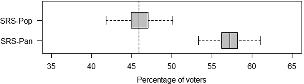
Random samples from the population and from the panel.

The distribution of the sample mean for random samples from the population is displayed in the upper part of the graph (SRS-Pop). The box plot shows there is a symmetrical distribution around the value to be estimated (45.9%). This indicates an unbiased estimator. This is the ideal situation, which will be used as a benchmark for other estimation techniques. The distribution of the sample mean for samples from the panel is displayed in the lower part of the graph (SRS-Pan). The whole distribution has shifted to the right. The values of the estimator are systematically too high. Their average is 57.2%. This indicates a biased estimator. This is caused by the fact that the panel is not representative for the population.

Now, the effect of sample matching is explored. Each sample from the frame is matched to the panel and the sample average is computed for the linked persons. Three situations are considered. In the first one, only the auxiliary variable age (in three categories) is used for matching. In the second one, only the variable education (in two categories) is used. And in the third one, both age and educated are used for matching.

The set of matching variables only takes a limited number of values. So, it will not be a problem to find matching persons in the panel. In case of more candidates, a random person is taken. The distributions of the resulting estimators are shown in Figure 2.

OPEN IN VIEWER

Figure 2.

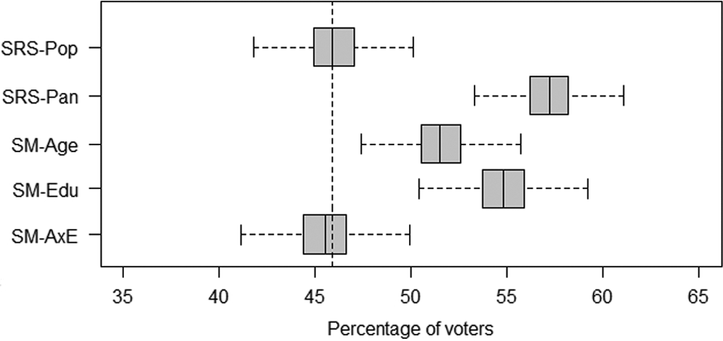
The distribution of matched sample.

The distribution for the matched sample estimator based on just the variable age is denoted by SM-Age. The estimator is biased, but the bias is smaller than that of the SRS-Pan. Still, all possible values of the estimator are significantly too high. The expected value of the estimator is 51.5%, which means a bias of 51.5% – 45.9% = 5.6%.

The distribution for the matched sample estimator based on just the variable education is denoted by SM-Edu. This estimator performs even worse than that of SM-Age. The bias of the SM-Edu estimator is smaller than that of samples from the panel, but it is still very large. The expected value of the SM-Edu estimator is equal to 54.8%, which comes down to a bias of 54.8% − 45.9% = 8.9%.

The bias vanishes when both variables age and education are used for sample matching. The distribution of the resulting estimator is denoted by SM-AxE. It is not surprising that the bias vanishes, because all variables used for sample matching also explain participation behavior for the panel. If, for example, just the variable age would have been used for matching, there are still differences between young people inside the panel and outside the panel. High educated young people are overrepresented in the panel. Therefore, their voting probability is higher. If both variables age and education are used for sample matching, there are no differences any more between members of groups inside and outside the panel. They have the same voting probabilities.

The results of the simulations are summarized in Table 3. The conclusion can be drawn that sample matching will not always remove the bias of estimators. This depends on the set of variables that is used for matching the sampling frame and the panel. Sample matching is only successful if all explanatory variables are used that are required to explain the participation behavior of the panel members. If not all relevant variables are used, only part of the bias will be removed.

OPEN IN VIEWER

Table 3.

Summary of the Simulation Results (10,000 Simulations of Samples of Size 1,000).

Estimation	Expected value	Bias	SD
Simple random sample from the population	45.93	−0.01	1.57
Simple random sample from the panel	57.21	11.27	1.43
Sample matching using age	51.52	5.58	1.55
Sample matching using education	54.79	8.85	1.58
Sample matching using age and education	45.50	−0.44	1.58

Stratified Sampling

The matched sample estimator as defined by expression (18) can also be written as

y ˉ S M = ∑ h = 1 L n h n y ˉ h ,

22

where y ˉ h is the mean of the n_h observations in group h. The quantity n_h /n is an unbiased estimator of the quantity N_h /N. Therefore, a different estimator can be obtained by replacing n_h /n by N_h /N in expression (22). This results in

y ˉ S T = ∑ h = 1 L N h N y ˉ h .

23

This is the estimator that would have been obtained for stratified sampling from the frame with proportional allocation, that is, the sample sizes n_h in the strata are proportional to the sizes N_h of the strata in the population. In practice, this would mean using the sampling frame to determine the stratum sizes and then selecting a stratified sample from the panel.

To explore the behavior of estimator (23), the simulation study in the fourth section was continued. Stratified samples of size 1,000 were drawn from the panel. This was repeated 10,000 times. The resulting distributions of the estimators are displayed by means of box plots. Figure 3 compares the distributions of the three matched sample estimators with the corresponding stratification estimators.

OPEN IN VIEWER

Figure 3.

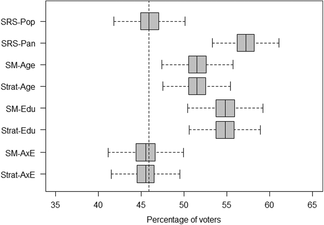
The distribution of stratification estimators.

The performance of the stratification estimator with respect to bias reduction is the same as that of the matched sample estimator. The bias reduction of the sample matching using the variable age (denoted by SM-Age) is of the same magnitude as the bias reduction of stratification by age (denoted by Strat-Age). Similarly, the bias reduction of SM-Edu is the same as that of Strat-Edu. Finally, both SM-AxE and Strat-AxE are capable of removing the bias completely.

The results of the simulation are summarized numerically in Table 4. The table confirms the conclusions based on the graph: The matched sample estimator and the stratification estimator have the same behavior with respect to reducing the bias.

OPEN IN VIEWER

Table 4.

Comparing Sample Matching With Stratification (10,000 Simulations of Samples of Size 1,000).

Estimation	Expected value	Bias	SD
Sample matching using age	51.52	5.58	1.55
Stratification using age	51.51	5.57	1.50
Sample matching using education	54.79	8.85	1.58
Stratification using education	54.79	8.85	1.57
Sample matching using age and education	45.50	−0.44	1.58
Stratification using age and education	45.51	−0.43	1.45

Note that the stratification estimators have slightly smaller standard deviations. The reason is that the number of observations per group is fixed. In contrast, the number of observations per group for the matched sample estimators are the result of selecting a random sample from the sampling frame. This introduces an extra source of variation.

Post-Stratification Estimation

One of the obvious approaches to obtain less biased estimators from a self-selection panel would be to draw a simple random sample from the panel, followed by a bias reduction attempt by means of post-stratification. So the panel itself is used as a sampling frame and the original sampling frame serves to compute the population distribution of weighting variables. The expression for the post-stratification estimator becomes

y ˉ P S = ∑ h = 1 L N h N y ˉ h = ∑ h = 1 L N h N 1 n h ∑ i = 1 n h y h i ,

24

where the values y_hi are obtained by means of a simple random sample from the panel. Expression (24) resembles expression (23). The difference is, however, that in the case of stratification, a stratified sample is selected from the panel; and in case of post-stratification, a simple random sample is selected from the panel.

The panel is not representative for the population. Since the sample for post-stratification is selected from this panel, one can expect serious representativity problems. This was already shown in Figure 1. Therefore, weighting adjustment is badly needed in an attempt to reduce the bias of estimators.

To explore the behavior of estimator (24), the simulation study was continued. Samples of size 1,000 were drawn from the panel. This was repeated 10,000 times. The resulting distributions of the post-stratification estimators are displayed by means of box plots. Figure 4 compares the distributions of various matched sample estimators, with the corresponding stratification and post-stratification estimators.

OPEN IN VIEWER

Figure 4.

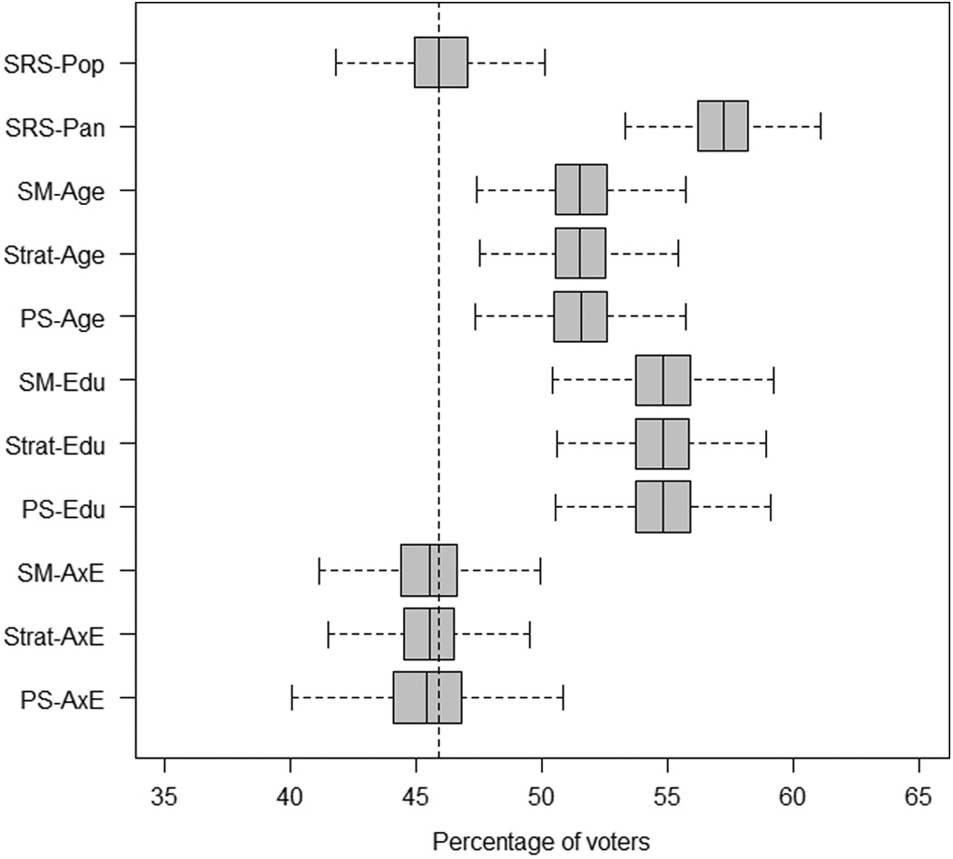
The distribution of matched sample estimators, stratification estimators, and post-stratification estimators.

The performance of the post-stratification estimator with respect to bias reduction is the same as that of the stratification estimator and the matched sample estimator. The magnitude of the bias reduction does not depend on the type of estimator but on the variables used. There is a limited bias reduction if only the variable education is used. There is more bias reduction for the variable age. And the bias is completely removed when both variables are used.

Note that the variance of the post-stratification estimator for age by education (denoted by PS-AxE) is clearly larger than that of the corresponding matched sample estimator (MS-AxE) and stratification estimator (Strat-AxE). The extra variation is the between strata component of the sampling variability.

The results of all simulations are summarized in Table 5. It is clear that the properties of the three types of estimators are more or less the same in this simulation study. There is no reason to think that it would be different in other situations.

OPEN IN VIEWER

Table 5.

Comparing Sample Matching With Stratification and Post-Stratification (10,000 Simulations of Samples of Size 1,000).

Estimation	Expected value	Bias	SD
Sample matching using age	51.52	5.58	1.55
Stratification using age	51.51	5.57	1.50
Post-stratification using age	51.53	5.59	1.57
Sample matching using education	54.79	8.85	1.58
Stratification using education	54.79	8.85	1.57
Post-stratification using education	54.81	8.87	1.61
Sample matching using age and education	45.50	−0.44	1.58
Stratification using age and education	45.51	−0.43	1.45
Post-stratification using age and education	45.46	−0.48	2.00

The conclusion can be that if a panel (possibly constructed by means of self-selection) is available and the population distributions of the set of relevant auxiliary variables, one could simply apply post-stratification. Sample matching would not produce better estimates in terms of bias. Stratified sampling results in somewhat smaller standard errors than sample matching.

It is stressed once more that the bias will only be removed completely if all auxiliary variables are available that are needed to completely explain participation behavior. In practice, this will often not be the case. Then, the bias will only be reduced somewhat, but not removed completely. So, auxiliary variables play an important role.