Using Multilevel Models to Explore Predictors of High School Students’ Nonresponse in Experience Sampling Method (ESM) Studies

Abstract

This study uses multilevel generalized linear models to examine predictors of high school students’ nonresponse when using the experience sampling method (ESM), a form of momentary data collection that captures participants’ situational thoughts, feelings, and emotions. Because ESM approaches often seek to generalize and compare participants’ emotional states across days and times, it is important to understand how and when participants may miss response opportunities, and further to explore how this response bias may limit generalizability of findings. Results from this study, conducted in three mid-Michigan high schools in 2013–2014 with a sample of 141 students, indicate that time of day and day of week are significantly related to a given participant’s odds of nonresponse. Specifically, ESM “prompts” occurring after school and over the weekend had much higher odds of being missed by participants, even after controlling for other covariates such as race/ethnicity, gender, and person-level emotional trends. These findings demonstrate that day and time contextual factors are significantly related to odds of nonresponse, and researchers using these approaches to compare widely different time contexts should be mindful of possible generalizability concerns.

Keywords

experience sampling method (ESM)generalizability multilevel modeling nonresponse

Research designs using the experience sampling method (ESM)—a form of time diary data collection (Hektner, Schmidt, & Csikszentmihalyi, 2007; Mehl & Conner, 2011)—have grown dramatically in popularity over the last decade, particularly in education and the social sciences (Zirkel, Garcia, & Murphy, 2015). The flexibility of the method, as well as its ability to capture in-the-moment data from participants across a variety of contexts, offer unique advantages to researchers seeking to understand phenomena embedded in daily life and social interactions. ESM approaches frequently provide rich subsamples of daily activity but also present unique challenges in the areas of nonresponse and missing data (Jeong, 2005).

While the general psychometric properties of longitudinal data have been increasingly well established (Singer & Willett, 2003), less is known about the specific statistical properties of ESM designs (an intensive longitudinal method, see Bolger & Laurenceau, 2013) which usually compress longitudinal data collection into a period of days or weeks. Within this brief time period, participants can often complete the short ESM surveys 40 or 50 times. As a result, researchers can often collect rich data on participants’ thoughts, feelings, and actions in multiple spatial and social contexts over the course of a week. Nevertheless, participants inevitably miss scheduled prompts, and over the course of a week, these patterns of missed prompts need to be closely examined in order to make sound generalizations about a given sample and population.

Related Literature

Overview of Experience Sampling

Experience sampling research is a rapidly developing research methodology that aims to capture in-the-moment responses from participants over the course of their daily life. Since its initial development in psychology (e.g., Csikszentmihalyi & Larson, 1987; Hormuth, 1986), experience sampling has been applied to a wide variety of research fields spanning education, psychology, sociology, economics, and medicine (Hektner et al., 2007). Across these fields, the approach is alternately referred to as ecological momentary analysis (Stone & Shiffman, 1994; Wilhelm, Perrez, & Pawlik, 2011) and event sampling (Reis & Gable, 2000).

A typical ESM study usually involves developing a short questionnaire that captures a phenomenon of interest, such as different types of task behaviors (What are you doing?), affective states (How do you feel?), or measures of social proximity (Who are you with?). Questionnaires are typically brief, completed in 1–2 min or less, and can contain a variety of Likert-type question scales and sometimes short open response questions. Participants are then prompted (either randomly or at fixed time intervals) to stop and respond to the questionnaire multiple times throughout a day, typically 5–10 times per day over the course of a week or more.

The process of data collection in ESM studies has historically been a logistical challenge (Hektner et al., 2007). Initially, participants were often given preprogrammed wristwatches or pagers and paper versions of the ESM questionnaire which they would fill out when prompted. Over the past several decades, the proliferation of relatively inexpensive handheld devices, such as Palm Pilots and other PDAs, led to more digital collection of ESM data (Burgin, Silvia, Eddington, & Kwapil, 2012). Most recently, cell phones have emerged as a powerful alternative, offering more flexibility and customization via the use of mobile applications and short message service text messaging (Hofmann & Patel, 2015; Thomas & Azmitia, 2016).

ESMs offer several advantages to researchers interested in studying daily life experiences. First, ESM approaches allow for rich, in-the-moment data collection related to participants’ affective states and daily behaviors (Barrett & Barrett, 2001). Repeated, embedded data collection offers unique perspectives on individual behavior that may not be captured from other types of surveys that are administered at only one time point. In addition, ESM can be adapted to suit a wide variety of research questions and paradigms, as evidenced by its growth in numerous scientific fields (Zirkel et al., 2015).

ESM approaches also have several key limitations. First, ESM surveys, which are given multiple times per day, present a unique burden on participants compared to single time point surveys. In addition, ESM designs can be complicated to implement and require significant time and resources for working with cell phones, PDAs, and so on to ensure the collection process runs smoothly. Finally, experience sampling, like all survey-based data collection methods, is vulnerable to nonresponse, when participants are unable (or unwilling) to respond to a prompt and complete a questionnaire. Issues of nonresponse are well developed in the field of survey research and are becoming more developed in the specific context of experience sampling. Both are briefly described below.

Nonresponse in Related Survey Research

While the body of research on nonresponse is less developed in the ESM context, the issue of nonresponse and potential bias resulting from nonresponse has been much more developed in other subfields of survey research and design. For example, researchers interested in time use have long considered the potential impacts of nonresponse on time use estimates. Mulligan, Schneider, and Wolfe (2005) analyzed ESM data from the Alfred P. Sloan Study of Youth and Social Development and compared respondents’ estimates of time spent working to similar estimates obtained using a time diary approach in the American Time Use Survey and the National Educational Longitudinal Study of 1988 and found that differential rates of nonresponse by gender and time of day in the ESM sample significantly impacted population-level estimates of time use. However, this impact could be corrected for in several ways, such as using weighting techniques on observed data or multiple imputation to adjust for missingness (Diggle, Heagerty, Liang, & Zeger, 2002; Hedeker & Gibbons, 2006).

In addition to time use research, nonresponse bias is also a significant concern for researchers designing and implementing large-scale household surveys (Bethlehem, Cobben, & Schouten, 2011; Kreuter, Couper, & Lyberg, 2010; Wagner, 2010). Here, researchers might build a probability sample by calling households and asking a series of survey questions. As rates of refusal or nonresponse for these types of calls have increased over the last 15 years (Couper, 2005; Groves, 2006), survey statisticians have become much more interested in how factors like time of day and day of week might influence rates of participant nonresponse or compliance, and further, how nonresponse bias might impact the generalizability of even large-scale household surveys.

Nonresponse in ESM Research

To date, limited research has been conducted on the predictors of nonresponse in ESM studies; however, results of this work suggest that demographic characteristics, such as gender, and contextual characteristics, such as time of day and day of week, may significantly impact the odds of nonresponse. For example, Silvia, Kwapil, Eddington, and Brown (2013) examined dispositional and situational predictors of nonresponse in a sample of 450 college students and found that males were significantly more likely than females to miss prompts. In addition, missed prompts were significantly more likely to occur later in the day (after 4 p.m.) and later in the study week. The researchers attribute this effect to increased survey fatigue of participants, who tire of responding at the end of each day and, eventually, during the middle and end of the entire study period.

A second study by Messiah, Grondin, and Encrenaz (2011) examined factors influencing nonresponse in a single sample of 224 French university students and again found that males were significantly more prone to nonresponse. Further, participants in this study had higher odds of nonresponse for prompts occurring in the middle of the week (on Tuesday, Wednesday, or Thursday) and first thing in the morning (from 8 to 11 a.m.). A third study by Courvoisier, Eid, and Lischetzke (2012) analyzed the factors influencing nonresponse in a sample of 318 university students in Switzerland and found that the odds of nonresponse were lowest between 5 and 7 p.m. and highest between 9 and 11 a.m. The researchers also found a slight increase in the odds of nonresponse as the study progressed, particularly between Day 4 and Day 7, the last day of the study.

Missing Data and Generalizability

As suggested, nonresponse poses challenges to survey-based research by potentially biasing estimates. In an ESM context, each missed prompt represents a vector of missed data points, as participants are typically asked to respond to a series of survey questions at each time point. In general, quantitative researchers have developed different classifications for types of missing data (Allison, 2002; Rubin, 1976); these include missing completely at random (MCAR), missing at random (MAR), and not missing at random (NMAR). Each classification is associated with a series of assumptions about the underlying data. For example, missing data are considered to be MCAR if the likelihood of an item being missed is unrelated to any other observed variable as well as unrelated to any unobserved confounders.

Data are assumed to be MAR, a less demanding assumption, if, after controlling for auxiliary variables, such as time, day, or gender, likelihood of missingness is not related to the outcome in question. In other words, if within each stratum, or level, of a particular control variable, the probability of a participant missing a prompt is randomly distributed, then data can be assumed to be (conditionally) MAR.

Figures 1– 3 demonstrate graphically what MCAR and MAR data may look like in the ESM context. All three figures display a 7 by 8 grid representing the total possible sample of prompts one person may receive throughout the course of a week in an ESM study (typically participants receive about 8 prompts per day, over the course of 7 days, which total to 56 possible prompts). Each cell in the grid represents one response; if the cell is clear, that particular prompt was responded to, if the cell is dark gray, that particular prompt was missed.

Figure 1.

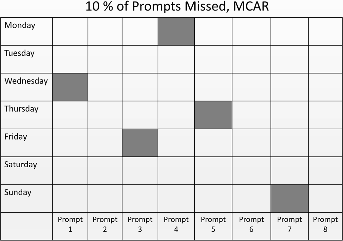
Graphic representation of missed prompts, 10% missed, missing completely at random (MCAR) selection process. Dark gray squares indicate a missed prompt.

Figure 2.

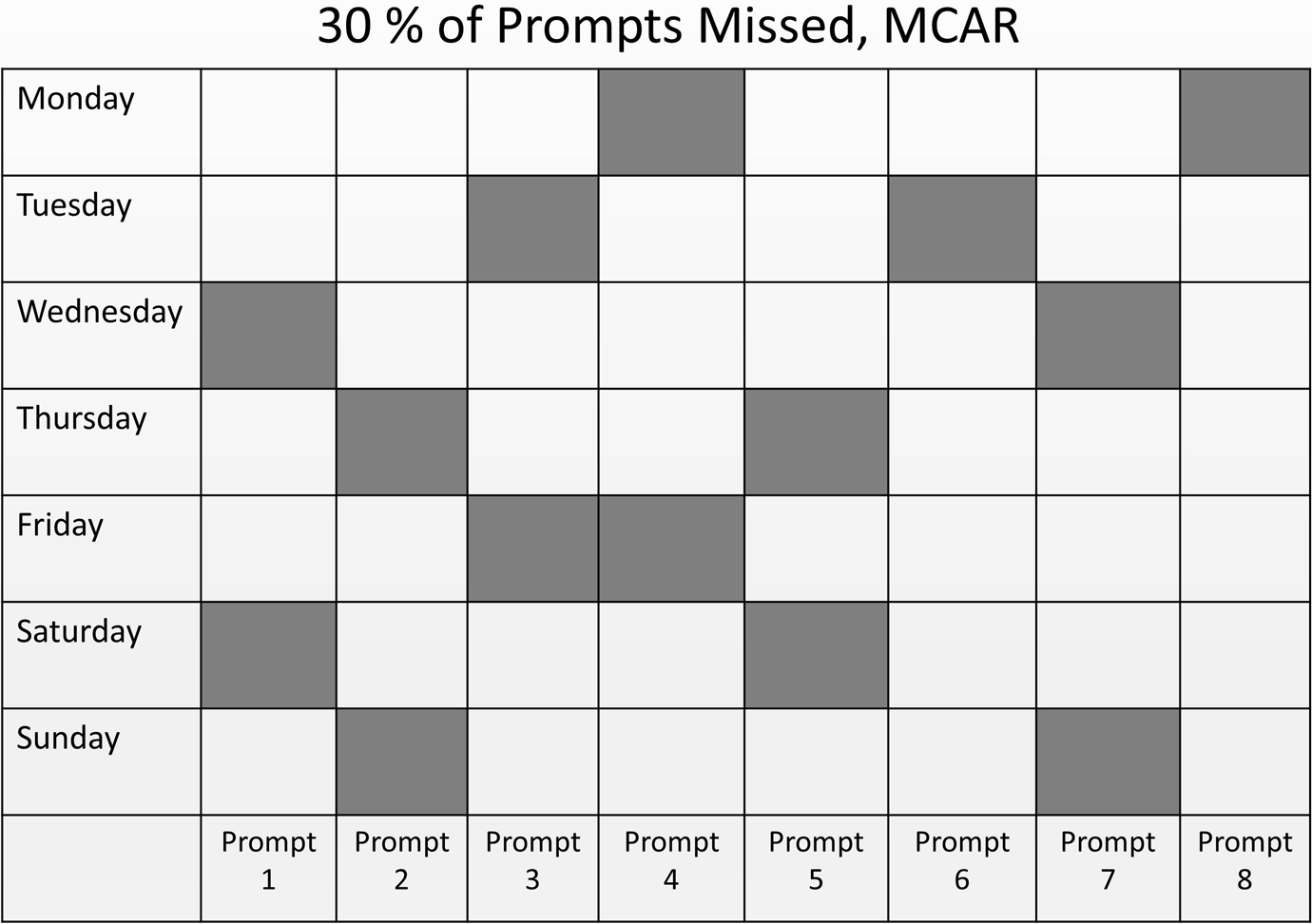
Graphic representation of missed prompts, 30% missed, missing completely at random (MCAR) selection process. Dark gray squares indicate a missed prompt.

Figure 3.

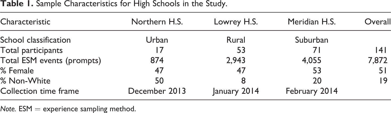
Graphic representation of missed prompts, 30% missed, missing at random (MAR) selection process. Dark gray squares indicate a missed prompt.

Figure 1 illustrates a set of responses that would likely satisfy the MCAR assumptions—overall, only 10% of prompts are missing, and the missingness appears to be occurring randomly across days and times (prompts). Likewise, Figure 2 reflects a largely MCAR process—although in this case, rates of missingness are much higher, at 30%. Here, despite the higher overall presence of missed prompts, the probability of missingness does not appear to vary across days or times.

Figure 3 again displays a set of responses with 30% of prompts missed, however in this case the prompts are not MCAR. Prompts occurring later in the day and on the weekend appear to have much higher probabilities of nonresponse. This example does not satisfy the assumptions of MCAR, given the impact of day and time on response. MAR assumptions, however, could still be met by applying appropriate statistical controls to mitigate the differential probability of nonresponse by day and time (Allison, 2002). However, any outcome used in analysis would need to be carefully examined for its relationship to missingness, both before and after controlling for day and time. In the event that conditioning on day, time, and other covariates is unable to account for differential response, ESM data may be considered NMAR, a condition that necessitates far more complex statistical approaches to achieve generalizability (Allison, 2002).

The figures above illustrate the complexity of understanding patterns of missing data and responses in ESM research. This study applies multilevel modeling, which can simultaneously examine patterns of missingness due to prompt-level, day-level, and person-level characteristics, to examine a sample of 7,872 prompts collected from 141 students in three high schools in mid-Michigan in 2013–2014. The relevant research questions are below.

Research Questions

How are factors of time and daily context associated with participants’ odds of missing an ESM response?

How are person-level demographic factors (e.g., gender, race, school) associated with participants’ odds of missing an ESM response?

How are in-the-moment and person-averaged measures of student emotional states associated with participants’ odds of missing an ESM response, after controlling for other relevant time- and person-level predictors?

Method

Data Collection

This study made use of a new smartphone application (app), Paco (www.pacoapp.com), developed by Robert Evans, which is open source and specifically designed for the ESM. The ESM instrument was transferred to smartphones using a web-based program that also uploads, stores, and protects participant data prior to analysis.

For a week in winter 2013 and early spring 2014, students in the study were given smartphones with Paco installed. Each time students were signaled during the day, they were asked to respond to a set of identical items within a 15-min window. On average, it takes about 60 s to complete the items. All students received training on how to use Paco prior to data collection, and their teachers also were briefed on study procedures. Students were asked to provide assent for the study; 2 students out of the sample of 143 declined to participate. All data were stored on a secure data server and de-identified to maintain confidentiality.

Each day over a week all students received 8 prompts on their smartphones, which gave them 56 total response opportunities. The preprogrammed randomized prompt schedule ran from 8 a.m. to 8 p.m. daily and guaranteed a minimum of four prompts in the morning and an additional four prompts between 1 p.m. and 8 p.m. Prompts were scheduled to be slightly more frequent in the morning in an effort to capture additional prompts in students’ science classes, which occurred before noon.

Sample

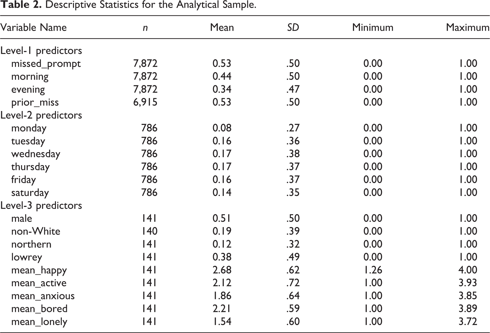
The sample includes 141 students (62 males and 79 females) in three secondary schools in the mid-Michigan area. According to U.S. Census classifications, one school is urban, one is suburban, and one is rural. The schools and teachers were selected on a voluntary basis and all students in each science class were invited to participate. About 19% of students in the sample self-identified as non-White. Table 1 presents descriptive statistics and characteristics for the three high schools in the study: Meridian High School, Northern High School, and Lowrey High School. School names used here are pseudonyms.

Table 1.

Sample Characteristics for High Schools in the Study.

Characteristic	Northern H.S.	Lowrey H.S.	Meridian H.S.	Overall
School classification	Urban	Rural	Suburban
Total participants	17	53	71	141
Total ESM events (prompts)	874	2,943	4,055	7,872
% Female	47	47	53	51
% Non-White	50	8	20	19
Collection time frame	December 2013	January 2014	February 2014

Note. ESM = experience sampling method.

Measures

Table 2 presents descriptive statistics for the variables used in this study. Below, the measurement and operationalization of each variable are described. Variables are separated into two conceptual categories: (1) time-variant predictors, which vary within student and across time and (2) time-invariant predictors, which only vary between students. These distinctions will be further defined by the statistical approach outlined in the analysis section.

Table 2.

Descriptive Statistics for the Analytical Sample.

Variable Name	n	Mean	SD	Minimum	Maximum
Level-1 predictors
missed_prompt	7,872	0.53	.50	0.00	1.00
morning	7,872	0.44	.50	0.00	1.00
evening	7,872	0.34	.47	0.00	1.00
prior_miss	6,915	0.53	.50	0.00	1.00
Level-2 predictors
monday	786	0.08	.27	0.00	1.00
tuesday	786	0.16	.36	0.00	1.00
wednesday	786	0.17	.38	0.00	1.00
thursday	786	0.17	.37	0.00	1.00
friday	786	0.16	.37	0.00	1.00
saturday	786	0.14	.35	0.00	1.00
Level-3 predictors
male	141	0.51	.50	0.00	1.00
non-White	140	0.19	.39	0.00	1.00
northern	141	0.12	.32	0.00	1.00
lowrey	141	0.38	.49	0.00	1.00
mean_happy	141	2.68	.62	1.26	4.00
mean_active	141	2.12	.72	1.00	3.93
mean_anxious	141	1.86	.64	1.00	3.85
mean_bored	141	2.21	.59	1.00	3.89
mean_lonely	141	1.54	.60	1.00	3.72

Study outcome: Missed prompt

The outcome in this study, missed_prompt, is measured as a 0 if a given prompt was responded to and 1 if the prompt was not responded to within the 15-min window specified by the study design. The mean of this measure, 0.53, indicates that about 53% of scheduled prompts in the study were missed. The predictors described below are included to help identify the factors that are most associated with the probability of missing a prompt.

Level-1 predictors

Three predictors were used to identify effects of day and time on missed prompts. Morning is a dichotomous measure that is equal to 1 when a prompt occurred before noon on a given day and 0 otherwise. This measure is especially useful in this case because students in the sample all attended science class in the morning. Since science teaching and learning were the driving motivation behind the initial research (see Schneider et al., 2016), and science teachers were active participants and collaborators in the work, one might expect that students would miss fewer prompts in the morning.

A second time predictor, evening, is a dichotomous measure equal to 1 when a prompt occurs after 4 pm on a given day and 0 otherwise. This variable allows for a useful distinction by contrasting students’ behaviors during and after school. Since these two contexts are quite different, one would expect that patterns of missed prompts may vary accordingly. In addition to predictors of time, a lagged measure of the dependent variable, prior_miss, was also used in the final statistical model. In this case, only a students’ response in the immediately preceding time unit was used. Lags beyond one unit were not used as the gap in time between the initial response and the missed prompt would be quite significant (i.e., many hours or even a full day).

Level-2 predictors

At Level 2, a series of six dichotomous predictors were included. These corresponded to days of the week in which a prompt was sent. This resulted in six unique predictors, Monday–Saturday, and the reference category, Sunday, which was left out.

Level-3 predictors

In addition to time-variant predictors, several time-invariant predictors were used to examine person-level associations with the probability of a missed prompt. These include dichotomous predictors of gender (male), race/ethnicity (non-White), and school assignment (northern and lowrey). Further, average levels of students’ emotional states were included (mean_happy, mean_active, mean_anxious, mean_bored, and mean_lonely). These values represent the average response for each student over the course of the study and were included to serve as proxies for person-level differences in average emotional levels. Emotional states were measured on a scale from 1 to 4, with higher values corresponding to stronger feelings (see Appendix for the complete ESM instrument).

Analyses

The ESM data are analyzed using three-level hierarchical generalized linear models (HGLMs; Rabe-Hesketh & Skrondal, 2008; Raudenbush & Bryk, 2002), which include in-the-moment student responses and contextual measures (e.g., time) at Level 1, day of week-specific predictors at Level 2, and static student characteristics (e.g., gender, race/ethnicity, and average emotional states) at Level 3. This particular three-level approach has been adopted to more accurately estimate time, day, and person-level influences on the odds of nonresponse (Hawkley, Preacher, & Cacioppo, 2007; Walls, Jung, & Schwartz, 2006). To estimate the association of time and day factors with person-level characteristics on the odds of a missed prompt, the following three-level random-intercept logistic regression was used, specified for time (instance) t nested within day i and person j:

Equation 1: The association of prompt-level, day-level, and person-level predictors with the likelihood of nonresponse.

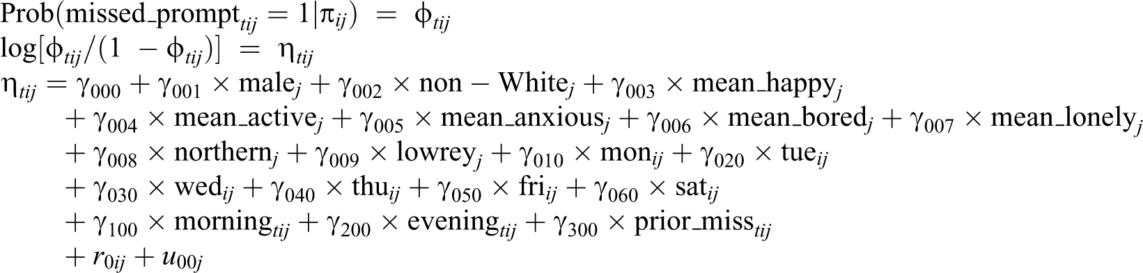
\begin{array}{l} {Prob(missed_prompt}_{t i j} = 1 | π_{i j}) = φ_{t i j} \\ log [φ_{t i j} / (1 - φ_{t i j})] = η_{t i j} \\ η_{t i j} = γ_{000} + γ_{001} \times {male}_{j} + γ_{002} \times {non-White}_{j} + γ_{003} \times {mean_happy}_{j} \\ + γ_{004} \times {mean_active}_{j} + γ_{005} \times {mean_anxious}_{j} + γ_{006} \times {mean_bored}_{j} + γ_{007} \times {mean_lonely}_{j} \\ + γ_{008} \times {northern}_{j} + γ_{009} \times {lowrey}_{j} + γ_{010} \times {mon}_{i j} + γ_{020} \times {tue}_{i j} \\ + γ_{030} \times {wed}_{i j} + γ_{040} \times {thu}_{i j} + γ_{050} \times {fri}_{i j} + γ_{060} \times {sat}_{i j} \\ + γ_{100} \times {morning}_{t i j} + γ_{200} \times {evening}_{t i j} + γ_{300} \times {prior_miss}_{t i j} \\ + r_{0 i j} + u_{00 j} \end{array}

Level-1 variance of random effect = 1 / [φ_{t i} (1 - φ_{t i})]

Parameterization of Level 2 and Level 3 random effects:

r_{0 i j} \sim N (0, τ_{00}^{(2)}),

u_{00 j} \sim N (0, τ_{00}^{(3)}) .

In order to better understand how groups of predictors relate to one another, the analysis was conducted following a typical model building approach (Hox, 2010) that includes four separate models. Model 1 includes only Level 1 and Level 2 predictors of time and day. Model 2 adds on Level 3 predictors of gender, race/ethnicity, and school assignment. Model 3 includes person-level averages of emotional states, while Model 4, the full model, incorporates all the covariates discussed above plus the lagged dependent variable. The advantage of this approach is that it allows for examination of how estimates of key covariates, such as time, place, and gender, are influenced by the introduction of additional predictors.

Main results presented below come from Equation 1, applying conditional (or unit-specific) assumptions. Analysis was performed using HLM (version 7) (Raudenbush, Bryk, & Congdon, 2011), which uses maximum likelihood estimation with adaptive Gauss-Hermite quadrature. This means that log odds (η _tij ) should be interpreted as conditional on all covariates as well as the Level-2 (r_0ij ) and Level-3 (u_00j ) random effects. This study’s focus on within-person processes suggests that a conditional model, as opposed to a marginal, or population-average approach, is the best choice (Raudenbush & Bryk, 2002). However, population-averaged estimates are available from the author. This estimation procedure employs a generalized estimation equation to average coefficient estimates across all Level-2 and Level-3 distributions (Rabe-Hesketh & Skrondal, 2008). In this case, however, estimates from the unit-specific and population-averaged approaches did not appear to differ significantly in terms of magnitude or significance.

Calculating Predicted Probabilities

Given the complexity of interpreting log-odds coefficients produced by HGLMs, often it is useful to convert the estimated log odds (η _tij ) into predicted probabilities. This was accomplished using the -margins- command in Stata (StataCorp, 2013), after fitting an identical model to the one described in Equation 1. These probabilities and their standard errors can then be used to compare relative odds of missed prompts across the entire week.

Missing Data

Missing data is often an important consideration in ESM research, which can be susceptible to higher rates of missingness (a key motivation of this study). In this case, however, there was no missing data in the sample for Models 1–3. This is largely due to the construction of the analysis, which relies on measures of dates and times that are automatically recorded by the ESM software as well as person-level measures that can readily be obtained from school administrative data. Therefore, all scheduled prompts are included in the current sample. Model 4, which includes a lagged measure of the dependent variable (a missed prompt), does introduce more missing data—in this case, the first prompt given each day is dropped from the sample, since there is no corresponding prior state. This reduced the overall sample size by about 1,000 prompts (out of 7,872 total).

One additional possibility exists for missing data; if cell phones are turned off, ESM prompts do not occur, and are likewise not registered as being missed. So, broken or powered-down phones may not record prompts properly. This is a somewhat difficult phenomenon to quantify, but one approach is to estimate how many prompts should have occurred over the course of the week, and then compare that number to the number of prompts that actually occurred. In the case of this sample, with 141 total participants, the phones should have been prompted a total of 7,896 times (the product of 141 and 56, the number of weekly prompts). In actuality, the phones in this sample were prompted a total of 7,872 times, which is within 0.4% of the expected prompt total. Ideally, the expected and actual prompt totals would be identical, but some small variation is expected due to the factors discussed above (and other random errors). In sum, there appears to be little evidence that participants turned their phones off during the day and missed prompts, which suggests that the sample collected is a reasonably accurate snapshot of missed and responded prompts.

Results

Table 3 below presents unit-specific results sequentially for all four statistical models. Results are summarized by model. Coefficients presented have been translated to odds ratios (ORs) by exponentiating the log-odds (η _tij ) coefficients (OR = exp(η _tij )). Thus, ORs greater than 1 suggest that particular times, states, and so on are associated with increased odds of missing prompts, and likewise, ORs less than 1 suggest that a predictor is associated with a decrease in odds of missing prompts.

Table 3.

Fixed Effects Estimates (Top) and Variance–Covariance Estimates (Bottom) for Models of the Predictors of a Missed Signal.

	(1) Time and Day Only		(2) Plus Demographics		(3) Plus Average States		(4) Plus Lag Effect
Variables	OR	95% CI	OR	95% CI	OR	95% CI	OR	95% CI
Fixed effects
Intercept	3.03***	[2.24, 4.10]	3.29***	[2.20, 4.93]	0.61	[0.15, 2.55]	0.43	[0.13, 1.43]
Level 1 (signal)
morning	0.58***	[0.52, 0.67]	0.58***	[0.52, 0.67]	0.58***	[0.52, 0.67]	0.63***	[0.55, 0.75]
evening	1.36***	[1.17, 1.57]	1.36***	[1.15, 1.51]	1.36***	[1.15, 1.51]	1.25**	[1.02, 1.49]
prior_miss							2.33***	[1.89, 2.82]
Level 2 (day)
monday	0.24***	[0.17, 0.34]	0.24***	[0.17, 0.34]	0.23***	[0.16, 0.34]	0.36***	[0.26, 0.50]
tuesday	0.25***	[0.19, 0.34]	0.25***	[0.18, 0.34]	0.25***	[0.18, 0.34]	0.35***	[0.27, 0.45]
wednesday	0.40***	[0.30, 0.53]	0.40***	[0.30, 0.53]	0.40***	[0.30, 0.53]	0.51***	[0.40, 0.66]
thursday	0.47***	[0.35, 0.63]	0.47***	[0.35, 0.64]	0.47***	[0.35, 0.63]	0.56***	[0.44, 0.72]
friday	0.44***	[0.33, 0.60]	0.45***	[0.33, 0.60]	0.44***	[0.33, 0.60]	0.51***	[0.40, 0.66]
saturday	1.00	[0.74, 1.35]	1.00	[0.74, 1.35]	1.00	[0.74, 1.35]	1.03	[0.80, 1.33]
Level 3 (person)
male			0.79	[0.55, 1.14]	0.85	[0.59, 1.24]	0.89	[0.65, 1.21]
non-White			1.04	[0.63, 1.72]	1.02	[0.62, 1.68]	0.99	[0.65, 1.49]
northern			0.67	[0.37, 1.24]	0.66	[0.36, 1.19]	0.68	[0.42, 1.12]
lowrey			1.21	[0.82, 1.81]	1.31	[0.87, 1.96]	1.21	[0.86, 1.69]
mean_happy					1.37	[0.93, 2.01]	1.33†	[0.97, 1.84]
mean_active					0.88	[0.64, 1.22]	0.86	[0.66, 1.12]
mean_anxious					1.04	[0.75, 1.44]	1.03	[0.79, 1.35]
mean_bored					1.65**	[1.14, 2.38]	1.48*	[1.09, 2.01]
mean_lonely					0.92	[0.64, 1.30]	0.96	[0.72, 1.28]
Random parameters
Level-2 variance, r ₀	0.41***		0.41***		0.41***		0.14***
Level-3 variance, u ₀₀	0.82***		0.78***		0.73***		0.49***
Deviance	22,596.17		22,590.99		22,582.40		19,705.82
Number of parameters	11		15		20		21
Observations	7,872		7,872		7,872		6,915
Number of students	141		140		140		140

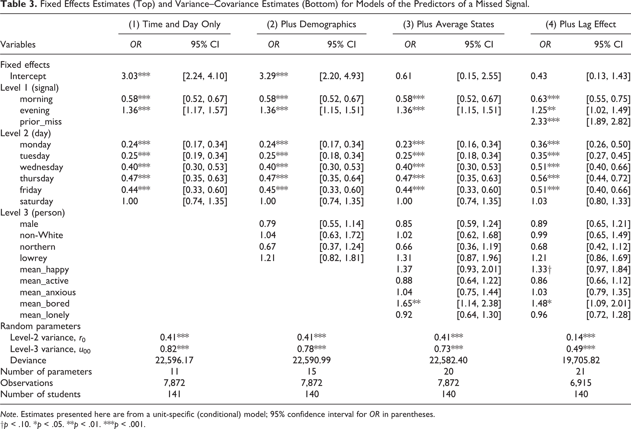
Note. Estimates presented here are from a unit-specific (conditional) model; 95% confidence interval for OR in parentheses.

†p < .10. *p < .05. **p < .01. ***p < .001.

Model 1: Time and Day Predictors

Fitting an HGLM with just prompt-Leve-l (Level-1) and day-level (Level-2) covariates (see Table 3, column 1), both Level-1 predictors were found to be significantly associated with the likelihood of nonresponse, after controlling for other covariates and the Levels-2 and 3 random effects. Prompts occurring in the morning (OR = 0.58, p < .001) had about half the odds of being missed compared to prompts in the afternoon. Prompts occurring in the evening (OR = 1.36, p < .001) were associated with significantly higher odds of nonresponse. In this case, prompts delivered in the evening were about 1.3 times more likely to be missed than prompts occurring in the afternoon. At Level 2, prompts delivered on a weekday were much more likely to receive a response than a prompt delivered on Sunday. ORs ranged from 0.24 (p < .001) on Monday to 0.47 (p < .001) on Thursday. Prompts delivered on a Saturday, however, did not differ significantly in terms of the odds of nonresponse (OR = 1.00, p > .10) relative to prompts delivered on a Sunday.

Model 2: Student Demographics and School Assignment

Model 2 included the same Level-1 and Level-2 predictors discussed above along with several Level-3 (person-level) predictors (see Table 3, column 2). Estimates of Level-1 and Level-2 predictors did not change in terms of magnitude or significance. At Level 3, no person-level predictors were significantly associated with the likelihood of nonresponse, after adjusting for other covariates and the Level-2 and Level-3 random effects. Estimates of gender, race/ethnicity, and school assignment were not significant.

Model 3: Person-Level Emotional States

Model 3 (see Table 3, column 3) extended Models 1 and 2 by including additional person-level covariates that represent students’ average reported emotional states. At Level 1 and Level 2, all previous predictors were strongly significant and unchanged in magnitude. At Level 3, mean levels of boredom (OR = 1.65, p < .01) were significantly associated with increased odds of a missed prompt, after controlling for all other covariates and the Level-2 and Level-3 random effects. In this case, students who, on average, report one unit higher on boredom, tended to have odds of a missed prompt that were 1.65 times higher than students who reported less boredom. No significant associations were found for mean levels of other emotional states.

Model 4: Full Model, With Lagged Dependent Variable

Model 4 (see Table 3, column 4), the final model in this progression, extended Models 1 to 3 by adding a lagged dependent variable at Level 1 to examine whether missing a previous prompt may be significantly associated with a current missed prompt. In this model, prompts occurring in the morning still had significantly lower odds of missingness than prompts delivered in the afternoon (OR = 0.63, p < .001), while prompts that occurred in the evening still had significantly higher odds of missingness than afternoon prompts (OR = 1.25, p < .01). The estimate for the lagged dependent variable, “prior_miss,” was strongly significant (OR = 2.33, p < .001), which suggests that a student who missed a prompt in the previous time interval had more than 2 times the odds of missing the current prompt than a student who responded to a prior prompt. All Level-2 predictors retained their significance and magnitude. At Level 3, only the predictor for average levels of boredom was significant (OR = 1.48, p < .05).

It is important to note that Model 4 included fewer observations (n = 6,915 prompts) relative to the other models (n > 7,000 prompts). This is due to the introduction of the lagged dependent variable, which was calculated beginning with the second prompt of each day, since the first day’s prompt does not have an associated lagged measure.

Predicted Probabilities

Another useful method for examining the relative association of covariates is to calculate predicted probabilities. Using the estimates obtained in Model 2, marginal probabilities and standard errors were obtained for each combination of day and time. The results were plotted along with 95% confidence intervals in Figure 4. Two sets of estimates were calculated—one in which the prior prompt was missed and one in which the prior prompt was responded to—in order to visualize how a participant’s prior status might influence the odds of nonresponse.

Figure 4.

Predicted probability of a missed prompt, by day, time, and prior status. Error bars represent upper and lower limits of a 95% confidence interval for each adjusted predicted probability. Standard errors were calculated using the Delta method.

As shown in Figure 4, two simultaneous processes appear in this plot. First, across each day, the predicted odds of nonresponse increased moving from morning to afternoon to evening. On Monday morning, the predicted probability of nonresponse after responding to the prior prompt was 0.25, compared to 0.35 for Monday afternoon and nearly 0.40 for Monday evening. At the same time, as the week progressed, the predicted odds of nonresponse appeared to increase as well. For example, the predicted probability of missing a response after responding to the prior prompt was about 0.25 on Monday morning, compared to nearly 0.40 on Saturday and Sunday. Finally, whether or not a participant responded to the previous prompt had a significant effect on predicted probabilities. As the difference between the dark and light lines suggests, missing a prior prompt is associated with an increase in probability of about .20 that the current prompt will also be missed.

Discussion

Results of the current ESM study suggest that several time-related factors are associated with the odds of nonresponse. In particular, participants were much less likely to miss a prompt in the morning and much more likely to miss a prompt after school. Previous research is somewhat mixed on time effects and nonresponse. Silvia et al. (2013) found a similar association for evening prompts, with students much less likely to respond. However, the lower odds of morning nonresponse in the current study are somewhat different from the results of Courvoisier et al. (2012) and Messiah et al. (2011), which both suggested that participants may be much more likely to miss a prompt in the morning. One possible explanation for this discrepancy is the difference in study samples and target populations; the current study involved high school students, all of whom are in class early in the mornings and taking science classes with teachers who were aware and supportive of the research. This may have led more students to respond, perhaps due to peer/normative pressure or encouragement from their teachers. In contrast, the previous ESM studies that found higher nonresponse odds in the morning all examined populations of college students who might likely have less uniform and more disparate class and work schedules that might not be as conducive to responding to prompts.

In addition to time of day, day of week appears to be a strong predictor of nonresponse. Results from this analysis suggest that the odds of a missed prompt on the weekend are nearly double the odds of a missed prompt on a Monday or Tuesday. Converting these odds to predicted probabilities means that the probability of missing a prompt on the weekend could be .70 or higher, meaning that 70% of prompts are likely to go unanswered. Previous research (Courvoisier, Eid, & Lischetzke, 2012; Silvia, Kwapil, Eddington, & Brown, 2013) found some evidence of elevated nonresponse at the end of the week; however, the magnitude of the current findings is much larger. This may again be related to the difference in study populations. High school students, while more receptive to responding to prompts in school and class, might lack sufficient self-regulation or motivation to continue to respond to prompts on their own time, especially over the weekend. College students, however, may be more accustomed to managing their time and commitments independently and could more easily integrate ESM response into their out-of-class routine.

Finally, in contrast to several previous studies (Messiah, Grondin, & Encrenaz, 2011; Silvia et al., 2013), this analysis finds no systematic difference in odds of nonresponse by gender. This includes models that control for prompt-level covariates, all of which were found to be significant, as well as in models restricted to person-level covariates alone. Previous results would seem to suggest that males have higher odds of missing a prompt than females, but in this study the difference was not found to be statistically significant. However, study findings indicate that higher average rates of reported boredom appeared to increase the odds of a missed prompt, which suggests that person-level averages of emotional states may play a role in understanding nonresponse.

Limitations

While the findings regarding nonresponse and its predictors appear robust to multiple model specifications, it is important to underscore the limitations of this research. To begin, this study examined a purposive sample of high school students in three high schools; thus, one should not assume that these findings are generalizable to all ESM studies or even all ESM studies involving high school students. While the trends uncovered in this work are strong, they should still be considered as an initial investigation into patterns and predictors of nonresponse in ESM designs. In fact, given the differences in findings between this study and prior research, which all relied on college students, and the current study, which focuses on high school students, one might expect predictors of nonresponse to vary widely between the different populations. Future research involving different samples and student populations might further illuminate these differences.

Another important limitation of this study is the operationalization of nonresponse. For the purposes of this analysis, an agnostic view of the causes of nonresponse was adopted—in other words, all missed responses were treated the same, regardless of their cause or circumstance. A more nuanced approach might attempt to classify missed prompts into various categories, such as technical glitches, phones being turned off, or prompts that were noted and ignored by participants. As explained in the method section, the structure and pattern of the data collected in this study suggest that phone issues (both glitches and powered off) were minimal. In general, the difference between the expected number of prompts and the number of actual prompts was small. However, additional research, perhaps in the form of focus groups or follow-up interviews with participants, might shed more light on the various reasons why prompts were missed, which might in turn have implications for better classifying and understanding the larger phenomenon of nonresponse.

Implications for Research and Practice

This study has shown that in a sample of high school students, nonresponse appears to be significantly related to several time-related factors. Having established this claim, one must then consider potential implications for future ESM research and practice. One key implication for research is to closely assess the generalizability of findings that focus on ESM data collected over the weekend or outside of school. Results presented here suggest that prompts occurring in either of these contexts are susceptible to dramatically higher rates of nonresponse and, subsequently, increased risk of bias in ESM estimates. This is especially the case for prompts occurring over the weekend, where the nonresponse rate is so high as to raise real questions as to the viability of weekend-specific analyses.

One possibility is simply to discard observations from these more problematic time contexts and focus on research questions that can be explained by in-school and weekday responses. While viable, this strategy also eliminates a great deal of useful information found in the ESM responses that participants might provide in nonschool contexts. Another possible solution may be developing a weighting scheme (similar to that suggested by Mulligan, Schneider, & Wolfe, 2005; and Jeong, 2005) that would more heavily weight responses from time contexts that tend to be more prone to nonresponse. This could potentially allow the researcher to produce estimates that are more representative of the larger population under study. Similarly, one of several multiple imputation procedures (Black, Harel, & Matthews, 2011) could improve statistical power and allow for more complex analysis of weekend and evening contexts. In the case of either weighting or multiple imputation, however, drawbacks are inherent. For example, both techniques require participants to have some baseline level of response in all contexts; these responses can then be weighted up or imputed accordingly. However, given the wide variability in response rates in the current sample, some participants may lack even the few observations necessary to establish a baseline, and would have to be excluded, thereby introducing the risk of additional bias.

Overall, much more needs to be known about the trends and patterns of nonresponse in ESM research. One benefit of the growth of smartphone- and app-based ESM approaches is that these devices can more easily capture more contextual information (or paradata, see Kreuter et al., 2010) related to when and where prompts occur, and if they are missed. This allows researchers to develop more sophisticated models for nonresponse and the factors that may influence it. As ESM designs continue to grow in their appeal and ease of use and implementation, the need for more information about nonresponse bias will only become more acute.

Footnotes

Appendix

Declaration of Conflicting Interests

The author(s) declared no potential conflicts of interest with respect to the research, authorship, and/or publication of this article.

Funding

The author(s) disclosed receipt of the following financial support for the research, authorship, and/or publication of this article: This material is based upon work supported by the National Science Foundation under Grant No. DRL-1255807, PIs: Barbara Schneider and Joseph Krajcik. The opinions expressed here are those of the author and do not represent the views of the funding agency.

References

Allison

P. D.

(2002). Missing data. Thousand Oaks, CA: Sage.

Barrett

L. F.

Barrett

D. J.

(2001). An introduction to computerized experience sampling in psychology. Social Science Computer Review, 19, 175–185.

Bethlehem

Cobben

Schouten

(Eds.). (2011). Handbook of nonresponse in household surveys. New York, NY: John Wiley & Sons.

Black

A. C.

Harel

Matthews

(2011). Techniques for analyzing intensive longitudinal data with missing values. In Mehl

M. R.

Conner

T. S.

(Eds.), Handbook of research methods for studying daily life (pp. 339–356). New York, NY: Guilford Press.

Bolger

Laurenceau

J. P.

(2013). Intensive longitudinal methods: An introduction to diary and experience sampling research. New York, NY: Guilford Press.

Burgin

C. J.

Silvia

P. J.

Eddington

K. M.

Kwapil

T. R.

(2012). Palm or cell? Comparing personal digital assistants and cell phones for experience sampling research. Social Science Computer Review, 31, 244–251.

Couper

M. P.

(2005). Technology trends in survey data collection. Social Science Computer Review, 23, 486–501.

Courvoisier

D. S.

Eid

Lischetzke

(2012). Compliance to a cell phone-based ecological momentary assessment study: The effect of time and personality characteristics. Psychological Assessment, 24, 713.

Csikszentmihalyi

Larson

(1987). Validity and reliability of the experience-sampling method. The Journal of Nervous and Mental Disease, 175, 526–536.

10.

Diggle

Heagerty

Liang

K. Y.

Zeger

(2002). Analysis of longitudinal data (2nd ed.). New York, NY: Oxford University Press.

11.

Groves

R. M.

(2006). Nonresponse rates and nonresponse bias in household surveys. The Public Opinion Quarterly, 70, 646–675.

12.

Hawkley

L. C.

Preacher

K. J.

Cacioppo

J. T.

(2007). Multilevel modeling of social interactions and mood in lonely and socially connected individuals: The MacArthur social neuroscience studies. In Ong

A. D.

Van Dulmen

M. H.

(Eds.), Oxford handbook of methods in positive psychology (pp. 559–575). New York, NY: Oxford University Press.

13.

Hedeker

Gibbons

R. D.

(2006). Longitudinal data analysis. Hoboken, NJ: John Wiley & Sons.

14.

Hektner

J. M.

Schmidt

J. A.

Csikszentmihalyi

(Eds.). (2007). Experience sampling method: Measuring the quality of everyday life. Thousand Oaks, CA: Sage.

15.

Hofmann

Patel

P. V.

(2015). SurveySignal a convenient solution for experience sampling research using participants’ own smartphones. Social Science Computer Review, 33, 235–253.

16.

Hormuth

S. E.

(1986). The sampling of experiences in situ. Journal of Personality, 54, 262–293.

17.

Hox

(2010). Multilevel analysis: Techniques and applications. New York, NY: Routledge.

18.

Jeong

J. G.

(2005). Obtaining accurate measures of time use from the ESM. In Schneider

Waite

L. J.

(Eds.), Being together, working apart: Dual-career families and the work-life balance (pp. 461–482). New York, NY: Cambridge University Press.

19.

Kreuter

Couper

Lyberg

(2010). The use of paradata to monitor and manage survey data collection. In Proceedings of the Joint Statistical Meetings, American Statistical Association (pp. 282–296). Alexandria, VA: American Statistical Association.

20.

Mehl

M. R.

Conner

T. S.

(Eds.). (2011). Handbook of research methods for studying daily life. New York, NY: Guilford.

21.

Messiah

Grondin

Encrenaz

(2011). Factors associated with missing data in an experience sampling investigation of substance use determinants. Drug and Alcohol Dependence, 114, 153–158.

22.

Mulligan

C. B.

Schneider

Wolfe

(2005). Non-response and population representation in studies of adolescent time use. Electronic International Journal of Time Use Research, 2, 33–53.

23.

Rabe-Hesketh

Skrondal

(2008). Multilevel and longitudinal modeling using STATA. College Station, TX: STATA Press.

24.

Raudenbush

S. W.

Bryk

(2002). Hierarchical linear models: Applications and data analysis methods. Thousand Oaks, CA: Sage.

25.

Raudenbush

S. W.

Bryk

A. S.

Congdon

(2011). HLM 7.00 for Windows [Computer software]. Lincolnwood, IL: Scientific Software International, Inc.

26.

Reis

H. T.

Gable

S. L.

(2000). Event-sampling and other methods for studying everyday experience. In Reis

H. T.

Judd

C. M.

(Eds.), Handbook of research methods in social and personality psychology (pp. 190–222). New York, NY: Cambridge University Press.

27.

Rubin

D. B.

(1976). Inference and missing data. Biometrika, 63, 581–592.

28.

Schneider

Krajcik

Lavonen

Salmela-Aro

Broda

Spicer

… Viljaranta

(2016). Investigating optimal learning moments in U.S. and Finnish science classes. Journal of Research in Science Teaching, 53, 400–421.

29.

Silvia

P. J.

Kwapil

T. R.

Eddington

K. M.

Brown

L. H.

(2013). Missed beeps and missing data: Dispositional and situational predictors of nonresponse in experience sampling research. Social Science Computer Review, 31, 471–481.

30.

Singer

J. D.

Willett

J. B.

(2003). Applied longitudinal data analysis: Modeling change and event occurrence. New York, NY: Oxford University Press.

31.

StataCorp. (2013). Stata statistical software: Release 13. College Station, TX: StataCorp LP.

32.

Stone

A. A.

Shiffman

(1994). Ecological momentary assessment (EMA) in behavorial medicine. Annals of Behavioral Medicine, 16, 199–202.

33.

Thomas

Azmitia

(2016). Tapping into the app: Updating the experience sampling method for the 21st century. Emerging Adulthood, 4, 60–67.

34.

Wagner

(2010). The fraction of missing information as a tool for monitoring the quality of survey data. Public Opinion Quarterly, 74, 223–243.

35.

Walls

T. A.

Jung

Schwartz

J. E.

(2006). Multilevel models for intensive longitudinal data. In Walls

T. A.

Schafer

J. L.

(Eds.), Models for intensive longitudinal data (pp. 3–33). New York, NY: Oxford University Press.

36.

Wilhelm

Perrez

Pawlik

(2011). Conducting research in daily life: A historical review. In Mehl

M. R.

Conner

T. S.

(Eds.), Handbook of research methods for studying daily life (pp. 62–86). New York, NY: Guilford Publications.

37.

Zirkel

Garcia

J. A.

Murphy

M. C.

(2015). Experience-sampling research methods and their potential for education research. Educational Researcher, 44, 7–16.