Exploiting commercial micro X-ray fluorescence systems for stereoscopic soft X-ray imaging

Introduction

Micro X-ray fluorescence (μXRF) is a powerful technique widely used for elemental analysis, creating 2D pixel-based images or cartographies that map the distribution of elements within a sample. ¹ In X-ray fluorescence, a sample is irradiated with high-energy X-rays, causing the atoms in the sample to emit characteristic X-rays whose energies depend on the elements present. By detecting these characteristic X-rays, the elemental composition of the sample can be determined. Using particle accelerators, spatial resolution can reach 1 μm ² or even below 500 nm. ³ When using X-ray tubes, which emit a divergent beam, it is necessary to focus the incident beam on the sample using either monocapillary or polycapillary optics to achieve high spatial resolution. Focusing the beam helps to reduce the spot size on the sample, enabling the detection of smaller features and improving the overall image quality. In commercial μXRF, the spot size is typically around 14 to 25 μm. ⁴

A more advanced variant of this technique, Confocal Micro X-ray Fluorescence (CMXRF), introduces secondary X-ray optics between the sample and the detector, enabling depth-resolved measurements and the generation of 3D voxels or three-dimensional representations of the sample.^5,6 However, the availability of high-resolution μXRF requires scanning in two dimensions (XY plane) to create 2D elemental maps, while CMXRF demands scanning in three dimensions (XYZ volume) to generate depth-resolved 3D images. The inclusion of the Z-axis in CMXRF significantly increases the scanning duration and complexity compared to μXRF.

In addition to X-ray fluorescence, other X-ray-based techniques can provide valuable information about the composition and structure of a sample. Both μXRF and CMXRF can be considered as part of a broader group of X-ray mapping techniques, which also includes phenomena such as Z-backscattering and Compton scatter imaging (CSI), which are caused by the inelastic scattering of photons.^7,8 In Compton scattering, incident X-ray photons interact with the electrons in the sample, losing energy and changing direction. The scattered photons can be detected to create an image based on the electron density of the sample. These methods can be divided into two classes based on how they create backscatter X-ray images: space multiplexing and time multiplexing. ⁹ Each method has its own unique advantages, with space multiplexing allowing simultaneous acquisition of all pixels in the image, while time multiplexing provides the opportunity for use of single pixel detectors.

Alternative methodologies for creating three-dimensional chemical mapping include the biplane XRF configuration and Scanning Beam Digital X-ray (SBDX). The biplane XRF configuration uses two detectors placed at different angles to capture the X-ray fluorescence signal from the sample. By analyzing the differences in the apparent position of objects in the two images, a 3D stereoscopic image can be reconstructed. ¹⁰ SBDX, on the other hand, employs a raster-scanned focal spot and a multihole collimator to generate a sequence of overlapping narrow beams or beamlets. This approach allows for the creation of high-resolution 3D images by combining the information from multiple beamlets.

X-ray fluorescence computed tomography (XFCT)^11,12 and Compton scattering tomography ¹³ are maturing techniques for high-spatial-resolution 3D mapping of the chemical composition in small samples, often of biological origin.^2,14 These techniques build upon the principles of μXRF and CSI, respectively, by acquiring multiple projections of the sample at different angles and using tomographic reconstruction algorithms to create 3D images. XFCT and Compton scattering tomography have practical applications in detecting explosives and drugs by using hard X-rays to penetrate the subject matter, enabling low attenuation of Compton backscattering. Although, as the depth of the object increases, the contrast decreases, such that eventually the object will not be perceivable beyond a specific depth.

In recent years, the market has seen the emergence of commercial devices tailored for CSI, designed specifically for real-time inspections of suitcases, vehicles, containers, and individuals. Notably, these devices have yet to incorporate stereoscopy, which would enable the creation of 3D images and provide additional information about the spatial distribution of objects within the sample. The lack of stereoscopy in these devices limits their ability to accurately locate and characterize potential threats or items of interest in three dimensions. As examples, the Osprey UVX ¹⁵ and Z Portal ¹⁶ serve as Compton backscatter imagers for vehicles, while Secure 1000 ¹⁷ is utilized for undergarment imaging. Furthermore, HBI-120 ¹⁸ and MiniZ ¹⁹ represent handheld devices designed for 2D Compton backscattering imaging. It is important to note that confocal Compton backscattering without imagery has a long history of use, particularly in the field of industrial wood-based panel fabrication. Its primary use has been to quantitatively determine the density profile on thickness for real-time inspection during continuous pressing. ²⁰

At present, we are unaware of any commercialized CMXRF equipment. However, prototype developments have been reported at prominent institutions, including Osaka City University, Vienna University of Technology, ²¹ and Beijing Normal University. ²² Notably, at the Technical University of Berlin, an existing commercial μXRF device, the Tornado M4 (provided by Bruker Corp., USA), underwent modifications to facilitate CMXRF functionality. This was achieved by integrating polycapillary optics placed before one of its SDD detectors. ²³

Artificial neural networks (ANN) have become indispensable tools in modern data analysis and image processing, particularly in fields requiring complex pattern recognition and classification tasks. ²⁴ ANNs are computational models inspired by the human brain, consisting of layers of interconnected nodes (neurons) that process data in a hierarchical manner. Through a process called training, these networks learn to recognize patterns and make predictions based on input data, adjusting their internal parameters to minimize error. In the context of X-ray fluorescence (μXRF) and Compton backscattering studies, ANNs offer significant advantages over traditional methods by providing robust, noise-resistant classification of spectral data. ANNs are particularly effective when applied to noisy, non-linear data, such as is common with X-ray imagery. ²⁵ In this study, we employ ANNs to analyze the X-ray fluorescence and Compton backscattering data obtained from our μXRF device, enabling the accurate identification and localization of embedded objects within the sample.

This paper aims to extend the application of an off-the-shelf μXRF device for stereoscopic X-ray imaging of XRF and Compton backscattering, without making any modifications to the device. Our research focuses on obtaining an internal three-dimensional reconstruction of a light matrix sample (atomic number under 20), and investigating how these techniques might be used to address challenges related to displaced and distorted images. We also explore how elements with varying atomic numbers can impact depth of detection, and how Compton scattering can be utilized for enhanced internal analysis, particularly in low atomic number samples. As a prototyping and proof-of-concept study, this research could potentially be used to broaden the capabilities of existing μXRF devices and contribute to the development of more efficient imaging techniques. The following sections of this paper will present the methodology employed in our study, the results obtained, and a discussion of the implications and potential applications of our findings. Finally, we will conclude with a summary of our work and an outlook on future research directions.

Methodology

Equipment

A Tornado M4 Plus μXRF device (Bruker Corporation, Billerica, USA) was used in the experimental setup. This device is equipped with an Rh X-ray tube and two Silicon Drift Detectors (SDD), which yield a resolution of 0.15 keV for a count rate of approximately 300,000 counts per second (at Mn-Kα). The device was operated at its maximum allowable voltage and current settings, which were 50 kV and 600 μA, respectively.

No filter was applied to the X-ray beam, allowing the full energy range to be utilized. All scanning procedures were conducted at atmospheric pressure. Following the manufacturer’s specifications, the distance from the convergent beam and detectors to the focal point is approximately 10.2 mm, and both the detectors and the polycapillary are tilted by 50°. The setup can be seen in more detail in Figure 1(a).

OPEN IN VIEWER

Figure 1.

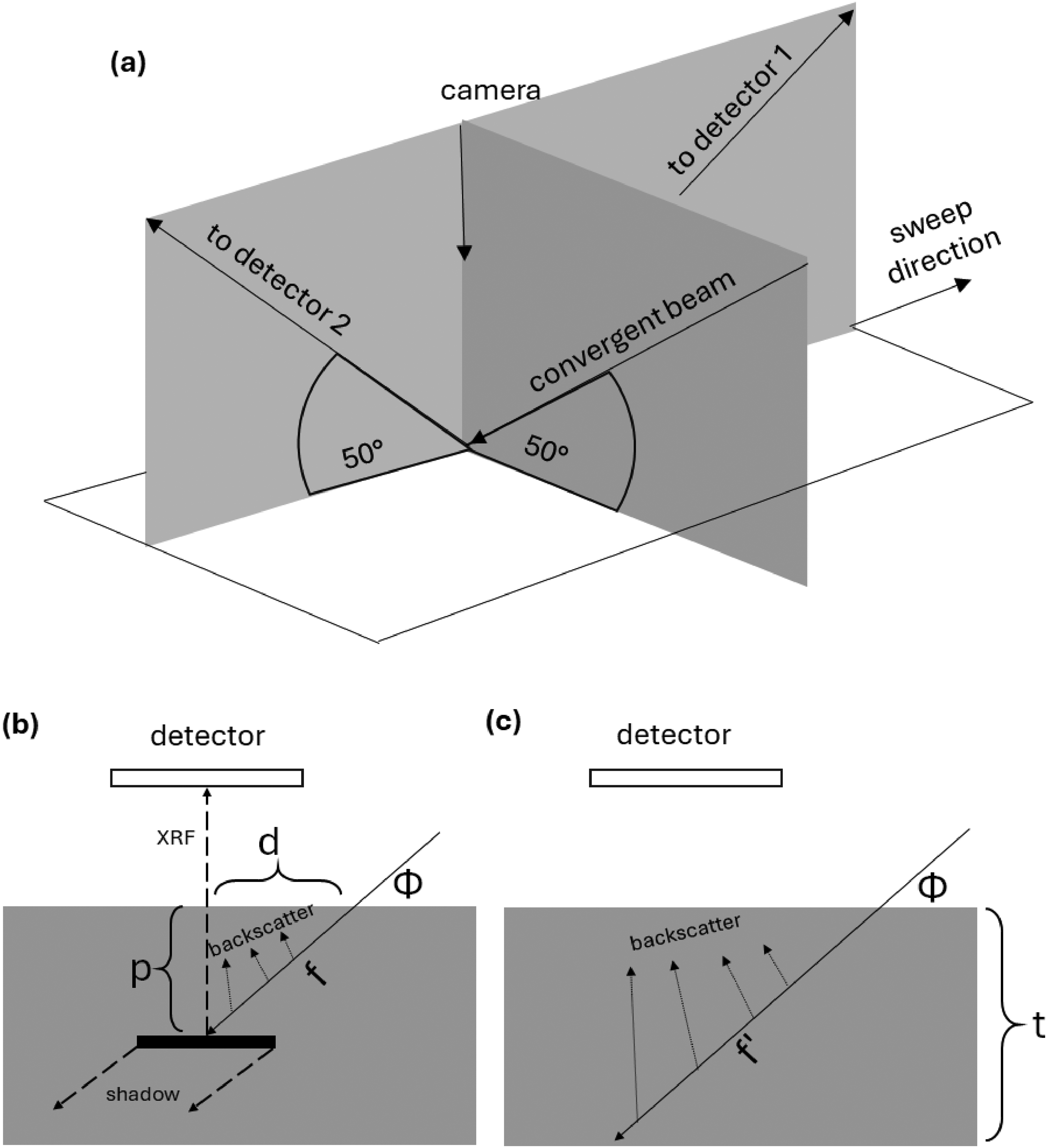
(a) Geometrical setup for commercial μXRF used, (b) X-ray fluorescence of internal object at a depth p and X-ray backscattering from a short path f through the sample matrix, (c) X-ray backscattering from a long path f ′ through the sample matrix. t is the thickness of sample and Φ is 50°. Note that detector is not in the same plane as the incident X-ray beam.

Sample preparation

Volumetric phantoms for qualitative analysis

Two different samples were prepared for qualitative analysis. The first sample was nearly spherical, made from wheat flour dough, with an embedded Cu-alloy cylinder. Wheat flour dough was chosen for the volumetric phantoms due to its ease of molding and its elemental composition, which is typical of plant tissues. The dough is primarily composed of C, H, O, and N (Z ≤ 8), with significant concentrations of K and Ca (Z = 19 and Z = 20). These latter elements produce easily detectable X-ray fluorescence in plant materials in the range of 3.3 to 4 keV. To the best of our knowledge, this is a novel approach for creating volumetric phantoms in μXRF studies. To reduce the Compton effect resulting from the Polymethyl methacrylate (PMMA) composition of the Tornado M4’s sample carriage, the sphere was placed on a 20 mm long metal support composed of Fe, Cu, and Zn. The second sample was also made from wheat flour dough but had an internal air gap. This sample was directly placed on the PMMA sample holder without the use of any metal support.

Flat phantom for quantitative analysis

A third sample, intended for quantitative analysis, was constructed through the superposition of three flat layers of PMMA, each with a thickness of 2.0 mm. These layers were secured at the edges with steel clips. This sample is shown schematically in Figure 2. At the interface between the first and second layers (a depth of 2.0 mm), a circular silver sheet and a tungsten sheet were inserted. Each of these sheets was 25 μm thick with a diameter of 6.3 mm. At the surface, an aluminium rectangular sheet approximately 30 μm thick was secured with methacrylate adhesive. Additionally, each PMMA layer was perforated with two 3 mm diameter holes for further analysis.

OPEN IN VIEWER

Figure 2.

PMMA-matrix flat sample schematical configuration including 4 metallic objects and 6 holes.

Workflow overview

The overall process flow for the acquisition, processing, analysis, and visualisation is described in Figure 3. This flowchart outlines the structured approach of the main processing steps and the associated activities carried out in each processing step. These steps are detailed in the following subsections.

OPEN IN VIEWER

Figure 3.

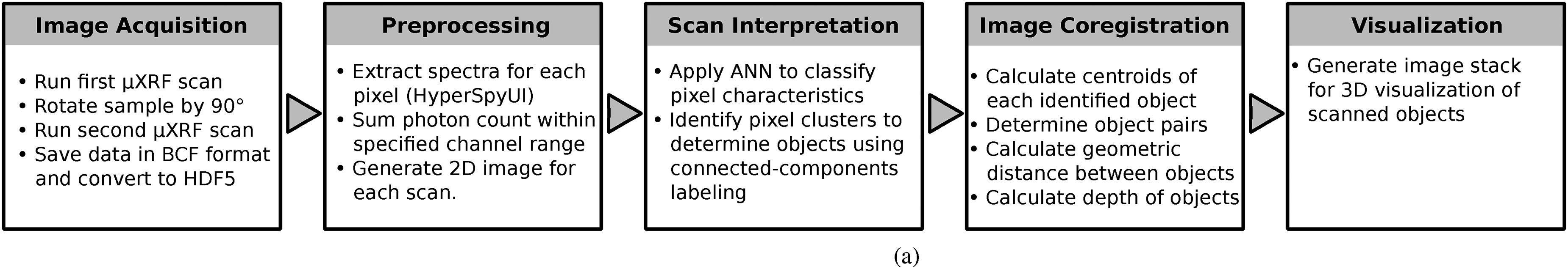
Flowchart showing the main processing steps and the associated activities.

Image acquisition

Two sequential orthogonal scans were performed on each sample. Initially, we conducted a scan, followed by a 90° clockwise rotation of the object in the XY plane, and then performed a subsequent second scan. The geometry of the μXRF device is depicted in Figure1(a). During the cartographic scan, the theoretical size of the focal spot was 20 μm. The spacing between spots, determined by the user, required balancing spatial resolution and scan duration. For this application, a spacing of 100 μm was selected, resulting in maps of approximately 400 × 400 pixels. Each pixel was scanned for 20 ms, resulting in a total scanning time of approximately 1.5 hours per scan.

The resulting data were saved in the Bruker hypermapping file format (BCF). The BrukerDataLibTest application (Bruker Corp.) was used to split these files into two new BCF files, one for each detector. These four BCF files were then imported into HyperSpyUI ²⁶ for further processing and converted into Hierarchical Data Format (HDF5). Only the data from detector 1, located upstream of the scanning movement, was used in this procedure.

Preprocessing

A preprocessing step was necessary to ensure the data were in a suitable format for the subsequent workflow. Custom scripts developed in RStudio ²⁷ were used to read the HDF5 files. These scripts, based on the rhdf5 library provided by Bioconductor.org, ²⁸ extracted the spectrum for each pixel and summed the photon count to generate a 2D image, represented as a 2D array. These resulting arrays (the second array being rotated by 90°) were saved in Comma Separated Values (CSV) format for subsequent viewing and analysis.

Scan interpretation

The images generated from each scan were analyzed to determine the elements in the sample. Each pixel was individually analyzed, and a classification was applied. The pixel classification process was carried out using an artificial neural network (ANN). In the examples studied in this paper, a limited number of elements were considered, and an ANN was trained to specifically identify this subset of materials. The training process involved manually labeling a series of 2D images of photon counts with the corresponding elements observed in the images. The labeled dataset was split into training (80%) and validation (20%) sets. Through a regularization process, a hidden layer size of 20 neurons was determined as the optimal number of neurons for the ANN, using the t a n h ( ⋅ ) activation function. The model was trained with a maximum of 1000 iterations or until convergence led to little improvement in the model fitting procedure. The model’s performance was evaluated using accuracy and F1-score metrics on the validation set. A number of different network architectures were considered, but from some preliminary analysis, it was determined that the chosen setup was the most suitable configuration.

Once all pixels in the 2D image arrays were classified, clusters of similar pixels were identified using connected-component labeling, ²⁹ a method that scans an image and groups its pixels into components based on a pixel connectivity measure. In this case, pixels classified as the same material or element were grouped or labelled as distinct objects. ³⁰

All computational tasks related to image analysis, including the neural network calculations, were performed using software written in Python and common libraries such as NumPy, ³¹ SciPy, ³² scikit-learn, ³³ and OpenCV.^34,35

Image coregistration

Image coregistration is the process of geometrically aligning two or more images to ensure that corresponding pixels representing the same objects are accurately matched, allowing for their integration or fusion.

First, the centroids of each identified object, i.e., the centers of the fully connected pixel objects, were computed. This computation was relative to a fixed origin in the image, providing a uniform reference point for subsequent analyses.

Next, identical objects across different images were matched. This step involved determining object pairs based on their centroids. The matching algorithm utilized a nearest-neighbor approach, where each object in one image was paired with the nearest object in the other image based on the Euclidean distance between their centroids. In cases where objects were missing in one of the images, the algorithm treated them as outliers and excluded them from further analysis. Following this, the geometric distances, dx and dy, between these matched objects were computed.

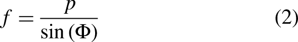
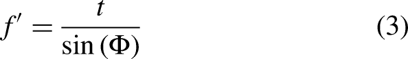
Finally, the depth (p) of the objects was calculated. Using the computed distances, dx and dy, the depth, as shown in (Figure 1(b)), was determined according to:

p = d ⋅ tan ( Φ )

(1)

where Φ refers to the tilt angle of the X-ray convergent beam, set at 50° in our experiments, and d the Euclidean distance, is calculated as either the distance of dx or dy. This relationship acknowledges that the recorded and actual positions of an internal flat object will differ more significantly as the object’s depth within the sample increases. The distances dx and dy were orthogonal between both images, thereby enabling the calculation of the object’s real position and two different depth predictions. This process effectively accounted for the stereoscopic effect of either XRF or Compton scattering, depending on the energy range analyzed.

Visualization

The final step in the process was to create an image stack. This was performed after determining the depths of all the objects in the images. The image stack serves as a powerful visualization tool, providing a comprehensive three-dimensional perspective of the object arrangement within the samples by using the ImageJ software image stack functionality. ³⁶

Results

Qualitative results

Prediction of the resulting contrasts

In the predictive analysis performed for this study, the sample’s matrix was composed of elements with atomic numbers (Z) less than or equal to 20 (i.e. C, H, O, K, Ca). In this setup, we consider it infeasible to use a matrix with elements heavier than Z = 20, unless the embedded objects correspond to heavy metals. The internal object used in this setup, however, was a homogeneous structure with a Z value greater than 20. The practical detection limit for light elements in SDD is above 1.4 keV in air, corresponding to Z ≥ 13 (Kα aluminum = 1.49 keV). When the inclined Φ degrees polyenergetic convergent-beam impinges on the flat object at depth p within a light matrix of thickness t, the attenuated beam on a path:

f = p sin ( Φ )

(2)

generates fluorescence on this surface (Figure 1(b)). A proportion of this fluorescence escapes towards the non-collimated detector after being attenuated by the matrix. Also during the path f, photons are scattered through Compton effect and Rayleigh scattering from the light matrix, a portion of which will reach the detector. We consider that all photons that reach the detector come from either X-ray fluorescence or Compton scattering. The Compton scattering angle θ varies, with a wider range if f is larger, the detector area is larger, or if it is closer. Scattering processes within the internal object occur, though less intensely due to the higher atomic number compared to the surrounding matrix. Furthermore, secondary X-ray interactions, such as X-ray fluorescence from elements excited by the primary X-rays, will occur within the sample, and their photons could potentially reach the detector. However, these effects are deemed negligible for the simplicity of our model.

It is important to note that while the current study focuses on light matrix samples, the proposed method could potentially be applied to materials with higher attenuations. In such cases, the method may be effective in detecting inclusions that emit higher energy XRF, such as heavy metals. The contrast in Compton backscattering intensity between the matrix and the inclusions, along with the X-ray fluorescence emission from the inclusions that manage to escape the matrix, would still form the basis for detection and analysis. However, further research is needed to validate the applicability of the method to high-attenuation materials and to establish its limitations in such contexts.

If the convergent beam in the internal path is not interrupted by any object with Z ≥ 13 , no detectable fluorescence will be produced. The Compton effect will be relatively more intense since it traverses a path:

f ′ = t sin ( Φ )

(3)

through the light matrix that is greater than f (Figure 3(b) and (c)), given t as the thickness of sample and Φ as the inclination of the polyenergetic convergent beam. Consequently, an object with Z ≥ 13 will contrast with the surrounding matrix in the energy ranges where Compton scattering is predominant. The contrast will decrease as the depth p of the object increases, eventually becoming indistinguishable if the object is located deeper than a certain threshold.

Volumetric phantoms

Figure 4 presents the accumulated spectrum of detector 1 for sample 1. The Compton effect of the source Bremsstrahlung is predominant in the range of 1015 keV for the supply voltage of 50 kV. Meanwhile, the Compton backscattering of the characteristic lines of Rh shifts to 18.9 and 21.2 keV for the given setup. An object with Z ≥ 13 will be brighter than the surrounding matrix in the analysed energy range from 1.4 to 25 keV. As before, this contrast will decrease as p increases, becoming indistinguishable, if the object is deep enough. These contrasting tendencies in different energy ranges enable the detection of the presence and shape of an object less dense than the matrix and the determination of its elemental composition.

OPEN IN VIEWER

Figure 4.

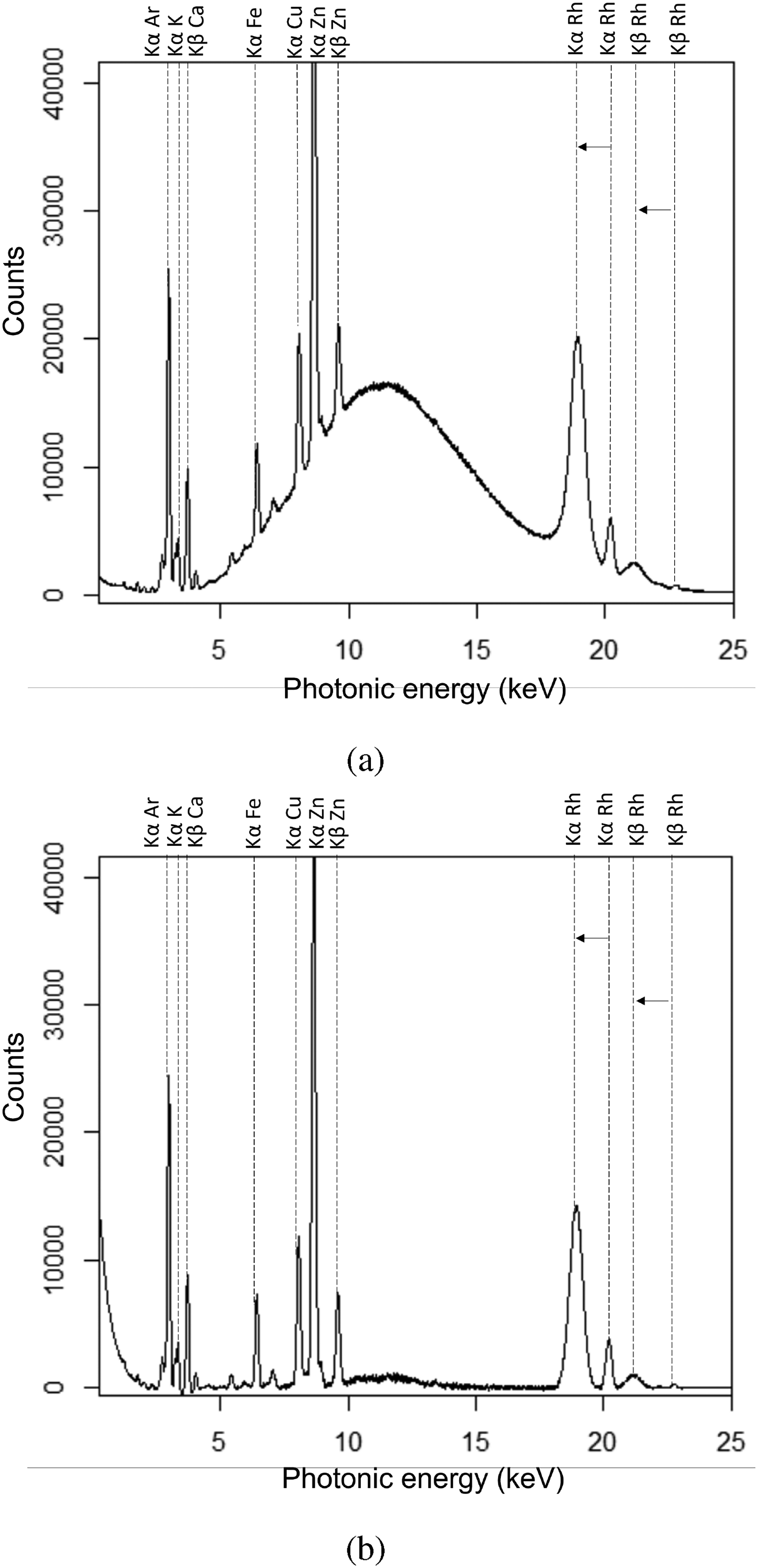
(a) Accumulated spectrum for detector 1 for sample 1. (b) Same spectrum corrected for baseline suppression using the fillPeaks method from the baseline library in RStudio.

While this study focuses on a light matrix sample, the method could potentially be applied to materials with higher attenuations. In such cases, the method may be effective in detecting inclusions that emit higher energy XRF, such as heavy metals. The contrast in Compton backscattering intensity between the matrix and the inclusions, along with the X-ray fluorescence emission from the inclusions that manage to escape the matrix, would still form the basis for detection and analysis.

The X-ray fluorescence of the light elements that composes the matrix such as K and Ca can be easily distinguished. Additionally, intense fluorescence of Fe, Cu and Zn originates both in the embedded metal and in the support. Between 10 and 12 keV is the maximum of the backscattering of the Bremsstrahlung (Figure 4(a)). At 18.9 and 21.2 keV, the Compton peak of the Kα and Kβ lines of Rh emerges, and between both, at 20.2 keV the Raleigh Kα peak of Rh (Figure 4(b)). Figure 5 presents images for samples 1 and 2, constructed from the sum of the channels in different energy ranges. For sample 1, Figure 5(a) shows the Kα emission of calcium (Ca), presenting a surface image due to its low penetration capacity. Figure 5(b), corresponding to Cu Kα, detects the presence of the embedded object and the fluorescence of the support. Finally, in the Compton backscattering image (Figure 5(c)), the materials with high Z (embedding and support) generate low intensity due to Compton scattering of the Rh Kα line, creating a contrast with the low-Z matrix. For sample 2, Figure 5(d) corresponding to Ca Kα presents the same surface view. Meanwhile, in the Compton backscattering image (Figure 5(e)), an internal void is clearly visible. This void does not generate X-ray fluorescence in any spectral range, enabling its detection. In Figure 5(e), unlike Figure 5(c), there is low contrast with the background due to the proximity of the sample holder surface, which is PMMA. The observed shadows result from the obstruction by the sample itself.

OPEN IN VIEWER

Figure 5.

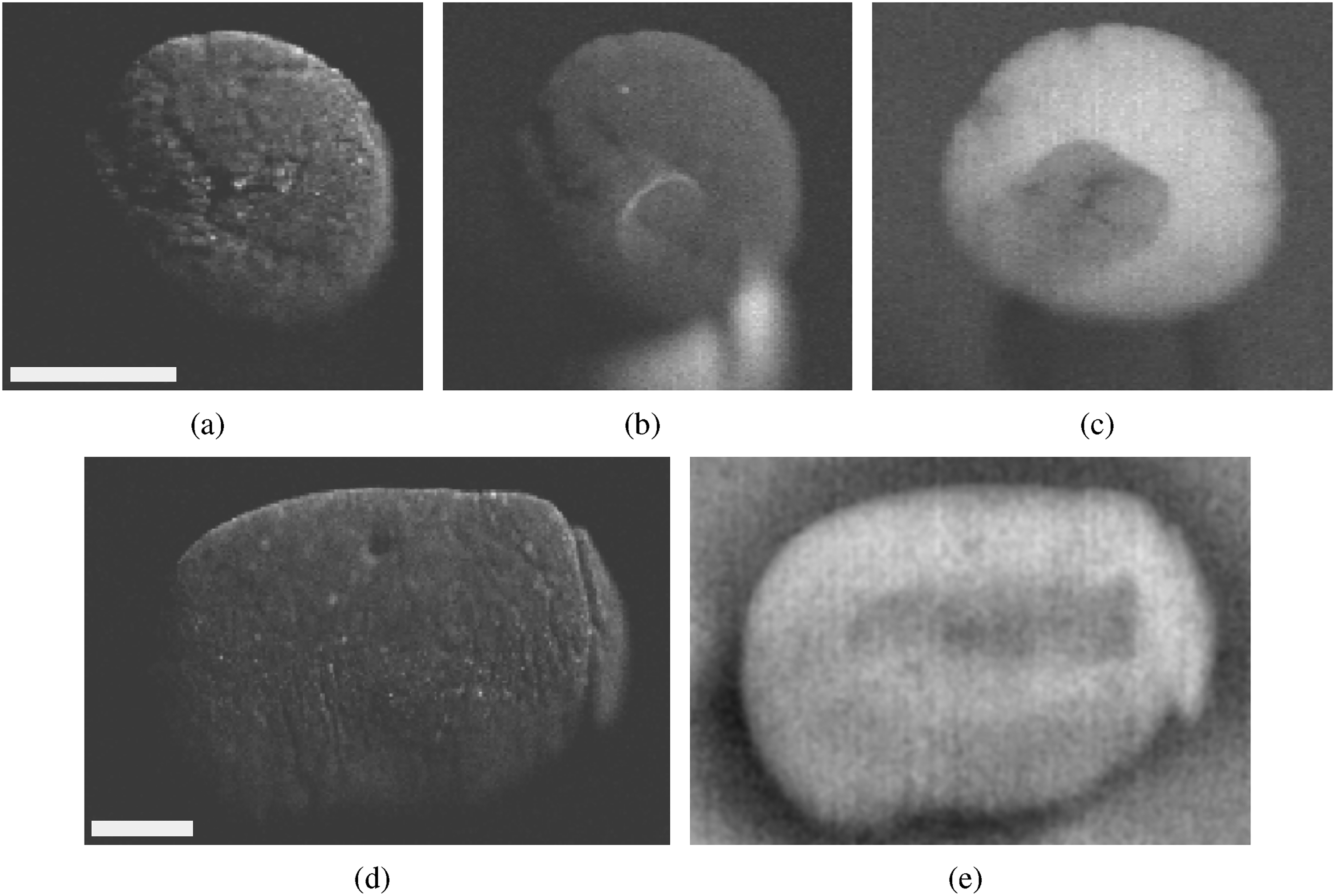
Wheat flour dough sphere with embedded copper cylinder (a) around 3.7 keV (b) around 8.0 keV and (c) around 19.0 keV (d) elongated sample of wheat flour dough with central void around 3.7 keV (e) around 19.0 keV (post-processing with CLAHE and smoothing). Note: White bars represent approximate 3 mm.

Flat phantom

Figure 6 presents the accumulated spectrum of detector 1 for sample 3. The Kα emission of Al, Cu and W are clearly distinguished. The emission Ag L (2.98 and 3.15 keV) is not detectable since it is superimposed with Ar K from the layer of air (2.96 and 3.19 keV). This superposition occurs because the energies of the Ag L and Ar K emissions are very close, and the resolution of the detector is not sufficient to separate them. The peak of Bremsstrahlung backscattering is in the range of 1012 keV. At 18.9 and 21.2 keV appears Compton peaks Rh Kα and Rh Kβ. Between both, at 20.2 keV the Raleigh Rh Kα appears, and Ag Kα at 22.2 keV.

OPEN IN VIEWER

Figure 6.

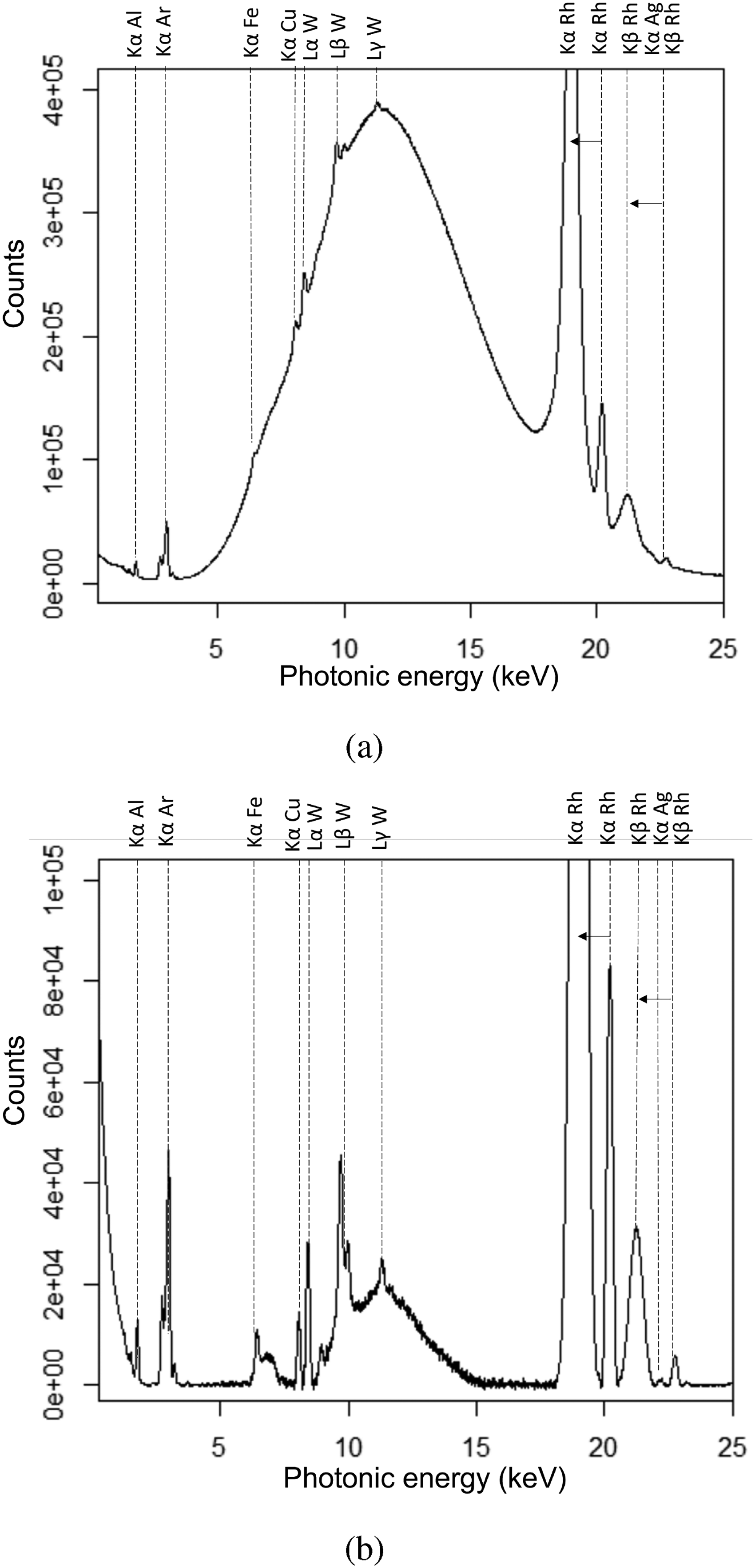
(a) Accumulated spectrum for detector 1. (b) Same spectrum corrected for baseline suppression using the fillPeaks method from the baseline library in RStudio.

Figure 7 presents images derived from summing channels over a range of energy spectra. Al K (1.5 keV) is highlighted in Figure 7(a) and (b). Copper (8.05 and 8.9 keV) and tungsten (8.4 keV) X-ray fluorescence is emphasized in Figure 7(c) and (d). Meanwhile, the fluorescence of silver (22.16 keV) is prominently displayed in Figure 7(i) and (j).

OPEN IN VIEWER

Figure 7.

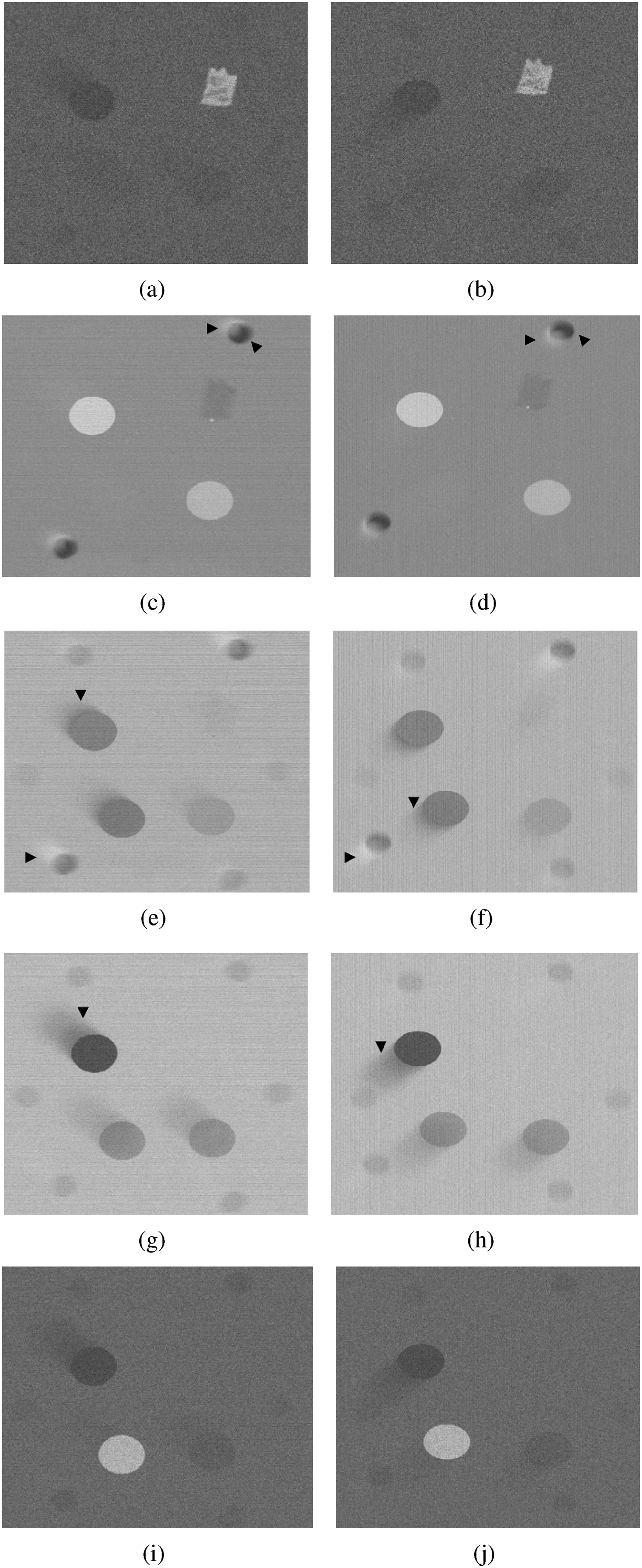
(a) Rotated horizontal scan from 1 to 2 keV, (b) Vertical scan from 1 to 2 keV, (c) Rotated horizontal scan from 7 to 9 keV, (d) Vertical scan from 7 to 9 keV, (e) Rotated horizontal scan from 11 to 14 keV, (f) Vertical scan from 11 to 14 keV, (g) Rotated horizontal scan from 18.2 to 19.6 keV, (h) Vertical scan from 18.2 to 19.6 keV, (i) Rotated horizontal scan from 21.5 to 22.5 keV, (j) Vertical scan from 21.5 to 22.5 keV. Note 1 : three circular high-Z objects have 6.3 mm of diameter. Note 2: Horizontal arrows: glares due to voids, tilted arrows: inward shadows due to voids, vertical arrows: shadows due to high-Z objects.

However, for energy ranges between 11 keV and 20 keV, Compton scattering becomes more prominent. This scattering effect is stronger for the PMMA matrix than for metals, resulting in metallic objects appearing in darker shades. This effect is noticeable in Figure 7(e)–(j) for copper and tungsten, and Figure 7(e)–(h) for silver.

In certain images, notably Figure 7(e) through (h), a dark shadow appears to be cast from each metallic object. In the images without rotation Figure 7(f), (h) and (j), these shadows are cast downwards and to the left. This directional shadowing aligns with the path of the tilted X-ray convergent beam, which approaches ‘from below’, and the location of detector 1, positioned to the right.

As expected, the holes in the PMMA matrix appear darker than the surrounding material, particularly noticeable in Figure 7(e)–(j). Yet, in Figure 7(c)–(d), the holes seem to create an optical illusion of depth.

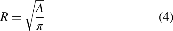
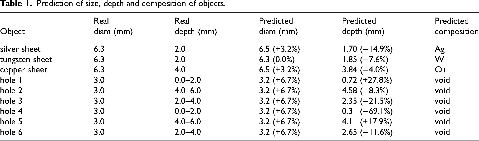
Figure 8 and Table 1 present the results of the prediction of the shape, size, depth and composition of the metallic objects embedded in the flat sample. The predicted radius, R, was calculated as

R = A π

(4)

where A refers to the total surface area of the identified object. The depth prediction corresponds to the average of the two orthogonal predictions. Percentage differences, Δ were calculated as:

Δ = ( d ~ − d ) d × 100

(5)

where d ~ is the estimated diameter and d the actual diameter of the object. Positive Δ values indicate overestimation, and negative Δ values indicate underestimation.

OPEN IN VIEWER

Figure 8.

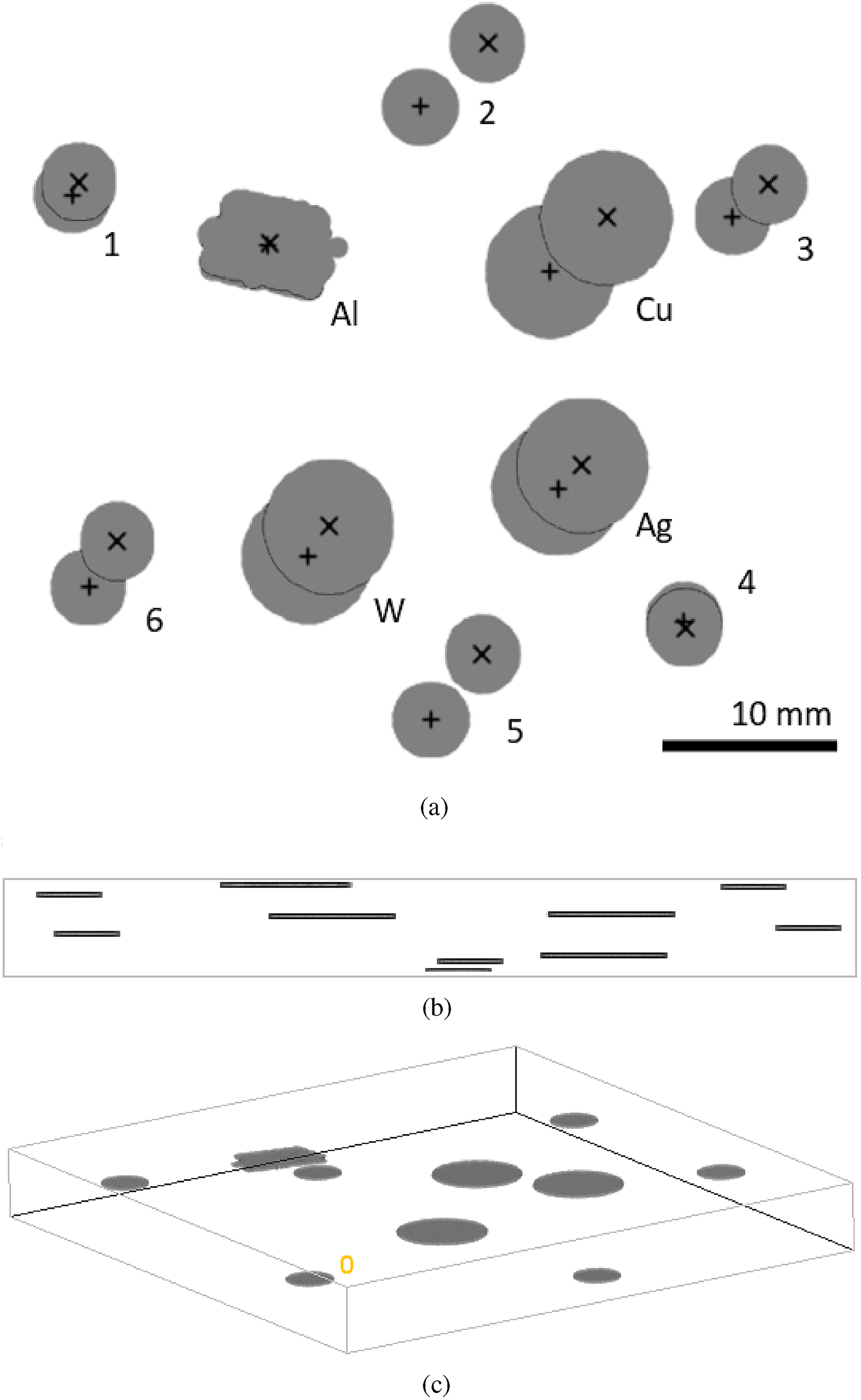
3D visualisation of recovered topographical arrangement of materials in Sample 3. In S1 of Supplementary material is provided a animation of these position’s distortions. In S2 of Supplementary material is provided a time-lapse animation for identification of objects by way of X-ray fluorescence and Compton backscattering. (a) Apparent positions for 4 metallic objects and for 6 holes for each perpendicular scan. Symbols (x) and (+) represent centroids for each scan. (b) Side view showing depth’s predictions. (c) 3D view of predicted positions and depths for all 10 objects.

OPEN IN VIEWER

Table 1.

Prediction of size, depth and composition of objects.

	Real	Real	Predicted	Predicted	Predicted
Object	diam (mm)	depth (mm)	diam (mm)	depth (mm)	composition
silver sheet	6.3	2.0	6.5 (+3.2%)	1.70 (−14.9%)	Ag
tungsten sheet	6.3	2.0	6.3 (0.0%)	1.85 (−7.6%)	W
copper sheet	6.3	4.0	6.5 (+3.2%)	3.84 (−4.0%)	Cu
hole 1	3.0	0.0–2.0	3.2 (+6.7%)	0.72 (+27.8%)	void
hole 2	3.0	4.0–6.0	3.2 (+6.7%)	4.58 (−8.3%)	void
hole 3	3.0	2.0–4.0	3.2 (+6.7%)	2.35 (−21.5%)	void
hole 4	3.0	0.0–2.0	3.2 (+6.7%)	0.31 (−69.1%)	void
hole 5	3.0	4.0–6.0	3.2 (+6.7%)	4.11 (+17.9%)	void
hole 6	3.0	2.0–4.0	3.2 (+6.7%)	2.65 (−11.6%)	void

Discussion

According to the manufacturer, given the present beam divergence of the polycapillary X-ray lens, defocused spot sizes ranging between 100 and 200 μm can be achieved by positioning the sample approximately 2-3 mm depth. ³⁷ From a quantitative perspective, this implies a divergence angle in the estimated range of 0.8°–2.6°. Theoretically, an increased spot size could contribute to a reduction in the sharpness or acutance of the detected objects that are located deeper within the sample. However, the results presented in Figure 7 do not align with this theoretical assumption. The acutance of objects positioned at depths of 2 mm (Ag and W) and 4 mm (Cu) is observed to be relatively similar. This apparent contradiction suggests that the spot size increase may not significantly affect the acutance of deeper objects within the established depth range. Future work could focus on examining the impact of spot size variation on the acutance of deeper objects under varying experimental conditions. Exploring a range of depths beyond the 2–4 mm used in this study will help establish a more comprehensive understanding of the divergence angle’s effect on image quality and the practical limitations of the technique.

When a section of the X-ray beam’s path is obstructed by an internal object, the attenuation of matrix backscattering increases, resulting in darker tones and casting a shadow artifact (as shown clearly in Figure 7(g) and (h)). In Figure 7(g), these shadows appear inclined approximately 45° to the left and up because the X-ray beam is incident from below, while the detector is on the right. In Figure 7(h) these shadows appear inclined to the left and down, because this image was rotated 90° counter clockwise for consistent representation.

As noted, the holes in the PMMA matrix appear darker that the neighbouring material. This effect is likely due to a combination of higher (dark area) and lower (light area) attenuation of Compton photons near the hole, as was discussed in earlier in the section predicting the resulting contrasts. This contrast of light and dark shadows, coupled with an absence of fluorescence response, identifies these areas as voids in the material.

It would be interesting to analyze the performance of the methodology used in this study on a diverse range of materials and object configurations, such as geological samples with multiple mineral inclusions or biological specimens with complex internal structures. Investigating the efficiency of detecting overlapping objects at various depths could provide insights into the strengths and limitations of the current approach and identify potential areas for improvement.

In the case of voids and holes, they will be barely distinguishable from the surrounding matrix if they are very thin. If they are thick enough, they will contrast with the matrix, appearing darker due to either a lack of fluorescence or the almost non-existent Compton effect from the air. Thus, voids could be differentiated from high-Z regions based on several characteristics: (i) voids will not fluorescence, (ii) voids will not cast shadows away from them, (iii) when the X-ray beam enters a surface void and strikes one of its walls, it will produce an inward shadow (Figure 7(c)–(f)), and (iv) when the X-ray convergent-beam impinges near the front edge of a surface void, it will create a glare due to the reduction of attenuation of Compton backscattering (Figure 7(c)–(f)).

During routine μXRF mapping, the tilted X-ray beam geometry coupled to non-collimated detector can create several artifacts. The main one is the mismatch between the images of the camera and μXRF. This shift can be reduced by focusing correctly or through post-processing. Currently the object detection methodology works around a fixed point in both images, significantly reducing the complexity of alignment between the two images. An alternative step should focus on image alignment based on the detected objects, rather than a fixed point.

Additionally, deep regions capable of emitting X-ray fluorescence will be mapped in position other than where they actually are. In attempts to make quantitative estimates of concentration from μXRF mapping there is potential for contrast artifacts that can lead to a misinterpretation of accumulations of elements. Some identifiable cases include: (a) Regions with high capacity to attenuate the X-ray will produce screening or shadow areas around them, which could be interpreted as areas with a low concentration of other elements. This will be more pronounced for lighter elements due to their lower X-ray fluorescence energy. (b) Regions of low attenuation, voids, or gaps can generate glows in their surroundings which can be misinterpreted as areas of high concentration.

Currently, to mitigate these artifacts, μXRF manufacturers propose cumulative counting of two detectors located in opposite positions, to attempt to capture what “one detector does not see, the other sees”. Although this two point of view approach does not completely solve these artifacts. Conversely, our orthogonal-tilted scanning approach can facilitate the interpretation of these anomalies.

Conclusion

In this study, we demonstrated the feasibility of using an off-the-shelf μXRF device for stereoscopic X-ray imaging of XRF and Compton backscattering without any hardware modifications. This proof-of-concept highlights the potential for expanding the capabilities of existing μXRF devices and opens up new avenues for non-destructive 3D imaging of complex samples. The results provide a foundation for developing improved and more advanced techniques for μXRF mapping that maintain high acutance at greater depths, enable the detection of a wider range of elements, and provide more comprehensive data on the 3D distribution of chemical components within a sample. These advancements have the potential to enhance the field of X-ray fluorescence imaging, enabling new research questions to be addressed in materials science, archaeology, biology, and other disciplines where non-destructive 3D chemical mapping is crucial.

Supplemental Material

Supplemental Material