How Representative Is the ACTIVE Sample? A Statistical Comparison of the ACTIVE Sample and the HRS Sample

Abstract

Objective: This research is designed to examine demographic differences between the ACTIVE sample and the larger, nationally representative Health and Retirement Study (HRS) sample. Method: After describing some relevant demographics (age, education, sex, and race/ethnicity), we use three statistical methods to determine sample differences—logistic regression modeling (LRM), decision tree analysis (DTA), and post-stratification and raking methods. When some differences are found, we create sample weights that other researchers can use to adjust these differences. Results: The ACTIVE sample is younger, more likely to be female, Black, and more highly educated than the HRS sample. Sample weights were created. Discussion: By using the resulting sample weights, all results of ACTIVE analyses can be said to be nationally representative based on HRS demographics.

Keywords

demographics statistical methods sample weights nationally representative sample ACTIVE

Introduction

The ACTIVE study was designed to test the transfer effects of cognitive training on everyday abilities in older adults (see Ball et al., 2002; Jobe et al., 2001; McArdle & Prindle, 2008; Rebok, Carlson, & Langbaum, 2007). Various assertions were made at the outset of the ACTIVE program of research: (a) The sample would be large enough to obtain precise estimates of training—with n > 2,800, this aim seems achievable; (b) the individuals were randomly assigned to three different training interventions and a no-contact control group—this randomized trial design allows direct comparison of groups of trained and not-trained individuals with unambiguous results, and this also seems to have been achieved; (c) the effects of cognitive training will transfer to measures of everyday functioning through their effects on cognitive abilities—this assertion has been tested at all occasions with evidence of transfer at 5 and 10 years after training was conducted (see McArdle & Prindle, 2008; Rebok et al., 2007; Willis et al., 2006); (d) the study enrolled a volunteer sample of older adults, with targeted efforts to include African Americans as they had been underrepresented in prior cognitive aging research—how representative the sample is of the older U.S. population has not been examined fully, a limitation for inferences of study findings; (e) the cognitive training programs are effective for a national population—this assumption also has been underlying all inferences, but it has not yet been fully examined.

The ACTIVE sample and resulting data set was created by asking a number of persons (more than 5,000) to participate and enrolling 2,802 participants. The subsequent randomization to four groups brings each group to about 700 in number. Whereas we assume that the initial sampling reflects some form of participant sampling bias itself, we do not pursue this matter further. We also do not pursue the analysis of the randomized treatments as this has been reported elsewhere (Ball et al., 2002; Willis et al., 2006). What is pursued here is an assessment of the national representation of the participants in ACTIVE.

The idea that results from the selected sample of people can generalize to the entire population of older adults is of obvious importance for a study of this magnitude. Many recent claims have been made about the growth and decline of specific cognitive functions (e.g., Horn, 1967; Kaufman, Kaufman, Liu, & Johnson, 2009; McArdle, Ferrer-Caja, Hamagami, & Woodcock, 2002; Schaie & Willis, 1993; Zimprich & Martin, 2002), but the national samples used in these studies were all assumed to be representative of some important population. As far as we can tell, these key assumptions were not fully examined.

To examine the presumption that the ACTIVE sample is nationally representative, it is compared with the sample of the Health and Retirement Study (HRS; Juster & Suzman, 1995; McArdle, Fisher, & Kadlec, 2007), considering the HRS sample as a proxy for a nationally representative distribution of people. To carry out these analyses, we use publicly available data (from ICPSR/NACDA) for ACTIVE and HRS studies (see ICPSR/NACDA and HRS websites) to collate comparable sample demographic characteristics (age, education, sex, race/ethnicity) for each study sample. To see whether there is any deviation between the two studies, we use three approaches: (a) logistic regression modeling (LRM to examine groups differences; (b) a more exploratory data-mining approach termed decision tree analysis (DTA), following (McArdle, 2011, 2012); and (c) the idea of weighing the sample to account for any deviations of the ACTIVE study from the HRS population characteristics with post-stratification and raking.

As a result, a new set of sampling weights (see Cole & Hernan, 2008; Kish, 1995) are obtained using the post-stratification, LRM, DTA, and raking approaches and applied to assess how the weights affect outcomes previously reported. Each process uses the same demographic variables that were used in the sample association analysis (age, education, sex, and race/ethnicity). To the degree that any subsequent analyses of ACTIVE data use these sampling weights, it can be said that the results of these analyses are as nationally representative as the HRS.

Method

Participants

The data were accessible from the University of Michigan ICPSR’s data repository and from the HRS database. From these files, the demographics for each person were available as outlined above. The data files were merged together, and years of age, years of education, sex, and race/ethnicity were equated between samples. For age, the sample of ACTIVE included persons aged 65 to 95 years (Jobe et al., 2001). Because the HRS age range was broader (about 50-95), the HRS sample was reduced to include only persons 65 to 95 years, to be directly in line with ACTIVE. The HRS restricted sample is N = 10,487.

Next, the demographic variables were recoded for simplicity and interpretation. The age variable was centered at 65 for all subsequent analyses. Years of education included the reported number of years of education through high school diploma (1-12), associate degree (14), bachelor’s degree (16), master’s degree (18), and the PhD/MD (20). The final Education variable was centered at 12. Sex was coded in the female direction, with males coded 0 and females coded 1. Race/ethnicity includes responses of White, Black, and Other, where White is the baseline (0), and Black (1) and Other (1) are simple contrasts allowing direct estimates of group differences.

Initial Data Description

The ACTIVE sample was defined in relation to the goals of the trial and not intended to be representative of the U.S. population. The sample was drawn from six metropolitan/surrounding areas (Birmingham, AL; Boston, MA; Indianapolis, IN; Baltimore, MD; State College, PA; Detroit, MI). Six locations were chosen to sample the various areas of the United States while maintaining close connection with participants to minimize the costs of conducting the training interventions. Each field site had a specific study population and recruitment strategy, including senior housing, service agencies, churches, healthcare facilities, and public records. African Americans were oversampled because of their low prevalence in prior research on cognitive training (Jobe et al., 2001). Participants had to be at least 65 years old, community dwelling, and generally healthy with no physical or mental disabilities that would prevent them from completing a training program and cognitive testing.

The HRS was designed to include a nationally representative sample of adults, generally 50 and older (see Juster & Suzman, 1995), as long as the sample weights are applied. In proposing a comparison of the HRS and ACTIVE samples, it is noted that the studies have similar aims in longitudinally following the trajectory of an aging population in the United States. The massive size of the HRS sample and the previous work to bring it in line with national population parameters mean that it serves as a good prototype for ACTIVE (Hauser & Willis, 2005). The HRS includes a great deal of demographic information, but for purposes of this analysis, we focus on the participant’s self-reported age, education, sex, and race/ethnicity. Age and education are reported in years (education in terms of years of formal schooling), and sex is listed as Male or Female. Race/ethnicity is indexed in several ways, and here we create subgroups of White, Black, and Other as shown in Table 1 for the HRS respondents over age 65.

Table 1.

Demographic Simple Statistics for ACTIVE and HRS.

A. ACTIVE sample demographic variables
				Ethnicity
	Age	Education	Sex	White	Black	Other
M	73.6	13.5	75.9%	72.4%	26.0%	1.64%
SD	5.91	2.77
n	2,802	2,802	2,802	2,028	728	46
B. HRS 2010 sample demographic variables^a
				Ethnicity
	Age	Education	Sex	Black	White	Other
M	76.1	12.3	58.3%	83.7%	13.9%	2.34%
SD	7.01	3.23
n	10,487	10,486	10,487	8,781	1,461	245

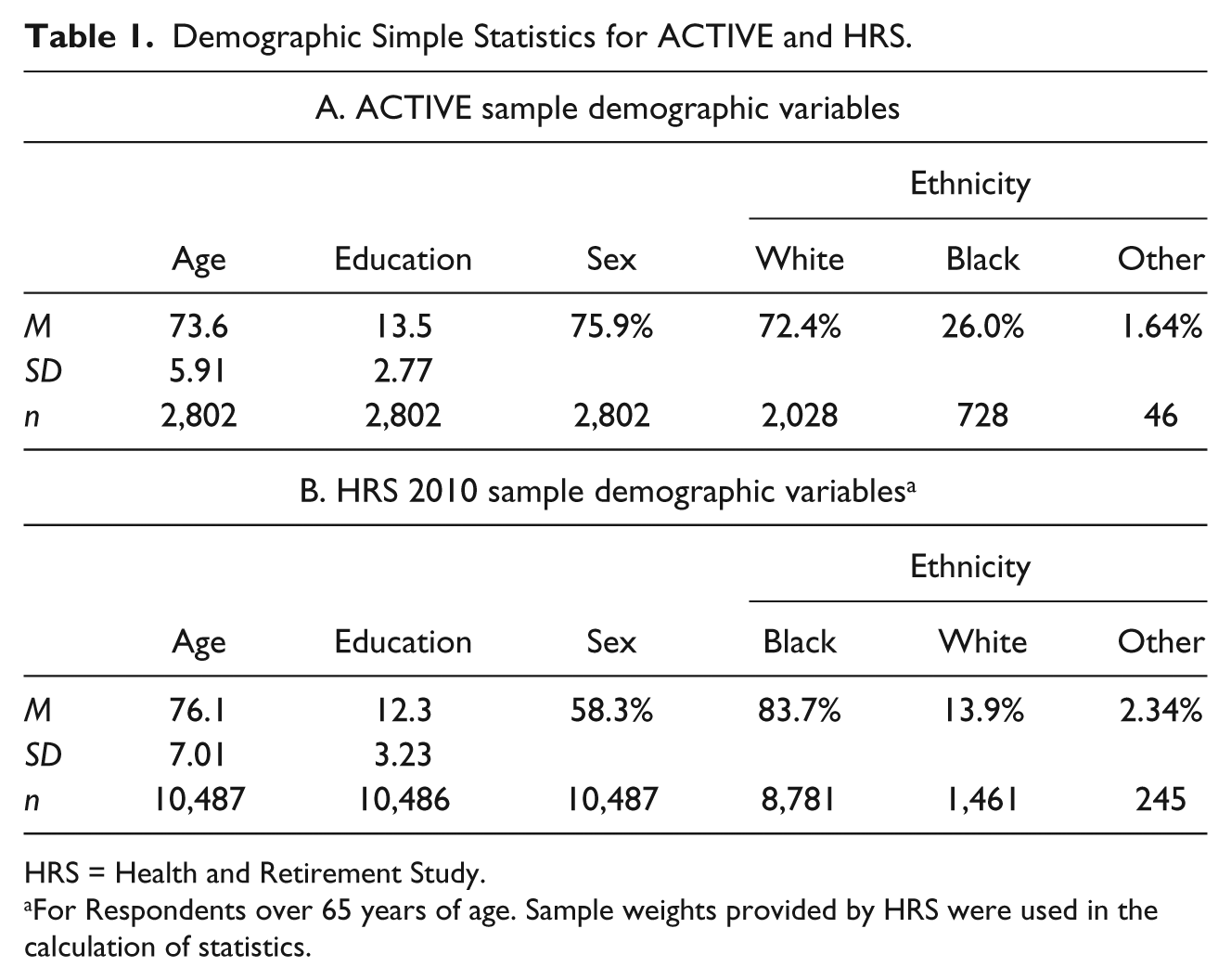
HRS = Health and Retirement Study.

For Respondents over 65 years of age. Sample weights provided by HRS were used in the calculation of statistics.

The Other category includes individuals who reported their race/ethnicity as Asian, Latino, or Native American. These subcategories were sampled in rather small percentages, leading to very small cell sizes when the data are further crossed with other variables. For a clear comparison of the sample demographics, the ACTIVE demographics are listed in the second part of Table 1. Here, the sample average age and education are listed next to the proportions of females (sex) and defined race/ethnic groups. Some of the last proportions show some differences, but these will be examined through the models of study association.

The ACTIVE study began enrollment in 1998, with 5-year assessments ending in 2004. The HRS began in 1992, providing that demographic similarities could be biased by effects of time (Juster & Suzman, 1995). To rectify the difference in initial sampling, the year 2000 sample and weights from the HRS were used as the prototype to compare with ACTIVE.

If the ACTIVE sample was found to have some biases for certain demographic proportions, we may wish to weigh the sample to bring these ACTIVE proportions in line with the HRS population. The first step in this process was to create brackets for age and education to have good coverage of each value across the spectrum of ages and years of education. These brackets are shown in Table 2. The brackets were created by grouping age in 5-year intervals from age 65 to 95 (the age range for ACTIVE), and they illustrate the potential nonlinearity of the predictors. The restrictions based on age for HRS from the previous analysis were carried over so that the age ranges were equal across groups. Additionally, bracketing age in this manner is a necessity for cell-based weight calculation methods (e.g., post-stratification and raking).

Table 2.

Demographic Brackets for ACTIVE Sample.

	Frequency	%	Cumulative frequency	Cumulative percentage
Age categories
65-69	819	29.23	819	29.23
70-74	864	30.84	1,683	60.06
75-79	609	21.73	2,292	81.8
80-84	372	13.28	2,664	95.07
85-89	119	4.25	2,783	99.32
90-94	19	0.68	2,802	100
Education categories
0-4 years	3	0.11	3	0.11
5-8 years	86	3.07	89	3.18
9-12 years	1,030	36.76	1,119	39.94
13 years	786	28.05	1,905	67.99
14 years	120	4.28	2,025	72.27
15 years	318	11.35	2,343	83.62
16+years	459	16.38	2,802	100

Note. The higher age brackets were collapsed (85-94) because of lower cell sizes. The same was true of the first two education categories.

Models of Analysis

The first part of the analysis deals with testing whether certain demographic variables predict study association (ACTIVE vs. HRS). This was done by implementing a logistic regression process where the outcome is study assignment (see Hosmer & Lemeshow, 1989; McArdle & Hamagami, 1994). Those that were included in the HRS are assigned 0 and those in ACTIVE are assigned 1. The sample demographics are used as predictors (age, education, sex, race/ethnicity). The analysis of study association was broken down into a few steps to progressively build a full model of predictors. Each predictor was put in individually to report a baseline in predicted variance (pseudo R²); a 5% level of significance is reported. After this, the complete set was input as a multiple logistic regression.

Next, a DTA using a Classification and Regression Tree (CART) approach was used to predict group association for the two studies (see McArdle, 2011, 2013). The historical view of DTA is presented in detail elsewhere (see Breiman, Friedman, Olshen, & Stone, 1984), and there are many available computer programs (see McArdle, 2011; Strobl, Malley, & Tutz, 2009). DTAs have a few common features: (a) They are admittedly “explorations” of available data; (b) in most DTAs, the outcomes are considered to be so critical that it does not seem to matter how we create the forecasts as long as they are “maximally accurate”; (c) some of the DTA data used have a totally unknown structure, and experimental manipulation is not a formal consideration; (d) DTAs are only one of many statistical tools that could have been used. Popularity of DTA comes from its easy to interpret dendrograms, or Tree structures, and the related Cartesian subplots. DTA programs are now widely available and very easy to use and interpret. The DTA used here was based on a CART classification method (R programs using “rpart” and “party”; Hothorn, Hornik, & Zeileis, 2006) with the binary outcomes of ACTIVE versus HRS and the demographics listed above as inputs. No utilities were used, so the sample sizes were not reweighed. Splitting on a given variable is done by selecting the variable that offers the maximal prediction of the outcome in a set of variable. These splitting potentials take into account data in categorical and continuous configurations. The analyses also include a comparison of the various weights and their effects on the demographics used (biases in means are examined).

In the post-stratification and raking methods, the general trend is to use cell-based proportions to reweigh underrepresented cells from the sample to match the population proportions (Holt & Smith, 1979). This procedure used sex- and age-ordered categories as the splits for cell association. Further division of cells by race and/or education created empty stratified cells in the sample. Alternatively, we can use a “raking” method (Deville, Sarndal, & Sautory, 1993) approach to make sample proportions more closely match the population proportions (in this case, those of the HRS). The raking process for creating the sample weights involves knowing the relative population proportions of the demographics that we are using in our analyses (age, education, sex, race/ethnicity). For this, we use the weighed HRS data (HRS proportions using the sample weights created for that data). The raking process iterates weights by smoothing out oversampled categories and increasing weights on undersampled portions. If at the end of the iterative process, the deviation of the weighing has not settled, new brackets should be made to account for low information cells. This technique can be thought of as a two-way post-stratification that rakes along columns and then along rows to progressively revise sample weights to match population proportions over separate cell divisions (Little, 1993).

Finally, to assess how these weights affect the intervention effects previously reported (Ball et al., 2002; Willis et al., 2006), results of unweighed repeated measures MANOVA are compared with the results of weighed repeated measures MANOVA, using weights obtained through the models described above. This provides the opportunity to determine how well the unweighed means match the weighed means. If the means change substantially, we have reason to believe that the proportion in the sample leads to biased results and is not generalizable to the general population and use of the weights would reduce this bias.

Results

LRM Analyses

Simple effects of individual predictors

The first set of results comes from logistic regressions with single predictors of study association (see Appendix Table 1). From this, we can see how well each variable predicts association without possible collinearity effects. A list of the results of single predictors for study association is displayed in Table 3. The logistic models the propensity of being enrolled in ACTIVE versus HRS as a function of age, education, sex, and race. Differences were detected, with lower ages and higher education in the ACTIVE sample. In addition, the ACTIVE sample was significantly more likely to be female than the HRS sample and to include significantly more Blacks than in the HRS sample.

Table 3.

Logistic Predictors of Study Association (HRS = 0, ACTIVE = 1).

	Single logistic indicators		Multiple indicators
Predictor	OR	95% CI	OR	95% CI
Age	0.945	[0.938, 0.951]	0.953	[0.947, 0.960]
Education	1.142	[1.125, 1.159]	1.173	[1.154, 1.193]
Sex	2.253	[2.049, 2.477]	2.354	[2.133, 2.597]
Race (B)	2.158	[1.950, 2.387]	2.201	[1.975, 2.452]
Race (O)	0.813	[0.591, 1.118]	0.91	[0.654, 1.268]

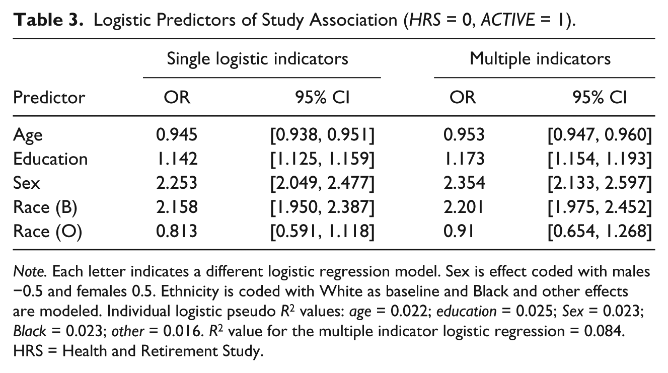
Note. Each letter indicates a different logistic regression model. Sex is effect coded with males −0.5 and females 0.5. Ethnicity is coded with White as baseline and Black and other effects are modeled. Individual logistic pseudo R² values: age = 0.022; education = 0.025; Sex = 0.023; Black = 0.023; other = 0.016. R² value for the multiple indicator logistic regression = 0.084. HRS = Health and Retirement Study.

In addition to these odds ratio estimates, we get a sense for the ability to discern study association with the pseudo R² values. Data in this table give us an idea of the ability of the predictor variables to correctly classify persons, rather than the amount of explained variance as in a traditional regression analysis. In this kind of comparison, these variables offer little evidence that we could correctly identify persons as being HRS or ACTIVE participants with any degree of certainty. But here, this result implies that there is very little bias in the sampling procedures between these two samples. Because these estimates are run as separate logistic regressions, we move to a multiple predictor model to see whether the results hold.

Main effects regression

In an effort to determine how well the demographic variables could capture person-study association, we implemented a multiple regression analysis, with age, education, sex and race/ethnicity entered as multiple predictors of study association. Results are presented in Table 3; overall pseudo R² = 0.084. The main effects of these variables in predicting whether a person was a member of the ACTIVE or HRS sample were similar to that of the single predictor models reported above. All main effects were significant, indicating many independent effects, and the only value that showed no bias between samples was the effect of the other race/ethnicity category. The overall effect of these variables to correctly classify persons is relatively low given the individual effects outlined previously. These results are in line with the previous analyses, but there is only a small gain of enhanced prediction with multiple predictors.

Interaction effects regression

The model was extended to include multiple predictors and all the two-way interactions of these same predictors. In the model, we look to see whether the main effects still hold, and how the interactions may change the interpretations stated in the previous two sections. Results are shown in Table 4.

Table 4.

Study Association Analysis With Two-Way Interaction Terms.

Predictor	β	SE	OR	95% CI
Age	0.026	0.027	1.026	[0.972, 1.082]
Education	0.260	0.062	1.296	[1.148, 1.463]
Sex	0.912	0.406	2.489	[1.124, 5.510]
Race (B)	0.482	0.053	2.623	[2.134, 3.225]
Race (O)	−0.574	0.186	0.317	[0.153, 0.658]
Age × Sex	−0.006	0.008	0.994	[0.978, 1.010]
Age × Education	0.001	0.001	1.001	[0.999, 1.004]
Age × Black	0.024	0.010	1.024	[1.005, 1.044]
Age × Other	−0.095	0.026	0.909	[0.864, 0.956]
Education × Sex	−0.082	0.019	0.922	[0.888, 0.956]
Education × Black	−0.011	0.020	0.989	[0.951, 1.029]
Education × Other	−0.091	0.058	0.913	[0.815, 1.022]
Sex × Black	−0.067	0.136	0.935	[0.717, 1.220]
Sex × Other	0.197	0.380	1.217	[0.579, 2.562]

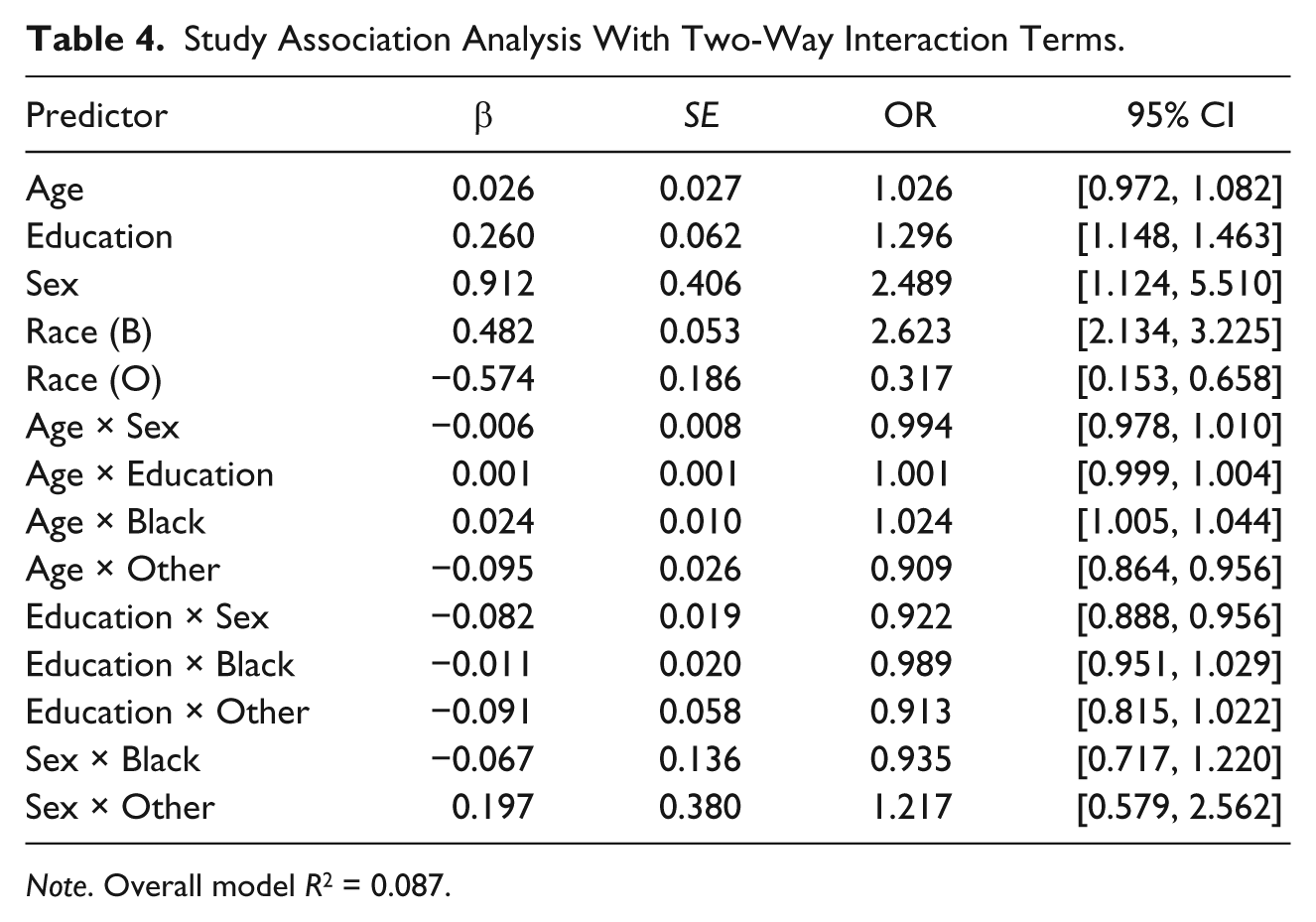
Note. Overall model R² = 0.087.

We note that the main effect of age is now not significant, but the effect of the interaction of age with each race/ethnic category is significant. The effects of education, sex, and Black race mimic the multiple regression results previously presented. The interaction of education and sex showed a disadvantage for males in the ACTIVE study versus the HRS sample.

The overall effect of adding two-way interactions provides little prediction value to the overall model (R² = 0.084 → 0.087) compared with the model when only main effects are included, so we will only use the main effects model. The pseudo R² provides a limited view of the differences between the two studies, with only about 8% of the prediction accounted for by the sample characteristics selected in the analysis. With a small effect given sample demographics for HRS and ACTIVE, we conclude that only minor differences exist between the samples.

DTAs

The same set of data was examined using data-mining techniques (see Appendix Table 2). In these models, we allow all possible nonlinear interactions between the demographic characteristics available. Study association was again listed as the predicted outcome, with the demographic variables of age, education, sex, and race/ethnicity used as predictors of the possible splitting nodes. The outcome of this analysis is a decision tree that splits persons into groups based on cut-points with continuous variables and on group with categorical variables.

The final tree is shown in Figure 1. This is based on 23 groups determined to have the best splits by “rpart” R program (see R Core Team, 2013; Strobl et al., 2009; Therneau, Atkinson, & Ripley, 2012). In this case, age provided the first split at age 65.04. Next, sex was used as a splitting variable, with females going to the left path. Then, education was used to split the data at 16 years of education, and then it was used again at 13 years of education for the lower branch. Therefore, the optimal tree that we found suggested age (13.4%), education (3.9%), sex (0.7%), and race/ethnicity (0.3%) to be important variables to organizing persons based on study association (with variable importance in the order listed). The overall accuracy of this DTA was 14.6%, a slight increase over the LRM of 8.4%. This shows the specific nonlinearity (especially within education) and the resulting higher order interactions between the variables that would not be apparent in simple two-way interactions portrayed in the above LRM.

Figure 1.

Snapshot of DTA-PARTY decision tree.

Post-Stratification and Raking Methods

The ACTIVE Time 1 data were used to create weights based on HRS weighed proportions. For the post-stratification method, the sex-by-age and sex-by-ethnicity proportions were used to create sample weights. The HRS proportions were divided by the ACTIVE proportions to return the relative weight to be given to each cell. If the proportion for older males was higher in ACTIVE than HRS, their weight would be less than 1 (indicating that this group is overrepresented).

A similar method of weighing was established for the raking process. For this, three interaction terms were created for sex by: age (12 cells), education (12 cells), and race/ethnicity (6 cells). When we establish that we essentially have three post-stratified proportions that we will “rake” over, it is more clearly identified as an extension of post-stratification. The raking procedure used these three interactions to create marginal sample weights for ACTIVE based on proportions from HRS with marginal weights. The stopping rule for raking included program termination when the calculated percentages differed from the marginal percentages by less than 0.001. This was established in 5 iterations when a maximum of 50 was requested.

Creating Sample Weights for ACTIVE

We create sampling weights from the LRM in the usual ways (see Cole & Hernan, 2008). Similarly, sampling weights can be easily created from the DTA output by assuming that the probability of inclusion in ACTIVE is the percentage of ACTIVE participants in the final nodes. In Table 5, we list a few sample statistics for the unweighted and weighted demographics in the ACTIVE sample. The LRM and DTA methods seem to yield values more in line with the original sample statistics unweighted.

Table 5.

Unweighted and Weighted ACTIVE Statistics.

A. Unweighted statistics
				Ethnicity
	Age	Education	Sex	White	Black	Other
M	73.6	13.5	75.9%	72.4%	26.0%	1.64%
SD	5.91	2.77
n	2,802	2,802	2,802	2,028	728	46
B. LRM weighted statistics
				Ethnicity
	Age	Education	Sex	White	Black	Other
M	74.2	13.3	74.2%	77.1%	21.20%	1.74%
SD	5.99	2.67
n	2,802	2,802	2,802	2,160	593	49
C. DTA weighted statistics
				Ethnicity
	Age	Education	Sex	White	Black	Other
M	74.0	13.3	75.8%	72.3%	26.1%	1.60%
SD	5.75	2.56
n	2,802	2,802	2,802	2,025	732.1	44.9

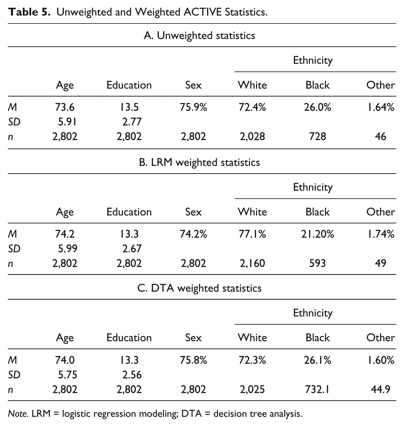
Note. LRM = logistic regression modeling; DTA = decision tree analysis.

The demographic statistics in Table 5 were then tested for equivalence with a Repeated Measures MANOVA testing weighted and unweighted values of age, education, and sex for equality. The means of these variables were significantly different in an overall test for equality (Wilks’s Lambda = 0.251, F_15,2787 = 553, p < .001), indicating that these sampling weights are not equivalent.

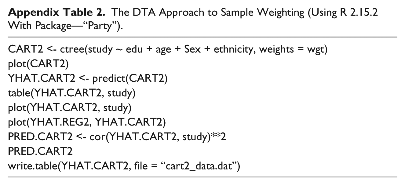
These sets of sampling weights are compared directly in Figure 2. The figure portrays the distributions of each of the weighting methods. Each method differs in implementation, but values tend to cluster around 1, for no change in person weighting. The LRM, DTA, and post-stratification methods provide peaked distributions, whereas the raking method has a relatively flat distribution.

Figure 2.

Scatterplot of DTA determined weights as a function of LRM determined weights.

Results of MANOVA Analyses: Weighted Versus Unweighted

The weights did not change the patterns of means (results available from authors), except for minor variations in explained variance.

Discussion

A few statistically significant differences between the original ACTIVE sample and the more nationally representative weighted HRS sample were identified. The ACTIVE sample was slightly younger, more educated, more female, and included more Blacks than the HRS sample. However, we should point out that the statistical models used here (LRM and DTA) have already proven that they can pick up substantial sampling biases (see McArdle, 2013), and that is not really the case here. In essence, the ACTIVE participants are very much like the HRS participants when we only consider their ages, the level of their educational attainments, their sex, and their race/ethnicity (i.e., only between 8.4% and 14.6% different).

The sampling weights we created show some changes to the demographic factors, with modifications mainly to sex and race/ethnicity breakdowns. The 2000 Current Population Survey (CPS) provides estimates of the U.S. population make up on these variables. The average age of individuals over 65 years old was 74.5 years, with males being 42.4% and females 57.6% of the population. The breakdown of race indicated that in 2000, 88.5% of the U.S. population was White, 8.4% was Black, and 3.1% was of another race (Asian, Pacific Islander, Native American). The educational attainment of the selected group of older adults was measured to be 12.5 years of education. These point to an oversampling of females and individuals with higher levels of education in the HRS, and now in ACTIVE as well. The lack of a full realization of the White subgroup (back to 88.5%) is a dramatic effect of the sampling approaches used in these studies. Again, in the ACTIVE Study, this was a direct result of the deliberate attempts to enroll Black participants.

The inclusion of indicators used in the current study identifies major person characteristics that each study should have within their data set. These data could be expanded in future studies to accommodate more characteristics about persons to make sure that they are unbiased. Such characteristics as vision, driving habits, and general mobility may be important aspects of a study question, and it would make sense to reweigh the ACTIVE sample if these are important baseline characteristics. As a starting point for examining the national representativeness of ACTIVE, this first look provides good support for a sample that can be compared with the national population.

In conclusion, we have created four sets of sampling weights for each person (labeled LRM, DTA, post-stratification, and raking) that can now be applied to any subsequent analysis of ACTIVE data. Although we have not created Inverse Mills ratios that could be used in a “Heckman” type regression correction, the same concepts are used here (see Puhani, 2000).

The choice between sampling weights is a choice that must be made by the researcher (and see Stapleton, 2002). Nevertheless, if any of these sampling weights are used in subsequent analyses, the ACTIVE sample can then be said to be nationally representative, or at least as nationally representative as the HRS sample, and this seems a definite advantage. However, given the small range of sociodemographic differences between the ACTIVE and HRS samples noted above and the lack of bias from sampling techniques, the use of sample weights in an analysis of intervention effects would not change the pattern of reported outcomes through 5 years post-intervention—that is, results through 5 years reported by the ACTIVE investigators can be considered generalizable to the U.S. population.

Footnotes

Appendix

Appendix Table 2.

The DTA Approach to Sample Weighting (Using R 2.15.2 With Package—“Party”).

CART2 <- ctree(study ~ edu + age + Sex + ethnicity, weights = wgt)

plot(CART2)

YHAT.CART2 <- predict(CART2)

table(YHAT.CART2, study)

plot(YHAT.CART2, study)

plot(YHAT.REG2, YHAT.CART2)

PRED.CART2 <- cor(YHAT.CART2, study)**2

PRED.CART2

write.table(YHAT.CART2, file = “cart2_data.dat”)

Acknowledgements

The authors thank Dr. Sharon Tennstedt from NERI for her constant concerns and continuing oversight of this project.

Authors’ Note

The content of this article is solely the responsibility of the authors and does not necessarily represent the official views of the National Institute of Nursing Research, National Institute on Aging, or the National Institutes of Health. Representatives of the funding agency have been involved in the review of the manuscript but not directly involved in the collection, management, analysis, or interpretation of the data. Dr. McArdle was a member of the Data and Safety Monitoring Board of the ACTIVE Study from 1995 to 2000 but has never had financial gains from this study.

Declaration of Conflicting Interests

The authors declared no potential conflicts of interest with respect to the research, authorship, and/or publication of this article.

Funding

The authors disclosed receipt of the following financial support for the research, authorship, and/or publication of this article: This research was conducted under Grant U01AG014282 from the National Institute on Aging to the New England Research Institutes (NERI). ACTIVE is supported by grants from the National Institute on Aging and the National Institute of Nursing Research to Hebrew Senior Life (U01NR04507), Indiana University School of Medicine (U01NR04508), Johns Hopkins University (U01AG14260), New England Research Institutes (U01AG14282), Pennsylvania State University (U01AG14263), University of Alabama at Birmingham (U01AG14289), University of Florida (U01AG14276).

References

Ball

Berch

D. B.

Helmers

K. F.

Jobe

J. B.

Leveck

M. D.

Marsiske Willis

S. L.

(2002). Effects of cognitive training interventions with older adults: A randomized controlled trial. Journal of the American Medical Association, 288, 2271-2281.

Breiman

Friedman

Olshen

Stone

(1984). Classification and regression trees. Pacific Grove, CA: Wadsworth and Brooks/Cole.

Cole

S. R.

Hernan

M. A.

(2008). Constructing inverse probability weights for marginal structural models. American Journal of Epidemiology, 168, 656-664.

Deville

J. C.

Sarndal

C. E.

Sautory

(1993). Generalized raking procedures in survey sampling. Journal of the American Statistical Association, 88, 1013-1020.

Hauser

R. M.

Willis

R. J.

(2005). Survey design and methodology in the health and retirement study and the Wisconsin longitudinal study. In Waite

L. J.

(Ed.), Aging, health, and public policy: Demographic and economic perspectives (pp. 209-235). New York, NY: Population Council.

Holt

Smith

T. M. F.

(1979). Post stratification. Journal of the Royal Statistical Society. Series A, 142, 33-46.

Horn

J. L.

(1967). On subjectivity in factor analysis. Educational and Psychological Measurement, 27, 811-820.

Hosmer

D. W.

Lemeshow

(1989). Applied logistic regression. New York, NY: Wiley.

Hothorn

Hornik

Zeileis

(2006). Unbiased recursive partitioning: A conditional inference framework. Journal of Computational and Graphical Statistics, 17, 492-514.

10.

Jobe

J. B.

Smith

D. M.

Ball

Tennstedt

S. L.

Marsiske

Willis

S. L.

Kleinman

(2001). ACTIVE: A cognitive intervention trial to promote independence in older adults. Controlled Clinical Trials, 22, 453-479.

11.

Juster

Suzman

(1995). Overview of the health and retirement study. Journal of Human Resources, 30, S7-56.

12.

Kaufman

A. S.

Kaufman

J. C.

Liu

Johnson

C. K.

(2009). How do educational attainment and gender relate to fluid intelligence, crystallized intelligence, and academic skills at ages 22-90 years? Archives of Clinical Neuropsychology, 24, 153-163.

13.

Kish

(1995). Methods for design effects. Journal of Official Statistics, 11, 55-77.

14.

Little

R. J. A.

(1993). Post-stratification: A modeler’s perspective. Journal of the American Statistical Association, 88, 1001-1012.

15.

McArdle

J. J.

(2011). Exploratory data mining using CART in the behavioral science. In Cooper

Panter

(Eds.), Handbook of methodology in the behavioral sciences (pp. 405-421). Washington, DC: APA Books.

16.

McArdle

J. J.

(2013). Dealing with longitudinal attrition using logistic regression and decision tree analyses. In McArdle

J. J.

Ritschard

(Eds.), Contemporary issues in exploratory data mining in the behavioral sciences (pp. 282-311). New York, NY: Taylor & Francis.

17.

McArdle

J. J.

Ferrer-Caja

Hamagami

Woodcock

R. W.

(2002). Comparative longitudinal structural analyses of the growth and decline of multiple intellectual abilities over the life span. Developmental Psychology, 38, 115-142.

18.

McArdle

J. J.

Fisher

G. G.

Kadlec

K. M.

(2007). Latent variable analyses of age trends of cognition in the Health and Retirement Study, 1992-2004. Psychology and Aging, 22, 525-545.

19.

McArdle

J. J.

Hamagami

(1994). Logit and multilevel logit modeling studies of college graduation for 1984-85 freshman student athletes. Journal of American Statistical Association, 89, 1107-1123.

20.

McArdle

J. J.

Prindle

J. J.

(2008). A latent change score analysis of a randomized clinical trial in reasoning training. Psychology and Aging, 23, 702-719.

21.

Puhani

P. A.

(2000). The Heckman correction for sample selection and its critique. Journal of Economic Surveys, 14, 53-68.

22.

R Core Team. (2013). R: A language and environment for statistical computing (ISBN 3-900051-07-0). Vienna, Austria: R Foundation for Statistical Computing. Available from http://www.R-project.org/

23.

Rebok

G. W.

Carlson

M. C.

Langbaum

J. B.

(2007). Training and maintaining memory abilities in healthy older adults: Traditional and novel approaches. Journals of Gerontology. Series B, Psychological Sciences and Social Sciences, 62(Spec. No. 1), 53-61.

24.

Schaie

K. W.

Willis

S. L.

(1993). Age difference patterns of psychometric intelligence in adulthood: Generalizability within and across ability domains. Psychology and Aging, 8, 44-55.

25.

Stapleton

L. M.

(2002). The incorporation of sample weights into multilevel structural equation models. Structural Equation Modeling, 9, 475-502.

26.

Strobl

Malley

Tutz

(2009). An introduction to recursive partitioning: Rationale, application, and characteristics of classification and regression trees, bagging, and random forests. Psychological Methods, 14, 323-348.

27.

Therneau

Atkinson

Ripley

(2012). rpart: Recursive partitioning (R package version 4.1-0).

28.

Willis

S. L.

Tennstedt

S. L.

Marsiske

Ball

Elias

Koepke

K. M.

Wrignt

(2006). Long-term effects of cognitive training on everyday functional outcomes in older adults. Journal of the American Medical Association, 296, 2805-2814.

29.

Zimprich

Martin

(2002). Can longitudinal changes in processing speed explain longitudinal age changes in fluid intelligence? Psychology and Aging, 17, 690-695.