Infinite Boundary Value Problems for the p -Laplacian with Nonlinear Gradient Terms

Abstract

In this paper, we investigate the existence/non-existence, exact asymptotic behavior at the boundary and uniqueness of solutions to infinite boundary-value problems of the $p$ -Laplace equation with lower-order nonlinear gradient terms in bounded open subsets of $R^{n}$ . The main tool is a recently obtained comparison principle, that captures the subtlety that arises due to the presence of the nonlinear gradient term. To the best of our knowledge, the results contained herein are comprehensive and cover topics that have not been addressed in the literature, except for very special cases.

1. Introduction

Let $Ω \subseteq R^{n}$ be a bounded open set, and $p > 1$ a fixed constant. Consider a continuous function $H : R \times R_{0}^{+} \to R$ , where $R_{0}^{+} := [0, \infty)$ . A function $u \in W_{l o c}^{1, p} (Ω)$ is said to be a subsolution (respectively, supersolution) of

Δ_{p} u = H (u, | D u |)

(1.1)

Ω

if and only if

H (u, | D u |) \in L_{l o c}^{1} (Ω)

, and

- \int_{Ω} | D u |^{p - 2} D u \cdot D ϕ \geq (resp . \leq) \int_{Ω} H (u, | D u |) ϕ, \forall ϕ \in C_{c}^{1} (Ω), ϕ \geq 0 in Ω .

We say

u \in W_{l o c}^{1, p} (Ω)

is a solution of (1.1) provided

u

is a subsolution (written

Δ_{p} u \geq H (u, | D u |)

) of (1.1) and is a supersolution (written

Δ_{p} u \leq H (u, | D u |)

) of (1.1) in

Ω

. In other words,

u \in W_{l o c}^{1, p} (Ω)

is a solution of (1.1) if and only if

- \int_{Ω} | D u |^{p - 2} D u \cdot D ϕ = \int_{Ω} H (u, | D u |) ϕ \forall ϕ \in C_{c}^{1} (Ω) in Ω .

We remark that if $u \in W^{1, \infty} (Ω)$ , then a simple density argument shows that we can take $ϕ \in W_{0}^{1, p} (Ω)$ as a test function in the above definitions.

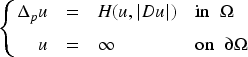
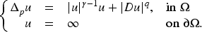
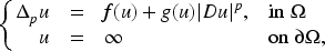
Our primary objective in this paper is the investigation of the following infinite boundary-value problem for given continuous functions $f, g : R \to R$ , and given parameters $p > 1$ and $q > 0$ .

{\begin{cases} Δ_{p} u = f (u) + g (u) | D u |^{q} & in Ω \\ u = \infty & on \partial Ω . \end{cases}

($\boldsymbol{\mathcal{A}^+}$)

Here, by a solution to (

A^{+}

) we mean a function

u \in W_{l o c}^{1, p} (Ω) \cap C (Ω)

that solves (1.1) in

Ω

, with

H (s, t) := f (s) + g (s) t^{q}

, and satisfies

u (x) \to \infty

x \to \partial Ω

. Such solutions are known in the literature as large solutions or boundary blow-up solutions. We will use a similar definition of the boundary blow-up solution when the right-hand side term of the PDE in

(A^{+})

is replaced by any general term

H (u, | D u |)

Infinite boundary-value problems have their roots in mathematical physics and Riemannian geometry (see Bieberbach 1916; Rademacher 1943). In fact, the first such application goes all the way back to 1916 when Bieberbach in Bieberbach (1916) sought to find a large solution of $Δ u = κ \exp (2 u), κ > 0,$ in a bounded smooth planar domain $Ω$ in order for $| d s |^{2} = \exp (2 u (x)) | d x |^{2}$ to define a complete Riemannian metric on $Ω$ with Gaussian curvature $- κ$ . Several decades later, and motivated by a problem in mathematical physics, Rademacher studied in Rademacher (1943) a similar problem in a bounded smooth domain $Ω \subset R^{3}$ . It was not until the works of J.B. Keller in Keller (1957) and R. Osserman in Osserman (1957) that interest in infinite boundary-value problems garnered widespread interest. In 1957, these authors independently studied large solutions of $Δ u = f (u)$ in bounded smooth domains $Ω \subset R^{n}$ . They provided necessary and sufficient conditions on $f$ in order for the aforementioned equation to have a large solution in $Ω$ . To wit, let $f : R \to R$ be a non-decreasing continuous function such that $f (0) = 0$ and $f (t) > 0$ for $t > 0$ . Keller and Osserman showed that $Δ u = f (u)$ admits a solution in $Ω$ if and only if

\int_{1}^{\infty} \frac{d t}{\sqrt{F (t)}} < \infty,

(1.2)

where

F

is the antiderivative of

f

that vanishes at zero. For instance, when

f (t) := | t |^{γ - 1} t

the problem admits a solution in a

Ω

if and only if

γ > 1

The literature on boundary blow-up problems is extensive, and it is impossible to give an exhaustive list. In this paper, we will only mention works that are closely aligned with our work and that served as motivation to our investigation in this paper.

Problem $(A^{+})$ has been studied widely when $g \equiv 0$ . Let us mention a few works in this regard. In the paper Díaz and Letelier (1993), G. Diaz and R. Letelier, among many other results, show the existence of solutions to ( $A^{+}$ ) when $f (t) = t^{γ}$ for $γ > p$ and $g \equiv 0$ . Similarly, J. Matero in Matero (1996) and F. Gladiali and G. Porru in Gladiali and Porru (1998) show that Problem ( $A^{+}$ ), with $g \equiv 0$ , has a solution for a nonlinearity $f$ where $f : R \to [0, \infty)$ is a non-decreasing continuous function provided that (i) of (2.1), given below, holds.

Of course, condition (2.1), (i) is a generalization of the Keller–Osserman growth condition (1.2) adapted to Problem ( $A^{+}$ ) for $p \neq 2$ . For investigations of large solutions that focus on quasilinear equations we refer to Díaz and Letelier (1993), Du (2003), Du (2004), Du and Guo (2003), Ghergu and Radulescu (1997), Gladiali and Porru (1998), Karls and Mohammed (2016), Lair and Mohammed (2023), Leonori and Porretta (2016), Lieberman (2011), Mohammed (2007), Mohammed (2010), Zhang (2017) and Zhang and Kan (2023). Problem $(A^{+})$ for the case $p = q = 2$ was studied in Porretta (2004).

In sharp contrast to the type of problems mentioned above, Problem ( $A^{+}$ ) with $g ≢ 0$ is vastly different and involves some subtleties. The nonlinear lower gradient term in Problem ( $A^{+}$ ) introduces additional complexities that require careful analysis. In the case $p = 2$ , such problems appear in stochastic control theory and were studied by Lasry and Lions (1989), with $g \equiv 1$ , but with $λ u + a (x),$ in place of $f (u)$ . Here $λ > 0$ is a constant, and $a \in C^{1} (Ω)$ . In Bandle and Giarrusso (1996), C. Bandle and E. Giarrusso investigated existence and asymptotic boundary behavior to Problem ( $A^{+}$ ) with $f (t) = e^{t}, (f (t) = t^{m})$ and $g (t) = \pm 1$ . See also Bandle and Essen (1994).

The recent paper (Lair & Mohammed, 2023) investigates the existence and non-existence of solutions to Problem ( $A^{+}$ ) for the $p = 2$ case. We refer to the works (Zhang, 2006, 2014) of Z. Zhang for discussion on existence and asymptotic boundary behavior of large solutions to Problem $(A^{+})$ for the case $p = 2$ . In fact, Zhang (2014) studies large solutions of $Δ u = a (x) f (u) + b (x) g (u) | D u |^{q}, q \in (0, 2]$ , when $a$ and $b$ are Hölder continuous on $\bar{Ω}$ , positive in $Ω$ , but are allowed to vanish on the boundary. In the papers Cîrstea and Rădulescu (2006, 2007), Cîrstea and Rădulescu pioneered the use of Karamata theory to study sharp boundary asymptotic behavior of solutions for equations of the form ( $A^{+}$ ) for the $p = 2$ case in the absence of gradient terms.

The work on Problem ( $A^{+}$ ) for the $p$ -Laplacian case is sparse, at least to the best of our knowledge. The lack of a comprehensive study in the literature of Problem $(A^{+})$ for general $p > 1, q > 0$ can perhaps be explained by the fact that suitable comparison principle that can be used in analyzing the problem has been missing. Recently, A. Vitolo and one of the authors of the paper have studied in Mohammed and Vitolo (2024a, 2024b) comparison principles for solutions to the PDE in $(A^{+})$ , and with the aid of these newly availed tools, we are now able to make complete investigation into Problem $(A^{+})$ .

Large solutions have also been studied when the principal parts are fully non-linear. For instance, see Alarcón and Quaas (2013), Chen et al. (2015), Mohammed and Vitolo (2019), Mohammed et al. (2020), Zhang and Du (2018), Zhang and Feng (2019).

As already noted in the works of Bandle and Giarrusso (1996) for the case $p = 2$ , the boundary blow-up problem for the equation $Δ_{p} u = f (u) - g (u) | D u |^{q}$ exhibits a drastically different behavior and new type of growth conditions on $f$ and $g$ are needed. This will the subject of a forthcoming work.

2. Basic Assumptions

For easy reference, in this section we collect all the basic assumptions used in this paper. Unless specified differently, $Ω$ will always denote a bounded open subset of $R^{n}$ with $C^{1, α}$ boundary for some $0 < α \leq 1$ . Let us mention from the outset that throughout, $f, g : R \to R$ are always assumed to be continuous. Also in this paper, we will say $h$ is non-decreasing (respectively, increasing) on a non-empty subset $J \subseteq R$ to mean that $h (t_{1}) \leq h (t_{2})$ (respectively, $h (t_{1}) < h (t_{2})$ ) whenever $t_{1}, t_{2} \in J$ and $t_{1} < t_{2}$ . A similar definition is used for non-increasing or decreasing.

We begin with conditions on $f, g$ that we will use for some of our main results. Problem $(A^{+})$ has been explored extensively when $g \equiv 0$ . For instance, see the papers (Díaz & Letelier, 1993; Du, 2003, 2004; Du & Guo, 2003; Gladiali & Porru, 1998; Matero, 1996; Mohammed, 2007, 2010). In view of this, in this paper we only consider the case $g ≢ 0$ .

The following conditions on $f$ and $g$ , stated vis-à-vis the relative ranges of $p > 1, q > 0$ , will allow us to use comparison principles to investigate Problem ( $A^{+}$ ).

(A-1) $^{+}$ :
Let $f, g : R \to R$ be non-decreasing, and furthermore assume one of the following is true. (i)
$f$ is increasing when $p \geq 2, q > 0$ , and when $1 < p < 2, 0 < q < 1$ .
(ii)
$g$ is increasing when $p \geq 2, q \geq 1$ , $f$ is increasing when $p \geq 2, 1 \leq q \leq p - 1$ , and when $p > 1, 0 < q \leq 1$ .

Note that in (i) of (A-1) $^{+}$ , we only demand that $f$ and $g$ are non-decreasing (and of course, continuous as well) when $1 < p < 2$ , and $q \geq 1$ .

Next, we consider conditions on $f$ and $g$ that are needed to study Problem $(A^{+})$ when $0 < q < p$ .

The following Keller–Osserman type condition on $f$ and $g$ , non-negative on $R_{0}^{+}$ , will play a crucial role in the investigation of $(A^{+})$ .

$(K O)_{q < p}^{+}$ :
$\int_{1}^{\infty} \frac{d s}{F {(s)}^{\frac{1}{p}} + G {(s)}^{\frac{1}{p - q}}} < \infty .$
Here, $F$ and $G$ are the antiderivatives of $f$ and $g$ , respectively, that vanish at zero.

It is clear that when $0 < q < p$ , $(K O)_{q < p}^{+}$ holds if either of the following is true.
$(i) \int_{1}^{\infty} \frac{d s}{F {(s)}^{\frac{1}{p}}} < \infty, (i i) \int_{1}^{\infty} \frac{d s}{G {(s)}^{\frac{1}{p - q}}} < \infty .$
(2.1)
It is convenient to refer to (i) of (2.1) as the $p$ -Keller–Osserman condition, and (ii) of (2.1) as the $(p - q)$ -Keller–Osserman condition. We wish to point out that if $g$ is non-decreasing, $g (τ) > 0$ for some $τ > 0$ , and $p - 1 < q < p$ , then the $(p - q)$ -Keller–Osserman condition, and hence $(K O)_{q < p}^{+}$ , holds.

We will use the following condition to show existence of solution to $(A^{+})$ when $p = q$ . $(K O)_{q = p}^{+}$ :
$\int_{a}^{\infty} {(\int_{a}^{t} \exp (\frac{p}{n (p - 1)} \int_{s}^{t} g (τ) d τ) f (s) d s)}^{- \frac{1}{p}} d t < \infty for a > 0$ .
Obviously, $(K O)_{p = q}^{+}$ holds when the $p$ -Keller–Osserman condition holds. It also holds provided that $f$ and $g$ are non-decreasing and $f (t) > 0, g (t) > 0$ for all $t > 0$ . See the discussion at the end of Section 4.
Remark 2.1
It will be convenient to adopt the following convention. We will simply say $(K O)_{q}^{+}$ holds when $(K O)_{q < p}^{+}$ holds for $0 < q < p$ , and when $(K O)_{q = p}^{+}$ holds for $q = p$ .

The uniform local boundedness of solutions to (1.1) is a crucial result in the proof the existence of a solution to Problem $(A^{+})$ . However, to achieve this we will need the following limits: (i)
$lim_{a \to \infty} \int_{a}^{\infty} \frac{d s}{F (s, a)^{\frac{1}{p}} + G (s, a)^{\frac{1}{p - q}}} = 0, when 0 < q < p,$
(ii)
$lim_{a \to \infty} \int_{a}^{\infty} {(\int_{a}^{t} \exp (\frac{p}{n (p - 1)} \int_{s}^{t} g (τ) d τ) f (s) d s)}^{- \frac{1}{p}} d t = 0, when q = p .$
See (4.2) in Section 4 for the notations $F$ and $G$ . The limit in (i) follows from condition $(K O)_{q < p}^{+}$ when $0 < q \leq p - 1$ . However $(K O)_{q}^{+}$ is not sufficient for the limit (i), when $p - 1 < q < p$ or for the limit (ii), when $q = p$ . Therefore, we need the following additional condition when $p - 1 < q \leq p$ to ensure that these limits hold.
$\begin{aligned} (L-I): lim_{t \to \infty} f (t) = \infty or lim_{t \to \infty} g (t) = \infty . \end{aligned}$
We would like to emphasize that whenever condition (L-I) is invoked, we always assume that $p - 1 < q \leq p$ .

We refer to the paper Bhattacharya and Mohammed (2021, Appendix B) to see that (L-I) and $(K O)_{q < p}^{+}$ together imply the limit in (i). Later in Section 4 we will verify that (L-I) and $(K O)_{q = p}^{+}$ are sufficient for the limit in (ii).

In our investigation of boundary asymptotic estimates for solutions of $(A^{+})$ for the case $0 < q < p$ , the class of rapidly varying functions, which we now recall, will play a crucial role. We will say that a function $h$ is regularly varying (at infinity) of index $ρ \in R$ , written $h \in R V_{ρ}$ , if $h$ is a positive measurable function on $[a, \infty)$ for some $a > 0$ and if
$lim_{t \to \infty} \frac{h (A t)}{h (t)} = A^{ρ} for all constants A > 0.$

We will also use the following conditions to study uniqueness of solutions to $(A^{+})$ . ( $N-D$ ):
$t \mapsto \frac{f (t)}{t^{p - 1}}$ , and $t \mapsto \frac{g (t)}{t^{p - q - 1}}$ are non-decreasing in $R^{+}$ .

Remark 2.2
If $f \in R V_{σ}$ for some $σ > p - 1$ , then (i) of (2.1) holds. Similarly if $g \in R V_{κ}$ for some $κ > p - q - 1$ , then (ii) of (2.1) holds. See Appendix B for proof of these assertions. In such cases, we will use $Φ_{f}$ and $Φ_{g}$ to denote the functions determined by the following relations for all $t > 0$ .
$(I) \int_{Φ_{f} (t)}^{\infty} \frac{d s}{F {(s)}^{\frac{1}{p}}} = t, and (I I) \int_{Φ_{g} (t)}^{\infty} \frac{d s}{G {(s)}^{\frac{1}{p - q}}} = t .$
(2.2)

Note that $Φ_{f} (t) \to \infty$ and $Φ_{g} (t) \to \infty$ as $t \to 0^{+}$ . We also remark that, when $p - 1 < q \leq p$ the condition (N-D) is strictly weaker than requiring $g$ to be non-decreasing. Of course, when $q = p - 1$ , the condition merely states that $g$ is non-decreasing.

When $p = q$ , and assuming that condition $(K O)_{q = p}^{+}$ holds, we will define $Φ$ by the relationship:
$\int_{Φ (r)}^{\infty} {(\frac{p}{p - 1} \int_{0}^{t} \exp (\frac{p}{p - 1} \int_{s}^{t} g (τ) d τ) f (s) d s)}^{- 1 / p} d t = r, \forall r > 0.$
(2.3)
3. Main Results

In this section, we collect the main results of the paper. Our first result gives a necessary and sufficient condition for the existence of solutions to Problem $(A^{+})$ for the case $0 < q \leq p$ . At this point, we would like to draw the reader’s attention to the convention we have adopted in Remark 2.1.

Theorem 3.1 Existence

Assume that (A-1) $^{+}$ and (L-I) hold, $f (t) > 0, g (t) \geq 0$ for $t > 0$ , and $f (0) = 0$ . If $(K O)_{q}^{+}$ holds, then Problem $(A^{+})$ admits a solution in $W_{l o c}^{1, \infty} (Ω)$ .

Our first non-existence result as follows.

Theorem 3.2 Non-existence for the case $0 < q \leq p$

Assume that condition (A-1) $^{+}$ holds. Then Problem $(A^{+})$ has no non-negative solution in $W_{l o c}^{1, \infty} (Ω)$ under either of the following conditions.

(i)
$f (t) > 0, g (t) \geq 0$ for $t > 0$ , $f (0) = 0$ , and $(K O)_{q < p}^{+}$ fails.
(ii)
$p \geq 2, p - 1 < q \leq p$ , $f \equiv 0$ and $g \geq 0$ is non-decreasing. When $q = p - 1$ , we assume that $g$ is increasing.

Remark 3.3
Assume that the assumptions of Theorem 3.2 hold. Then Problem $(A^{+})$ has no non-negative solution in $W_{l o c}^{1, p} (Ω) \cap L_{l o c}^{\infty} (Ω)$ . If such a solution $u$ were to exist, then Lieberman (1991, Theorem 1.7) would imply that $u \in W_{l o c}^{1, \infty} (Ω)$ , which is not possible by Theorem 3.2.

The next result shows that Problem $(A^{+})$ has no non-negative solution if $q > p$ .
Theorem 3.4 Non-existence for the case $q > p$

Let $Ω \subseteq R^{n}$ be a bounded $C^{1}$ open set with an interior ball condition. Suppose that $f$ and $g$ satisfy condition (A-1) $^{+}$ , with $f (t) > 0$ for $t > 0, f (0) = 0$ and $g (0) > 0$ . If, in addition, $f (t) \to \infty$ as $t \to \infty$ , and $q > p$ , then Problem $(A^{+})$ has no non-negative solution in $W_{l o c}^{1, \infty} (Ω)$ .

The following gives us the asymptotic boundary behavior of solutions of $(A^{+})$ for a wide class of functions $f$ and $g$ , and when $0 < q < p$ . In its statement, we use the notation $d_{Ω} (x)$ for the distance of $x \in Ω$ to the boundary $\partial Ω$ .

Theorem 3.5 Boundary Asymptotic Estimates for the case $0 < q < p$

Let $Ω \subseteq R^{n}$ be a bounded domain with $C^{2}$ boundary $\partial Ω$ , and let $0 < q < p$ . Assume that condition (A-1) $^{+}$ holds for $f,$ and $g$ . Moreover, suppose that $f \in R V_{σ}$ for some $σ > p - 1$ , and $g \in R V_{κ}$ for some $κ > p - 1 - q$ . Then for any solution $u \in W_{l o c}^{1, \infty} (Ω)$ of $(A^{+})$ we have

\begin{aligned} lim_{d_{Ω} (x) \to 0^{+}} \frac{u (x)}{Φ_{f} (d_{Ω} (x))} = {(\frac{p - 1}{p})}^{\frac{1}{σ - (p - 1)}}, i f 0 < q < p, and \frac{σ - κ}{σ + 1} > \frac{q}{p}, \end{aligned}

(3.1)

\begin{aligned} lim_{d_{Ω} (x) \to 0^{+}} \frac{u (x)}{Φ_{g} (d_{Ω} (x))} = {(\frac{p - 1}{p - q})}^{\frac{1}{κ - (p - 1 - q)}}, i f 0 < q < p, and \frac{σ - κ}{σ + 1} < \frac{q}{p} . \end{aligned}

(3.2)

When $q = p$ , the following theorem gives the asymptotic boundary behavior of solutions to Problem $(A^{+})$ .

Theorem 3.6 Boundary Asymptotic Estimate for the case

q = p

Let $Ω \subseteq R^{n}$ be a bounded domain with $C^{2}$ boundary $\partial Ω$ , and $q = p$ . Suppose that $f$ and $g$ satisfy condition (A-1) $^{+}$ , and that $(K O)_{q = p}^{+}$ holds. Furthermore, assume that $f \in R V_{σ}$ , and $g \in R V_{κ}$ for some $σ, κ \in R_{0}^{+} .$ Then, for any solution $u \in W_{l o c}^{1, \infty} (Ω)$ of $(A^{+})$ , we have

lim_{d_{Ω} (x) \to 0^{+}} \frac{u (x)}{Φ (d_{Ω} (x))} = 1,

where

Φ

is as defined in (2.3).

As consequences of Theorem 3.5, and Theorem 3.6 we obtain our main result on uniqueness of non-negative solutions to Problem $(A^{+})$ .

Theorem 3.7 Uniqueness

Let $Ω \subseteq R^{n}$ be a bounded domain with $C^{2}$ boundary $\partial Ω$ . Let $f, g$ satisfy conditions (A-1) $^{+}$ , and (N-D)¹. For $0 < q < p$ , we assume that $f \in R V_{σ}$ , with $σ > p - 1$ , and $g \in R V_{κ}$ , with $κ > p - q - 1$ . If $(σ - κ) / (σ + 1) \neq q / p$ , then Problem $(A^{+})$ admits at most one non-negative solution in the class $W_{l o c}^{1, \infty} (Ω)$ . On the other hand, for $q = p$ , we assume that $(K O)_{q = p}^{+}$ holds, that $f \in R V_{σ}$ and $g \in R V_{κ}$ for some $σ, κ \in R_{0}^{+} .$ Then Problem $(A^{+})$ admits at most one non-negative solution in the class $W_{l o c}^{1, \infty} (Ω)$ .

4. Preliminaries and Auxiliary Results

A crucial tool we need in studying Problem ( $A^{+}$ ) is the comparison principle. Since a significant portion of this work focuses on Problem ( $A^{+}$ ), let us highlight a comparison principle from Mohammed and Vitolo (2024a, Theorem 1.3, Theorem 1.4) and Mohammed and Vitolo (2024b, Theorem 1.3, Theorem 1.4) that is strictly relevant for our purpose in this paper.

Theorem A Comparison Principle

Let $Ω \subset R^{n}$ be a bounded open set, $p > 1, q > 0$ and let $f, g : R \to R$ satisfy condition (A-1) $^{+}$ . Suppose $u, v \in W_{l o c}^{1, \infty} (Ω)$ such that

- Δ_{p} u + f (u) + g (u) | D u |^{q} \leq - Δ_{p} v + f (v) + g (v) | D v |^{q} in Ω .

If $u \leq v$ on² $\partial Ω$ , then $u \leq v$ in $Ω$ .

Our investigation of Problem ( $A^{+}$ ) is intimately related to an initial-value problem (IVP) of the following kind, where $a > 0$ is any given constant.

{\begin{array}{rcll} r^{1 - n} {(r^{n - 1} | ϕ^{'} (r) |^{p - 2} ϕ^{'} (r))}^{'} & = & H (ϕ (r), | ϕ^{'} (r) |), 0 \leq r < R, \\ ϕ (0) & = & a, ϕ^{'} (0) = 0. \end{array}

(${\bf IVP}(\textit{a})$)

Concerning existence of a solution to ( ) we require that

H : R \times R_{0}^{+} \to R

is a continuous function that satisfies the following.

(H-1):

$s \mapsto H (s, t)$ is non-decreasing in $R$ for each $t > 0$ .

(H-2):

$H (s, 0) > 0$ for $s > 0$ .

Under the assumptions (H-1) and (H-2) on $H$ given above, Problem ( ) admits a solution $ϕ \in C^{2} ((0, R)) \cap C^{1} ([0, R))$ , for some $0 < R \leq \infty$ . We assume that $[0, R)$ is the maximal interval of existence of $ϕ$ . Moreover, we also have $ϕ > 0, ϕ^{'} > 0$ and $ϕ^{″} \geq 0$ in $(0, R)$ . Since we couldn’t find a suitable reference for ( ) that meets our needs, and to ensure thoroughness, we’ve opted to incorporate a comprehensive discussion of the IVP ( ) in Appendix A.

Remark 4.1

While $ϕ^{″}$ may not exist at $r = 0$ , the differential equation in ( ) holds, in the classical sense, in the open interval $(0, R)$ . Therefore $ϕ$ satisfies the equation:

(p - 1) (ϕ^{'} (r))^{p - 2} ϕ^{″} (r) + \frac{n - 1}{r} (ϕ^{'} (r))^{p - 1} = H (ϕ (r), ϕ^{'} (r)), 0 < r < R .

(4.1)

Remark 4.2

Suppose that $ϕ \in C^{2} ((0, R)) \cap C^{1} ([0, R))$ is a solution of Problem ( ). Given $z \in R^{n}$ the function

w (x) := ϕ (| x - z |), x \in B := B (z, R)

belongs³ to

W_{l o c}^{1, \infty} (B (z, R))

, and is a solution of (1.1) in

Ω := B (z, R)

For the rest of this section we focus on the IVP ( ) for a given $a > 0$ , where we take $H (s, t) = f (s) + g (s) t^{q}$ with $f, g : R \to R$ non-decreasing, continuous functions such that $f (t) > 0$ , and $g (t) \geq 0$ for $t > 0$ . Notice that in this case $H$ satisfies both conditions (H-1) and (H-2). For $p = 2$ , Problem ( $A^{+}$ ) has recently been investigated in the papers (Lair & Mohammed, 2023; Zhang, 2014).

Let us now focus on the IVP ( ) and assume that $ϕ \in C^{2} ((0, R)) \cap C^{1} ([0, R))$ is a solution of Problem ( ) on a maximal interval of existence $[0, R)$ , where $0 < R \leq \infty$ . Hereafter, it will be convenient to use the following notations.

F (t, s) := \int_{s}^{t} f (τ) d τ, and G (t, s) := \int_{s}^{t} g (τ) d τ for 0 < s \leq t .

(4.2)

Going back to (4.1), it follows that

(p - 1) (ϕ^{'} (r))^{p - 2} ϕ^{″} (r) \leq f (ϕ (r)) + g (ϕ (r)) (ϕ^{'} (r))^{q}, 0 < r < R .

(4.3)

We multiply both sides by

ϕ^{'} > 0

and integrate on

(ρ, r)

for any

0 < ρ < r < R

. We find

\frac{p - 1}{p} [(ϕ^{'} (r))^{p} - (ϕ^{'} (ρ))^{p}] \leq \int_{0}^{r} f (ϕ (t)) ϕ^{'} (t) d t + \int_{0}^{r} g (ϕ (t)) (ϕ^{'} (t))^{q + 1} d t

(4.4)

We first suppose that $0 < q < p$ .

Letting $ρ \to 0^{+}$ in (4.4), and recalling that $f$ and $g$ are non-negative on $[0, \infty)$ , we find for $ϵ > 0$

\begin{aligned} \frac{p - 1}{p} (ϕ^{'} (r))^{p} \leq \int_{0}^{r} f (ϕ (t)) ϕ^{'} (t) d t + (ϕ^{'} (r))^{q} \int_{0}^{r} g (ϕ (t)) ϕ^{'} (t) d t, since ϕ is\ convex, . \\ = F (ϕ (t)) - F (ϕ (0)) + (ϕ^{'} (r))^{q} [G (ϕ (r)) - G (ϕ (0))] \\ \leq F (ϕ (r), ϕ (0)) + ϵ (ϕ^{'} (r))^{p} + \frac{p - q}{p} {(\frac{p}{q} ϵ)}^{- q / (p - q)} G (ϕ (r), ϕ (0))^{p / (p - q)}, \end{aligned}

where, in the last inequality we have used Young’s inequality for any constant

ϵ > 0

. We choose

ϵ = (p - 1) / 2 p

, and rearrange to write

(ϕ^{'} (r))^{p} \leq C [F (ϕ (r), ϕ (0)) + G (ϕ (r), ϕ (0))^{\frac{p}{p - q}}],

(4.5)

for some positive constant

C := C (p, q)

, depending on

p

and

q

. In the sequel, we will use

C

to denote a positive constant that we allow to change from line to line, but will always depend on at most

p, q

and

n

. Taking the

p^{th}

root in (4.5) we find

ϕ^{'} (r) \leq C [F (ϕ (r), ϕ (0))^{\frac{1}{p}} + G (ϕ (r), ϕ (0))^{\frac{1}{p - q}}], 0 \leq r < R .

(4.6)

Integrating this on

(0, r)

for

0 < r < R

we find

\int_{a}^{ϕ (r)} \frac{d s}{F (s, a)^{\frac{1}{p}} + G (s, a)^{\frac{1}{p - q}}} \leq C r, 0 < r < R .

(4.7)

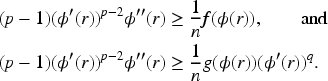
Next we estimate the integral in (4.7) from below. We begin by integrating the equation in ( ) on $(0, r)$ for $0 < r < R$ . Exploiting the convexity of $ϕ$ in $(0, R)$ we get

\begin{aligned} r^{n - 1} (ϕ^{'} (r))^{p - 1} & = \int_{0}^{r} t^{n - 1} H (ϕ (t), ϕ^{'} (t)) d t \\ \leq H (ϕ (r), ϕ^{'} (r)) \int_{0}^{r} t^{n - 1} d t \\ = \frac{r^{n}}{n} H (ϕ (r), ϕ^{'} (r)), 0 < r < R . \end{aligned}

Upon using this last inequality in (4.1) we obtain

\begin{aligned} H (ϕ (r), ϕ^{'} (r)) & = (p - 1) (ϕ^{'} (r))^{p - 2} ϕ^{″} (r) + \frac{n - 1}{r} (ϕ^{'} (r))^{p - 1} \\ \leq (p - 1) (ϕ^{'} (r))^{p - 2} ϕ^{″} (r) + \frac{n - 1}{r} [\frac{r}{n} H (ϕ (r), ϕ^{'} (r))] . \end{aligned}

That is

(p - 1) (ϕ^{'} (r))^{p - 2} ϕ^{″} (r) \geq \frac{1}{n} H (ϕ (r), ϕ^{'} (r)) = \frac{1}{n} f (ϕ (r)) + \frac{1}{n} g (ϕ (r)) (ϕ^{'} (r))^{q} .

(4.8)

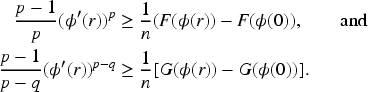
As a consequence of (4.8), the following two inequalities hold for all

0 < r < R

\begin{aligned} (p - 1) (ϕ^{'} (r))^{p - 2} ϕ^{″} (r) & \geq \frac{1}{n} f (ϕ (r)), and \\ (p - 1) (ϕ^{'} (r))^{p - 2} ϕ^{″} (r) & \geq \frac{1}{n} g (ϕ (r)) (ϕ^{'} (r))^{q} . \end{aligned}

Multiplying both sides of each inequality by

ϕ^{'}

and then integrating leads to

\begin{aligned} \frac{p - 1}{p} (ϕ^{'} (r))^{p} & \geq \frac{1}{n} (F (ϕ (r)) - F (ϕ (0)), and \\ \frac{p - 1}{p - q} (ϕ^{'} (r))^{p - q} & \geq \frac{1}{n} [G (ϕ (r)) - G (ϕ (0))] . \end{aligned}

Notice that the above two inequalities hold for

0 \leq r < R

. Thus we obtain

ϕ^{'} (r) \geq C [(F (ϕ (r)) - F (ϕ (0))^{1 / p} + (G (ϕ (r)) - G (ϕ (0))^{1 / (p - q)}] .

(4.9)

From (4.9), we obtain

C r \leq \int_{a}^{ϕ (r)} \frac{d s}{F (s, a)^{\frac{1}{p}} + G (s, a)^{\frac{1}{p - q}}}, 0 \leq r < R .

(4.10)

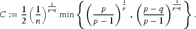
In fact, here the constant in (4.9) can be given explicitly as

C := \frac{1}{2} {(\frac{1}{n})}^{\frac{1}{p - q}} min {{(\frac{p}{p - 1})}^{\frac{1}{p}}, {(\frac{p - q}{p - 1})}^{\frac{1}{p - q}}} .

Let us now assume that

f, g : R \to R

satisfy condition (A-1)

^{+}

and also the

p

-Laplacian version of the Keller–Osserman condition

(K O)_{q}^{+}

for

0 < q < p

. Let

[0, R (a))

be the maximal interval of existence of

ϕ

. On letting

r ↑ R (a)

in (4.10), it follows that

C R (a) \leq \int_{a}^{\infty} \frac{d s}{F (s, a)^{\frac{1}{p}} + G (s, a)^{\frac{1}{p - q}}} .

(4.11)

From (4.10) we see that $R (a) \leq Ψ (a)$ , where

Ψ (a) := \frac{1}{C} \int_{a}^{\infty} \frac{d s}{F (s, a)^{\frac{1}{p}} + G (s, a)^{\frac{1}{p - q}}} .

(4.12)

On taking $α := 1 / p$ and $β := 1 / (p - q)$ for $0 < q < p$ in Bhattacharya and Mohammed (2021, Appendix B.3.1)), we obtain the following inequality.

\int_{a}^{\infty} \frac{d s}{F (s, a)^{\frac{1}{p}} + G (s, a)^{\frac{1}{p - q}}} \leq \frac{p}{p - 1} \frac{a}{F {(a)}^{\frac{1}{p}}} + 2^{\frac{1}{p - q}} \int_{2 a}^{\infty} \frac{d s}{F {(s)}^{\frac{1}{p}} + G {(s)}^{\frac{1}{p - q}}} .

(4.13)

Since we are assuming that $(K O)_{q}^{+}$ holds, where $0 < q < p$ , we see from (4.13) that $Ψ (a) < \infty$ for all $a > 0$ . We should note that $Ψ : (0, \infty) \to (0, Ψ (0 +))$ is a continuous and decreasing (strictly) function.

Also, as noted in the Appendix A, we observe that $ϕ (r) \to \infty$ as $r ↑ R (a)$ . From (4.7) we note that

Φ (a) := \int_{a}^{\infty} \frac{d s}{F {(s)}^{\frac{1}{p}} + G {(s)}^{\frac{1}{p - q}}} \leq C R (a),

(4.14)

for a positive constant

C

that depends on

p

and

q

only.

Next, we consider the case $q = p$ . We multiply both sides of (4.8), (with $q = p$ ), by

p ϕ^{'} \exp (- \frac{p}{n (p - 1)} \int_{a}^{ϕ} g (t) d t)

to obtain

{(p - 1) (ϕ^{'})^{p} \exp (- \frac{p}{n (p - 1)} \int_{a}^{ϕ} g (t) d t)}^{'} \geq \frac{p}{n} ϕ^{'} (r) f (ϕ (r)) \exp (- \frac{p}{n (p - 1)} \int_{a}^{ϕ} g (t) d t) .

Integrating this on

(0, r)

and rearranging, we find

ϕ^{'} (r) \geq {\frac{p}{n (p - 1)} \int_{a}^{ϕ (r)} \exp (\frac{p}{n (p - 1)} \int_{t}^{ϕ (r)} g (s) d s) f (t) d t}^{1 / p} .

(4.15)

Further integration of (4.15) on $(0, r)$ we obtain,

\int_{a}^{ϕ (r)} {(\int_{a}^{t} \exp (\frac{p}{n (p - 1)} \int_{s}^{t} g (τ) d τ) f (s) d s)}^{- \frac{1}{p}} d t \geq {(\frac{p}{n (p - 1)})}^{\frac{1}{p}} r .

(4.16)

Clearly, for

n > 1

and

g \geq 0

, we have

\begin{aligned} \int_{a}^{ϕ (r)} & {(\int_{a}^{t} \exp (\frac{p}{p - 1} \int_{s}^{t} g (τ) d τ) f (s) d s)}^{- \frac{1}{p}} d t \\ \leq \int_{a}^{ϕ (r)} {(\int_{a}^{t} \exp (\frac{p}{n (p - 1)} \int_{s}^{t} g (τ) d τ) f (s) d s)}^{- \frac{1}{p}} d t, 0 < r < R . \end{aligned}

Similarly, we multiply both sides of (4.3), (with $q = p$ ), by

p ϕ^{'} \exp (- \frac{p}{p - 1} \int_{a}^{ϕ} g (t) d t)

to get

{(p - 1) (ϕ^{'})^{p} \exp (- \frac{p}{p - 1} \int_{a}^{ϕ} g (t) d t)}^{'} \leq p ϕ^{'} (r) f (ϕ (r)) \exp (- \frac{p}{p - 1} \int_{a}^{ϕ} g (t) d t) .

Integrating this on

(0, r)

we find

ϕ^{'} (r) \leq {\frac{p}{p - 1} \int_{a}^{ϕ (r)} \exp (\frac{p}{p - 1} \int_{t}^{ϕ (r)} g (s) d s) f (t) d t}^{1 / p}, 0 < r < R .

(4.17)

As a consequence, for

0 \leq r < R

, we see that

\int_{a}^{ϕ (r)} {(\int_{a}^{t} \exp (\frac{p}{p - 1} \int_{s}^{t} g (τ) d τ) f (s) d s)}^{- \frac{1}{p}} d t \leq {(\frac{p}{p - 1})}^{\frac{1}{p}} r .

(4.18)

Taking the limit in (4.18) we find that $ϕ (r) \to \infty$ as $r ↑ R (a)$ (see Appendix A), we obtain the following estimate

Φ (a) := \int_{a}^{\infty} {(\int_{a}^{t} \exp (\frac{p}{p - 1} \int_{s}^{t} g (τ) d τ) f (s) d s)}^{- \frac{1}{p}} d t \leq {(\frac{p}{p - 1})}^{\frac{1}{p}} R (a),

(4.19)

where

[0, R (a))

is the maximal interval of existence of the solution

ϕ

of ( ) when

q = p

. In particular, we note that if

Φ (a) \to \infty

a \to 0^{+}

, then

R (a) \to \infty

a \to 0^{+}

We note from (4.16) that if

Ψ (a) := n^{\frac{1}{p}} \int_{a}^{\infty} {(\int_{a}^{t} \exp (\frac{p}{n (p - 1)} \int_{s}^{t} g (τ) d τ) f (s) d s)}^{- \frac{1}{p}} d t,

(4.20)

then

R (a) \leq Ψ (a), a > 0,

(4.21)

where

[0, R (a))

is the maximal interval of existence of

ϕ

in the IVP ( ), when

q = p

Finally, under condition (L-I), and (KO) $_{q = p}^{+}$ , let us show that $Ψ (a) \to 0$ as $a \to \infty$ where $Ψ$ is defined by (4.20). Let us first compute (where we will momentarily use $c$ for the positive constant $p g (a) / (n (p - 1))$ ) the following.

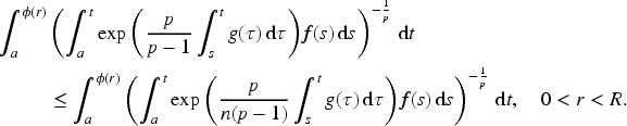
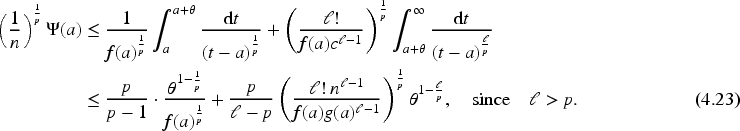
\begin{aligned} \int_{a}^{t} \exp (\frac{p}{n (p - 1)} \int_{s}^{t} g (τ) d τ) f (s) d s & \geq f (a) \int_{a}^{t} \exp (\frac{p}{n (p - 1)} g (a) (t - s)) d s \\ = \frac{f (a)}{c} [\exp (c (t - a)) - 1] \\ \geq \frac{f (a) c^{k - 1} (t - a)^{k}}{k!} \forall k = 1, 2, \dots . \end{aligned}

(4.22)

Therefore, for fixed $θ > 0$ , and an integer $ℓ > p$ we have (using $k = 1$ and $k = ℓ$ in (4.22) for the first and the last two integrals below, respectively)

\begin{aligned} {(\frac{1}{n})}^{\frac{1}{p}} Ψ (a) & \leq \frac{1}{f {(a)}^{\frac{1}{p}}} \int_{a}^{a + θ} \frac{d t}{(t - a)^{\frac{1}{p}}} + {(\frac{ℓ!}{f (a) c^{ℓ - 1}})}^{\frac{1}{p}} \int_{a + θ}^{\infty} \frac{d t}{(t - a)^{\frac{ℓ}{p}}} \\ \leq \frac{p}{p - 1} \cdot \frac{θ^{1 - \frac{1}{p}}}{f {(a)}^{\frac{1}{p}}} + \frac{p}{ℓ - p} {(\frac{ℓ! n^{ℓ - 1}}{f (a) g {(a)}^{ℓ - 1}})}^{\frac{1}{p}} θ^{1 - \frac{ℓ}{p}}, since ℓ > p . \end{aligned}

(4.23)

Let

L

be the limit of the right-hand side of the inequality in (4.23), as

a \to \infty

. Let us first assume that

g (a) \to \infty

a \to \infty

. Then, since

ℓ > p > 1

, we see that

L = (\frac{p}{p - 1}) \frac{θ^{1 - \frac{1}{p}}}{lim_{a \to \infty} f {(a)}^{\frac{1}{p}}} .

We then let

θ \to 0^{+}

to get the desired conclusion. Suppose now

f (a) \to \infty

a \to \infty

. Then we obviously find from (4.23) that

L = 0

. This concludes the proof that

Ψ (a) \to 0

a \to \infty

under the assumptions (L-I) and

(K O)_{q = p}^{+}

5. Problem

(A^{+}), 0 < q \leq p

We begin with a lemma which will provide us, under suitable assumptions on $f$ and $g$ , with uniform bound on non-negative solutions of

Δ_{p} u = f (u) + g (u) | D u |^{q} .

(5.1)

In the following lemma, we will give a uniform local bound for solutions of (5.1). In the lemma, in addition to

(K O)_{q}^{+}

, we will also assume that condition (L-I) when

p - 1 < q \leq p

. Recall that

Ψ

is defined by (4.12) in case

0 < q < p

, and is given by (4.20), when

q = p

. As a consequence of the assumptions

(K O)_{q}^{+}

and (L-I), we recall that

Ψ (a) \to 0

a \to \infty

, and hence we have

Ψ (R^{+}) = (0, Ψ (0 +)) .

Lemma 5.1

Suppose that $f$ and $g$ satisfy (A-1) $^{+}$ . Furthermore, assume that $0 < q \leq p$ and that conditions $(K O)_{q}^{+}$ and (L-I) hold. Then there is a non-increasing function $Q$ such that for any subsolution $u \in W_{l o c}^{1, p} (Ω)$ of (5.1) we have

u (x) \leq Q (d_{Ω} (x)), x \in Ω .

Proof.

As a consequence of condition $(K O)_{q}^{+}$ , and (L-I) we see that $Ψ : (0, \infty) \to (0, Ψ (0 +))$ is a well-defined decreasing function. Here $Ψ$ is as given in (4.12) when $0 < q < p$ , while $Ψ$ is as given in (4.20), when $p = q$ . As noted in (4.11), and (4.21), we recall $R (a) \leq Ψ (a)$ for any $a > 0$ . We extend the definition of the inverse function $Ψ^{- 1}$ to the interval $(0, Ψ (0 +)]$ by setting $Ψ^{- 1} (Ψ (0 +)) := 0$ . Let $u \in W_{l o c}^{1, p} (Ω)$ be any subsolution to (5.1), and fix $x \in Ω$ . First we assume that $d_{Ω} (x) < Ψ (0 +)$ , and take any $a > Ψ^{- 1} (d_{Ω} (x))$ . Let $ϕ \in C^{2} ((0, R (a)) \cap C^{1} ([0, R (a))$ be a solution to ( ), with $[0, R (a))$ as the maximal interval of existence so that $ϕ (r) \to \infty$ as $r \to R (a)$ . Then, we note that $R (a) \leq Ψ (a) < d_{Ω} (x)$ , and consequently we have the strict inclusion $B (x, R (a)) ⋐ Ω$ . We claim that $u (x) \leq a$ . To see this, let $w (y) := ϕ (| y - x |)$ , for $y \in B (x, R (a))$ . Then $w \in W_{l o c}^{1, \infty} (B)$ is a solution of $(A^{+})$ in $B := B (x, R (a))$ , and $u \leq w$ on $\partial B$ . This implies, by the comparison principle, Theorem A, that $u \leq w$ in $B$ . This would, in particular, imply that $u (x) \leq w (x) = a$ as asserted. Therefore, in this case we have shown that $u (x) \leq a$ for any $Ψ^{- 1} (d_{Ω} (x)) < a$ . In other words, we find $u (x) \leq Ψ^{- 1} (d_{Ω} (x))$ . Suppose now $Ψ (0 +) \leq d_{Ω} (x)$ . Then $Ψ (a) < d_{Ω} (x)$ for any $a > 0$ . Thus $B (x, R (a)) ⋐ Ω$ for any $a > 0$ . Arguing as in the above it would follow that $u (x) \leq a$ for all $a > 0$ so that $u (x) \leq 0 = Ψ^{- 1} (Ψ (0 +))$ .

Thus, in either case we have shown that $u (x) \leq Q (d_{Ω} (x))$ for $x \in Ω$ , where $Q (t) := Ψ^{- 1} (min {t, Ψ (0 +)}) .$

Remark 5.2

If $g \equiv 0$ , then the strict monotonicity assumption on $f$ in Lemma 5.1 can be dropped. The strict monotonicity of $f$ was needed to apply the Comparison principle, Theorem A, in the presence of the gradient term.

Proof of Theorem 3.1. Let us first suppose that $(K O)_{q}^{+}$ holds. For each positive integer $k$ , consider the Dirichlet Problem

{\begin{aligned} Δ_{p} u & = & f (u) + g (u) | D u |^{q} & in Ω; \\ u & = & k & on \partial Ω . \end{aligned}

(5.2)

Note that

v = 0

is a subsolution and

w = k

is a supersolution of (5.2). Therefore, according to Véron (2017, Corollary 1.4.5), Problem (5.2) admits a solution

u_{k} \in W^{1, p} (Ω)

such that

0 \leq u_{k} \leq k

Ω

. According to Lieberman (1988, Theorem 1), we observe that

u_{k}

belongs to

C^{1, α} (\bar{Ω})

for some

0 < α < 1

We invoke Lemma 5.1 to conclude that $0 \leq u_{k} (x) \leq Q (d_{Ω} (x))$ for $x \in Ω$ and some non-increasing function $Q$ on $R^{+}$ , independent of $k$ , and hence ${u_{k}}$ is locally uniformly bounded on $Ω$ . The Comparison Principle, Theorem A, shows that $u_{k} \leq u_{k + 1}$ in $Ω$ for all $k$ . Let $u (x) := lim_{k \to \infty} u_{k} (x)$ for $x \in Ω$ . Since ${u_{k}}$ is locally uniformly bounded in $Ω$ , we use Lieberman (1991, Theorem 1.7), and apply the Cantor diagonal argument to extract a subsequence of ${u_{k}}$ , which we will continue to denote by the same, such that $u_{k} \to u$ and $D u_{k} \to v$ uniformly on compact subsets of $Ω$ for some $v \in C (Ω)^{n}$ . In fact, it can be easily seen that $v = D u$ in the weak sense, and that $u \in C_{l o c}^{1, γ} (Ω)$ . We also note that $\underset{x \to \partial Ω}{lim inf} u \geq \underset{x \to \partial Ω}{lim inf} u_{k} = k$ , and hence $u = \infty$ on $\partial Ω$ . So it remains to show that $u$ is a solution of the PDE in Problem $(A^{+})$ . It is clear that $u$ belongs to $W_{l o c}^{1, \infty} (Ω)$ . So, let $φ \in C_{c}^{1} (Ω)$ and suppose that $O := s u p p (φ)$ . The uniform convergence of ${D u_{k}}$ and the continuity of $ξ \mapsto | ξ |^{p - 2} ξ$ on $R^{n}$ show that

lim_{k \to \infty} \int_{O} | D u_{k} |^{p - 2} D u_{k} \cdot D φ = \int_{O} | D u |^{p - 2} D u \cdot D φ .

Similarly, the uniform convergence of

{u_{k}}

and

{D u_{k}}

shows that

lim_{k \to \infty} \int_{O} (f (u_{k}) + g (u_{k}) | D u_{k} |^{q}) φ = \int_{O} (f (u) + g (u) | D u |^{q}) φ .

Therefore we conclude that

- \int_{O} | D u |^{p - 2} D u \cdot D φ = \int_{O} (f (u) + g (u) | D u |^{q}) φ \forall φ \in C_{c}^{1} (Ω) .

Proof of Theorem 3.2. By way of contradiction, suppose that $(A^{+})$ has a solution $u \in W_{l o c}^{1, \infty} (Ω)$ . Fix $x_{0} \in Ω$ and $a > max {u (x_{0}), 0}$ . Let us first suppose that (i) holds. Let $ϕ \in C^{2} ((0, R)) \cap C^{1} ([0, R))$ be a solution to ( ), where $[0, R)$ is the maximal interval of existence. Since condition $(K O)_{q < p}^{+}$ fails, we see from (4.14) that $R = \infty$ . Then $w (x) := ϕ (| x - x_{0} |)$ is a solution of (5.1) in $R^{n}$ , and thus $u \geq w$ on $\partial Ω$ . By the comparison principle we conclude that $u \geq w$ in $Ω$ . In particular, $u (x_{0}) \geq w (x_{0}) = a$ , a contradiction. On the other hand, if (ii) holds, then $w (x) \equiv a$ is a solution of (5.1), and by comparison principle, see Leonori et al. (2017, Corollary 3.1), we conclude that $w \leq u$ in $Ω$ , which again leads to a contradiction.

Corollary 5.3

Let $f, g : R \to R$ satisfy (A-1) $^{+}$ , $f (0) = 0$ , $f (t) > 0$ , and $g (t) \geq 0$ for $t > 0$ . (I)

(a)

Assume that one of the following is true:

$0 < q \leq p - 1$ ,

$p - 1 < q \leq p$ and (L-I) holds.

If $f$ satisfies the $p$ -Keller–Osserman condition, then Problem $(A^{+})$ has a non-negative solution in $W_{l o c}^{1, \infty} (Ω)$ .

(b)

Assume that one of the following is true.

$p - 1 < q < p, f (t) \to \infty$ as $t \to \infty$ , and $g (τ) > 0$ for some $τ > 0$ ,

$q = p$ , $f (t) g (t) > 0$ for $t > 0$ and (L-I) holds.

Then Problem $(A^{+})$ has a non-negative solution in $W_{l o c}^{1, \infty} (Ω)$ .

(II)

Suppose $f$ is bounded, $g (τ) > 0$ for some $τ > 0$ , and $0 < q < p$ .

If $g$ satisfies the $(p - q)$ -Keller–Osserman condition and (L-I) holds, then Problem $(A^{+})$ admits a non-negative solution in $W_{l o c}^{1, \infty} (Ω)$ .

If $g$ does not satisfy the $(p - q)$ -Keller–Osserman condition, then Problem $(A^{+})$ has no non-negative solution in $W_{l o c}^{1, \infty} (Ω)$ .

Proof.

(I)-(a): Under the given assumptions, we see that $(K O)_{q}^{+}$ and (L-I) hold. Therefore, Theorem 3.1 implies that Problem $(A^{+})$ has a non-negative solution in $W_{l o c}^{1, \infty} (Ω)$ .

(I)-(b): Let $p - 1 < q < p$ . Since $g (τ) > 0$ for some $τ > 0$ and $p - 1 < q < p$ , then (ii) of (2.1) holds. Therefore $(K O)_{q < p}^{+}$ and (L-I) are satisfied. Therefore, Theorem 3.1 applies to show that Problem $(A^{+})$ has a non-negative solution in $W_{l o c}^{1, \infty} (Ω)$ . If $q = p$ , then $(K O)_{p = q}^{+}$ holds. Hence, the claim of existence follows from Theorem 3.1.

(II): The hypotheses show that for some constants $C \geq 1, s_{0} > 0$ , we have

G {(s)}^{\frac{1}{p - q}} \leq F {(s)}^{\frac{1}{p}} + G {(s)}^{\frac{1}{p - q}} \leq C G {(s)}^{\frac{1}{p - q}} for all s \geq s_{0} .

As a consequence, the desired conclusion follows from Theorems 3.1 and 3.2.

Theorem 5.4

Assume condition (A-1) $^{+}$ . Suppose that $(K O)_{q}^{+}$ holds for $0 < q \leq p$ , and that $Φ (0 +) = \infty$ , where $Φ$ is as defined in (4.14) for $0 < q < p$ , and is given as in (4.19) when $q = p$ . Then any solution in $W_{l o c}^{1, \infty} (Ω)$ of $(A^{+})$ , if it exists, must be positive in $Ω$ .

Proof.

Let $u \in W_{l o c}^{1, \infty} (Ω)$ be a solution of $(A^{+})$ , and let us assume, if possible, that there is $z \in Ω$ such that $u (z) \leq 0$ . Let $ϕ \in C^{2} ((0, R)) \cap C^{1} ([0, R))$ be a solution to ( ) with $[0, R (a))$ as its maximal interval of existence, and where $a > 0$ is chosen such that $Ω ⋐ B (z, R (a))$ . This is possible, since (4.14) and (4.19) show that $R (a) \to \infty$ as $a \to 0^{+}$ as a result of the assumption $Φ (0^{+}) = \infty$ . Now, we recall $w (x) := ϕ (| x - z |)$ is a solution of (5.1) and $w \in W_{l o c}^{1, \infty} (Ω)$ . Therefore, $w \leq u$ on $\partial Ω$ . But, then by the Comparison Principle, Theorem A, we conclude that $w \leq u$ in $Ω$ . In particular, we see that $a = w (z) \leq u (z)$ , which is a clear contradiction.

6. Problem

(A^{+}), q > p

In this section we show that Problem $(A^{+})$ has no non-negative solution in $Ω$ if $q > p$ . In fact, we will show that the following problem

{\begin{array}{rcll} Δ_{p} u & = & H (u, | D u |) & i n Ω \\ u & = & \infty & o n \partial Ω \end{array}

($\boldsymbol{\mathcal{H}}$)

does not admit any non-negative solution under some suitable assumptions on the Hamiltonian

H

. In addition to conditions (H-1) and (H-2) we already considered on the continuous function

H : R \times R_{0}^{+} \to R_{0}^{+}

, we will also make the following assumptions.

(H-3):

$H$ is non-decreasing in each variable.

(H-4):

$\int_{1}^{\infty} \frac{t^{p - 1}}{H (0, t)} d t < \infty$ .

(H-5):

$H (0, 0) = 0,$ and $H (s, 0) \to \infty$ as $s \to \infty$ .

We will also need for the PDE in $(H)$ to enjoy a comparison principle. We direct the reader to the recent paper (Mohammed & Vitolo, 2024a, 2024b) for structure conditions on $H$ so that the following comparison principle holds as a special case.

(H-c):

Let $u, v \in W_{l o c}^{1, \infty} (Ω)$ such that

- Δ_{p} u + H (u, | D u |) \leq - Δ_{p} v + H (v, | D v |) in Ω .

u \leq v

\partial Ω

, then

u \leq v

Ω

As noted earlier, it is our objective in this section to show that Problem $(H)$ has no non-negative solution when $H$ satisfies (H-2) $\sim$ (H-5), and (H-c). In preparation for this, let us first consider a radial solution $v \in C^{1} (B_{R})$ of $Δ_{p} v = H (v, | D v |)$ in a ball $B_{R} := B (x_{0}, R)$ , where we assume that $H : R \times R_{0}^{+} \to R_{0}^{+}$ is a continuous function that satisfies conditions (H-2), and (H-3). We begin by observing that $v (x) = u (r)$ , where $r = | x - x_{0} |$ , and $x_{0}$ is the center of $B_{R}$ , is a solution of

r^{1 - n} {(r^{n - 1} | u^{'} (r) |^{p - 2} u^{'} (r))}^{'} = H (u (r), | u^{'} (r) |) in (0, R), u^{'} (0) = 0.

(6.1)

To see this, let us show first that the ODE in (6.1) holds in the distributional sense. Let

φ \in C_{c}^{1} ((0, R))

, and set

ψ (x) := φ (| x - x_{0} |)

so that

ψ \in C_{c}^{1} (B_{R})

, and vanishes in

0 \leq | x - x_{0} | < δ

for some sufficiently small

δ > 0

. Note that

D v (x) = u^{'} (| x - x_{0} |) \frac{x - x_{0}}{| x - x_{0} |}, x \neq x_{0}, D ψ (x) = φ^{'} (| x - x_{0} |) \frac{x - x_{0}}{| x - x_{0} |}, x \neq x_{0}, and u^{'} (0) = 0.

By definition of solution we have

\begin{aligned} \int_{B_{R}} H (v, | D v |) ψ & = - \int_{B_{R}} | D v |^{p - 2} D v \cdot D ψ \\ = - \int_{B_{R}} | u^{'} (| x - x_{0} |) |^{p - 2} u^{'} (| x - x_{0} |) \frac{x - x_{0}}{| x - x_{0} |} \cdot φ^{'} (| x - x_{0} |) \frac{x - x_{0}}{| x - x_{0} |} d x \\ = - \int_{0}^{R} \int_{S^{n - 1}} | u^{'} (r) |^{p - 2} u^{'} (r) r^{n - 1} φ^{'} (r) d ω d r, \end{aligned}

where we have used

S^{n - 1}

to denote the unit sphere in

R^{n}

. Thus, we have

\int_{S^{n - 1}} (\int_{0}^{R} H (u (r), | u^{'} (r) |) r^{n - 1} φ (r) d r) d ω = - \int_{S^{n - 1}} (\int_{0}^{R} (r^{n - 1} | u^{'} (r) |^{p - 2} u^{'} (r)) φ^{'} (r) d r) d ω .

In other words,

\int_{0}^{R} r^{n - 1} H (u (r), | u^{'} (r) |) φ (r) d r = - \int_{0}^{R} ((r^{n - 1} | u^{'} (r) |^{p - 2} u^{'} (r)) φ^{'} (r) d r,

showing that (6.1) holds in the sense of distributions.

Since $H (u (r), | u^{'} (r) |)$ is continuous on $[0, R)$ , (6.1) shows that $r \mapsto r^{n - 1} | u^{'} (r) |^{p - 2} u^{'} (r)$ is in $C^{1} ((0, R))$ (see Hörmander, 1983, Corollary 3.1.5). This concludes the verification that (6.1) holds in $(0, R)$ in the classical sense. Integrating (6.1) on $(0, r)$ for any $0 < r < R$ we find

r^{n - 1} | u^{'} (r) |^{p - 2} u^{'} (r) = \int_{0}^{r} t^{n - 1} H (u (t), | u^{'} (t) |) d t .

Therefore

u^{'} > 0

for

0 < r < R

. In other words,

(u^{'} (r))^{p - 1} = r^{1 - n} \int_{0}^{r} t^{n - 1} H (u (t), u^{'} (t)) d t .

(6.2)

It is easily noted from (6.2) that

u^{'}

is differentiable in

(0, R)

. Since, by condition (H-2) we have

H (t, 0) > 0

for

t > 0

, arguing as in the proof of Lemma A.1 we see that

u^{'} > 0

and

u^{″} \geq 0

(0, R)

. Differentiating (6.2), with

u

in place of

ϕ

, we find (4.1).

Using condition (H-3), that is the fact that $H$ is non-decreasing in each variable, we find from (6.2) that the following holds for any $0 < r < R$ .

(u^{'} (r))^{p - 1} = \frac{1}{r^{n - 1}} \int_{0}^{r} s^{n - 1} H (u (s), u^{'} (s)) d s \leq \frac{r}{n} H (u (r), u^{'} (r)) .

Using this in equation (4.1), with

u

in place of

ϕ

, we find that

(p - 1) (u^{'} (r))^{p - 2} u^{″} (r) \geq \frac{1}{n} H (u (r), u^{'} (r)) \geq \frac{1}{n} H (u (0), u^{'} (r)) .

(6.3)

Let us fix $0 < r_{0} < R$ . Multiplying the inequality (6.3) by $u^{'}$ and integrating on $(r_{0}, r)$ , we find

\int_{r_{0}}^{r} \frac{(u^{'})^{p - 1} u^{″}}{H (u (0), u^{'})} \geq \frac{1}{n (p - 1)} (u (r) - u (r_{0})) .

(6.4)

Now that we have set the necessary framework, we can prove the following.

Lemma 6.1

Suppose $H$ is a continuous function that satisfies conditions (H-2) $\sim$ (H-5). Given a ball $B_{R} = B (x_{0}, R)$ , there is a sufficiently large positive constant $β_{0}$ depending on $R$ only, such that the Dirichlet problem

{\begin{array}{rcll} Δ_{p} u & = & H (u, | D u |) & i n B_{R} \\ u & = & β & o n \partial B_{R} \end{array}

(6.5)

has no non-negative solution in

C^{1} (B_{R})

for any constant

β \geq β_{0}

Proof.

Let $B_{R} = B (x_{0}, R)$ . Assuming the contrary, suppose that there is an increasing sequence ${β_{j}}$ with $β_{j} \to \infty$ such that each problem with $β = β_{j}$ has a non-negative solution $v_{j}$ . Since Problem (6.5) is rotation invariant we note that any solution is radial. Then $v_{j} (x) := u_{j} (r),$ where $r = | x - x_{0} |$ satisfies (6.1). We claim that ${u_{j} (0)}$ is bounded. For the sake of contradiction, let us suppose that ${u_{j} (0)}$ is unbounded. Then, a subsequence still denoted by ${u_{j} (0)}$ , converges to infinity. Using $u_{j}$ in the inequality (6.3), and then integrating on $(0, R)$ we find

\begin{aligned} \frac{R}{n (p - 1)} & \leq \int_{0}^{u_{j}^{'} (R)} \frac{s^{p - 2} d s}{H (u_{j} (0), s)} \leq \int_{0}^{\infty} \frac{s^{p - 2} d s}{H (u_{j} (0), s)} = \int_{0}^{1} \frac{s^{p - 2} d s}{H (u_{j} (0), s)} + \int_{1}^{\infty} \frac{s^{p - 2} d s}{H (u_{j} (0), s)} \\ \leq \frac{1}{p - 1} \frac{1}{H (u_{j} (0), 0)} + \int_{1}^{\infty} \frac{s^{p - 1} d s}{H (u_{j} (0), s)} . \end{aligned}

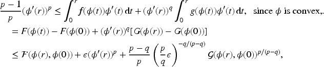
Using this, condition (H-2) and the Dominated Convergence Theorem (due to conditions (H-4), (H-5)), and the assumption that

u_{j} (0) \to \infty

, we note that the right-hand side converges to zero, which is an obvious contradiction. Therefore, the sequence

{u_{j} (0)}

must be bounded, as claimed. Recalling that each

u_{j}

is convex, there is⁴ a sequence

{r_{j}}

of points in

(0, R)

such that

u_{j}^{'} (r) \leq 1

[0, r_{j}]

and

u_{j}^{'} (r_{j}) = 1

for all

j

. Thus,

u_{j} (r_{j}) - u_{j} (0) = \int_{0}^{r_{j}} u_{j}^{'} (t) d t, 0 \leq r_{j} \leq R .

Therefore

{u_{j} (r_{j})}

is bounded. Proceeding as in the steps leading up to (6.4), we find that

\begin{aligned} \frac{1}{n (p - 1)} (β_{j} - u_{j} (r_{j})) & = \frac{1}{n (p - 1)} (u_{j} (R) - u_{j} (r_{j})) \leq \int_{u_{j}^{'} (r_{j})}^{\infty} \frac{s^{p - 1}}{H (u_{j} (r_{j}), s)} d s \\ = \int_{1}^{\infty} \frac{s^{p - 1}}{H (u_{j} (r_{j}), s)} d s \leq \int_{1}^{\infty} \frac{s^{p - 1}}{H (0, s)} d s < \infty . \end{aligned}

This is a contradiction.

Theorem 6.2

Suppose $H \in C (R \times R_{0}^{+}, R_{0}^{+})$ satisfies (H-2) $\sim$ (H-5), and (H-c). If $Ω \subseteq R^{n}$ is a bounded $C^{1}$ open set with the interior ball condition, then Problem ( $H$ ) has no non-negative solution in $W_{l o c}^{1, p} (Ω) \cap C (Ω)$ .

Proof.

For the sake of contradiction, let us suppose that Problem ( $H$ ) admits a non-negative solution $u \in W_{l o c}^{1, p} (Ω) \cap C (Ω)$ . Since $Ω$ satisfies the interior ball condition, we pick $B_{R} := B (x_{0}, R) \subseteq Ω$ such that ${\bar{B}}_{R} \cap \bar{Ω} = {y_{0}}$ . Let $x_{ϵ} := x_{0} - ϵ ν (y_{0})$ , where $ν (y_{0})$ is the outward unit normal to $\partial Ω$ at $y_{0}$ . Observe that $B (x_{ϵ}, R) ⋐ Ω$ for $ϵ$ sufficiently small. Let $B_{ϵ} := B (x_{ϵ}, R)$ and $β_{ϵ} := max_{\partial B_{ϵ}} u$ . Note that $β_{ϵ} \to \infty$ as $ϵ \to 0$ . Moreover, we have

{\begin{aligned} Δ_{p} u & = H (u, | D u |) & in B (x_{ϵ}, R) \\ u & \leq β_{ϵ} & on \partial B (x_{ϵ}, R) . \end{aligned}

Fix

M > ess sup_{{\bar{B}}_{ϵ}} | D u |^{2}

, and let us consider the Dirichlet problem⁵

{\begin{aligned} Δ_{p} w & = H (w, χ (| D w |^{2})) & in B (x_{ϵ}, R) \\ w & = β_{ϵ} & on \partial B (x_{ϵ}, R), \end{aligned}

(6.6)

where

χ (t) = \sqrt{t}

for

0 \leq t \leq M

and

χ (t) = \sqrt{M}

for

t \geq M

. On noting that

w_{1} \equiv 0

is a subsolution, and

w_{2} \equiv β_{ϵ}

is a supersolution, we can find a solution

w_{ϵ} \in W^{1, p} (B_{ϵ})

of Problem (6.6) such that

0 \leq w_{ϵ} \leq β_{ϵ}

B_{ϵ}

, see Véron (2017, Corollary 1.4.5). Thus, we see that

w_{ϵ} \in C^{1, α} ({\bar{B}}_{ϵ})

for some

0 < α < 1

. This follows from Lieberman (1988, Theorem 1).

Observe that $Δ_{p} u = H (u, χ (| D u |^{2}))$ . By the standard comparison principle for the homogeneous $p$ -Laplace equation we see that $0 \leq u \leq β_{ϵ}$ in $B_{ϵ}$ . Therefore, we conclude that $u \in C^{1, α} ({\bar{B}}_{ϵ})$ for some constant $0 < α < 1$ (see Lieberman 1988, Theorem 1). Since $χ (t) \leq \sqrt{t}$ for $t \geq 0$ , we use condition (H-3) to note that $w_{ϵ}$ is a supersolution of $Δ_{p} w = H (w, | D w |)$ in $B (x_{ϵ}, R)$ . Moreover, $u \leq w_{ϵ}$ on the boundary $\partial B (x_{ϵ}, R)$ . From this, and the comparison principle, that is, assumption (H-c), we find $u \leq w_{ϵ}$ in $B_{ϵ}$ . Note that $β_{ϵ} = u (z) = w_{ϵ} (z)$ for some $z \in \partial B_{ϵ}$ . Therefore

\frac{\partial w_{ϵ}}{\partial ν} (z) \leq \frac{\partial u}{\partial ν} (z),

where

ν

is the outer unit normal at

z

. We observe that

w_{ϵ}

is radial and convex. Therefore, setting

w_{ϵ} (x) = v_{ϵ} (r),

where

r := | x - x_{ϵ} |)

we see that

v_{ϵ}^{'} (r) \leq v_{ϵ}^{'} (R) \leq | D u (z) | < \sqrt{M} .

In other words $| D w_{ϵ} |^{2} < M$ in $B_{ϵ}$ , and consequently $w_{ϵ}$ is a solution of (6.5) in $B_{ϵ}$ , with $β := β_{ϵ}$ . On taking $ϵ$ sufficiently small, we see that (6.5) has a non-negative solution in the ball $B_{ϵ} = B (x_{ϵ}, R)$ of radius $R$ , for arbitrarily large $β_{ϵ}$ . But this contradicts Lemma 6.1, and as a consequence we conclude that Problem ( $H$ ) cannot have a solution in $W_{l o c}^{1, p} (Ω) \cap C (Ω)$ .

Proof of Theorem 3.4. The theorem follows from Theorem 6.2 once it is shown that $H (s, t) := f (s) + g (s) t^{q}$ satisfies all the conditions (H-2) $\sim$ (H-5), and (H-c). Obviously, (H-c) holds by Theorem A. Since $q > p$ , it is also obvious that (H-4) holds. One can also verify that (H-2), (H-3), and (H-5) hold. This finishes the proof of Theorem 3.4.

7. Asymptotic Boundary Estimates and Uniqueness

In this section, we suppose that $0 < q \leq p$ , and assume that $f, g : R \to R$ are continuous and non-decreasing functions.

Let us also record the following simple but useful fact. Suppose that $v \in C^{1} (Ω),$ with $Δ_{p} v \in L_{l o c}^{1} (Ω)$ , and $ϕ$ is a $C^{2}$ function on an open interval $J$ that contains the image $v (Ω) := {v (x) : x \in Ω}$ , and that $ϕ^{'} \neq 0$ in $J$ . Direct computation shows that $w := ϕ (v)$ belongs to $C^{1} (Ω)$ , and satisfies

Δ_{p} w = (p - 1) | ϕ^{'} (v) |^{p - 2} ϕ^{″} (v) | D v |^{p} + | ϕ^{'} (v) |^{p - 2} ϕ^{'} (v) Δ_{p} v in Ω .

(7.1)

Let $Ω$ be a bounded $C^{2}$ domain, and let $d_{Ω} (x)$ denote the distance of $x \in Ω$ to the boundary $\partial Ω$ . Then, there is $μ > 0$ such that $d_{Ω} \in C^{2} ({\bar{Ω}}_{μ})$ , where

Ω_{μ} := {x \in Ω : 0 < d_{Ω} (x) < μ} .

Note that we have

| D d_{Ω} | = 1

Ω_{μ}

. See Gilbarg and Trudinger (1983, Chapter 14) for a discussion on these assertions.

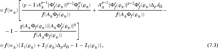
Proof of Theorem 3.5. Let us first consider (3.1). Since $f \in {R V}_{σ}$ with $σ > p - 1$ , we see that $f$ satisfies (i) of (2.1). Therefore, $Φ_{f}$ as given in (I) of (2.2), is well-defined. With $0 < ε < 1$ we set

A_{\pm, ε} = {(\frac{p - 1}{p (1 \pm ε)})}^{\frac{1}{σ + 1 - p}} .

For brevity, we will write $A_{\pm}$ for $A_{\pm, ε}$ . Let $0 < ρ < μ$ , and let us consider the functions $w_{\pm} := A_{\pm} Φ_{f} (d_{Ω} \pm ρ)$ in $O_{ρ}^{\pm},$ where

O_{ρ}^{-} := {x \in Ω : ρ < d_{Ω} < μ}, and O_{ρ}^{+} := {x \in Ω : 0 < d_{Ω} < μ - ρ} .

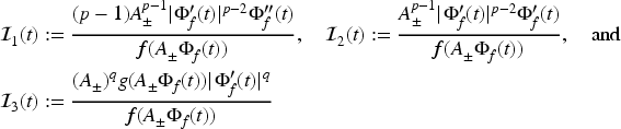
For convenience we will write

ϱ_{\pm}

for

d_{Ω} \pm ρ

. Using (7.1) we compute

\begin{aligned} Δ_{p} w_{\pm} - f (w_{\pm}) - g (w_{\pm}) | D w_{\pm} |^{q} & = [(p - 1) A_{\pm}^{p - 1} | Φ_{f}^{'} (ϱ_{\pm}) |^{p - 2} Φ_{f}^{″} (ϱ_{\pm}) | D d_{Ω} |^{p} \\ + A_{\pm}^{p - 1} | Φ_{f}^{'} (ϱ_{\pm}) |^{p - 2} Φ_{f}^{'} (ϱ_{\pm}) Δ_{p} d_{Ω}] - f (w_{\pm}) - g (w_{\pm}) | D w_{\pm} |^{q} \end{aligned}

(7.2)

\begin{aligned} = f (w_{\pm}) [\frac{(p - 1) A_{\pm}^{p - 1} | Φ_{f}^{'} (ϱ_{\pm}) |^{p - 2} Φ_{f}^{″} (ϱ_{\pm})}{f (A_{\pm} Φ_{f} (ϱ_{\pm}))} + \frac{A_{\pm}^{p - 1} | Φ_{f}^{'} (ϱ_{\pm}) |^{p - 2} Φ_{f}^{'} (ϱ_{\pm}) Δ_{p} d_{Ω}}{f (A_{\pm} Φ_{f} (ϱ_{\pm}))} - \\ - 1 - \frac{g (A_{\pm} Φ_{f} (ϱ_{\pm})) | A_{\pm} Φ_{f}^{'} (ϱ_{\pm}) |^{q}}{f (A_{\pm} Φ_{f} (ϱ_{\pm}))}] \\ = f (w_{\pm}) {I_{1} (ϱ_{\pm}) + I_{2} (ϱ_{\pm}) Δ_{p} d_{Ω} - 1 - I_{3} (ϱ_{\pm})}, \end{aligned}

(7.3)

where

\begin{aligned} I_{1} (t) & := \frac{(p - 1) A_{\pm}^{p - 1} | Φ_{f}^{'} (t) |^{p - 2} Φ_{f}^{″} (t)}{f (A_{\pm} Φ_{f} (t))}, I_{2} (t) := \frac{A_{\pm}^{p - 1} | Φ_{f}^{'} (t) |^{p - 2} Φ_{f}^{'} (t)}{f (A_{\pm} Φ_{f} (t))}, and \\ I_{3} (t) & := \frac{(A_{\pm})^{q} g (A_{\pm} Φ_{f} (t)) | Φ_{f}^{'} (t) |^{q}}{f (A_{\pm} Φ_{f} (t))} \end{aligned}

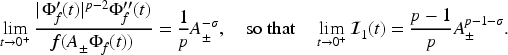
Let us first make note of the following (see Appendix B).

\frac{| Φ_{f}^{'} (t) |^{p - 2} Φ_{f}^{″} (t)}{f (Φ_{f} (t))} = \frac{1}{p}, lim_{t \to 0^{+}} \frac{| Φ_{f}^{'} (t) |^{p - 2} Φ_{f}^{'} (t)}{f (Φ_{f} (t))} = 0, and lim_{t \to 0^{+}} \frac{t Φ_{f}^{'} (t)}{Φ_{f} (t)} = - \frac{p}{σ + 1 - p} .

Again, using the fact that

f \in {R V}_{σ}

we get

\begin{aligned} lim_{t \to 0^{+}} \frac{| Φ_{f}^{'} (t) |^{p - 2} Φ_{f}^{″} (t)}{f (A_{\pm} Φ_{f} (t))} = \frac{1}{p} A_{\pm}^{- σ}, so that lim_{t \to 0^{+}} I_{1} (t) = \frac{p - 1}{p} A_{\pm}^{p - 1 - σ} . \end{aligned}

Also, since

Δ_{p} d_{Ω}

is bounded on

{\bar{Ω}}_{μ}

, we have

lim_{t \to 0^{+}} I_{2} (t) Δ_{p} d_{Ω} = 0

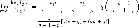
Furthermore, we write

\begin{aligned} \frac{\log (A_{\pm}^{- q} I_{3} (t))}{\log t} \\ = \frac{\log g (A_{\pm} Φ_{f} (t))}{\log A_{\pm} Φ_{f} (t)} \cdot \frac{\log A_{\pm} Φ_{f} (t)}{\log t} - \frac{\log f (A_{\pm} Φ_{f} (t))}{\log A_{\pm} Φ_{f} (t)} \cdot \frac{\log A_{\pm} Φ_{f} (t)}{\log t} + q \frac{\log | Φ_{f}^{'} (t) |}{\log t} . \end{aligned}

(7.4)

Recalling that $f \in {RV}_{σ}$ for $σ > p - 1$ , and $g \in {RV}_{κ}$ for $κ > p - 1 - q$ we find from (7.4), see Appendix B, the following:

\begin{aligned} lim_{t \to 0^{+}} \frac{\log I_{3} (t)}{\log t} & = - \frac{κ p}{σ + 1 - p} + \frac{σ p}{σ + 1 - p} + q (- \frac{σ + 1}{σ + 1 - p}) \\ = \frac{1}{σ + 1 - p} [σ (p - q) - (p κ + q)] . \end{aligned}

Since we assume that

\frac{σ - κ}{σ + 1} > \frac{q}{p},

then we find that

lim_{t \to 0^{+}} I_{3} (t) = 0.

Recalling our choice of $A_{\pm} = A_{\pm, ε}$ , we see that

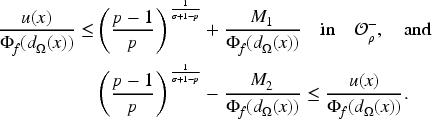
\begin{aligned} lim_{ϱ_{\pm} \to 0} {I_{1} (ϱ_{\pm}) + I_{2} (ϱ_{\pm}) Δ_{p} d_{Ω} - 1 - I_{3} (ϱ_{\pm})} & = (\frac{p - 1}{p}) A_{\pm}^{p - 1 - σ} - 1 \\ = \pm ε . \end{aligned}

(7.5)

As a consequence of (7.5), we observe from equation (7.3) that, for sufficiently small

μ

, we have the following inequalities.

Δ_{p} w_{+} \geq f (w_{+}) + g (w_{+}) | D w_{+} |^{q} in O_{ρ}^{+}, and Δ_{p} w_{-} \leq f (w_{-}) + g (w_{-}) | D w_{-} |^{q} in O_{ρ}^{-} .

Let

M_{1} := sup {u (x) : d_{Ω} (x) \geq μ}

and

M_{2} := A_{+} Φ_{f} (μ)

. Then

u \leq w_{-} + M_{1} on \partial O_{ρ}^{-}, and w_{+} \leq u + M_{2} on \partial O_{ρ}^{+} .

Since

f

and

g

are non-decreasing we see that

w_{-} + M_{1}

and

u + M_{2}

are supersolutions of (5.1) in

O_{ρ}^{-}

and

Ω

, respectively. Note that

w_{-} + M_{1} \in W_{l o c}^{1, \infty} (O_{ρ}^{-})

and

w_{+} \in W_{l o c}^{1, \infty} (O_{ρ}^{+})

. Therefore, by the comparison principle, Theorem A we conclude that

u \leq w_{-} + M_{1} in O_{ρ}^{-} and w_{+} \leq u + M_{2} in O_{ρ}^{+} .

In other words we have

\frac{u}{Φ_{f} (d_{Ω} - ρ)} \leq A_{-, ε} + \frac{M_{1}}{Φ_{f} (d_{Ω} - ρ)} in O_{ρ}^{-} and A_{+, ε} - \frac{M_{2}}{Φ_{f} (d_{Ω} + ρ)} \leq \frac{u}{Φ_{f} (d_{Ω} + ρ)} in O_{ρ}^{+} .

Letting

ρ \to 0^{+}

followed by taking the limit as

ε \to 0^{+}

we find the following in

O_{ρ}^{+}

\begin{aligned} \frac{u (x)}{Φ_{f} (d_{Ω} (x))} \leq & {(\frac{p - 1}{p})}^{\frac{1}{σ + 1 - p}} + \frac{M_{1}}{Φ_{f} (d_{Ω} (x))} in O_{ρ}^{-}, and \\ {(\frac{p - 1}{p})}^{\frac{1}{σ + 1 - p}} - \frac{M_{2}}{Φ_{f} (d_{Ω} (x))} \leq \frac{u (x)}{Φ_{f} (d_{Ω} (x))} . \end{aligned}

Finally, taking the limit as $d_{Ω} (x) \to 0^{+}$ we get the desired conclusion in (3.1).

Next, we take up (3.2). The method is essentially the same as the (3.1) case, and thus we will be brief. Since $g \in {R V}_{κ}$ for $κ > p - 1 - q$ we should note that $g$ satisfies (ii) of (2.1). Therefore, the function $Φ_{g}$ in (II) of (2.2) is well-defined. For $0 < ε < 1$ , let

A_{\pm} := A_{\pm, ε} = {(\frac{p - 1}{(p - q) (1 \pm ε)})}^{\frac{1}{κ - (p - 1 - q)}}, and w_{\pm} := A_{\pm} Φ_{g} (d_{Ω} \pm ρ) in O_{ρ}^{\pm} .

Starting with (7.2), we have

\begin{aligned} Δ_{p} w_{\pm} - f (w_{\pm}) - g (w_{\pm}) | D w_{\pm} |^{q} = g (w_{\pm}) | D w_{\pm} |^{q} [\frac{(p - 1) A_{\pm}^{p - 1 - q} | Φ_{g}^{'} (ϱ_{\pm}) |^{p - q - 2} Φ_{g}^{″} (ϱ_{\pm})}{g (A_{\pm} Φ_{g} (ϱ_{\pm}))} + \\ + \frac{A_{\pm}^{p - 1 - q} | Φ_{g}^{'} (ϱ_{\pm}) |^{p - q - 2} Φ_{g}^{'} (ϱ_{\pm}) Δ_{p} d_{Ω}}{g (A_{\pm} Φ_{g} (ϱ_{\pm}))} - \frac{A_{\pm}^{- q} | Φ_{g}^{'} (ϱ_{\pm}) |^{- q} f (A_{\pm} Φ_{g} (ϱ_{\pm}))}{g (A_{\pm} Φ_{g} (ϱ_{\pm}))} - 1] \\ = g (w_{\pm}) | D w_{\pm} |^{q} {J_{1} (ϱ_{\pm}) + J_{2} (ϱ_{\pm}) Δ_{p} d_{Ω} - J_{3} (ϱ_{\pm}) - 1}, \end{aligned}

where

\begin{aligned} J_{1} (t) & := \frac{(p - 1) A_{\pm}^{p - 1 - q} | Φ_{g}^{'} (t) |^{p - q - 2} Φ_{g}^{″} (t)}{g (A_{\pm} Φ_{g} (t))}, J_{2} (t) := \frac{A_{\pm}^{p - 1 - q} | Φ_{g}^{'} (t) |^{p - q - 2} Φ_{g}^{'} (t)}{g (A_{\pm} Φ_{g} (t))}, and \\ J_{3} (t) & := \frac{A_{\pm}^{- q} | Φ_{g}^{'} (t) |^{- q} f (A_{\pm} Φ_{g} (t))}{g (A_{\pm} Φ_{g} (t))} . \end{aligned}

As before (see Appendix B)

lim_{t \to 0^{+}} J_{1} (t) = \frac{p - 1}{p - q} A_{\pm}^{p - q - 1 - κ}, lim_{t \to 0^{+}} J_{2} (t) Δ_{p} d_{Ω} = 0.

Using the assumptions that

f \in R V_{σ}

for

σ > p - 1

and

g \in R V_{κ}

for

κ > p - 1 - q

, we obtain the limit

lim_{t \to 0^{+}} \frac{\log J_{3} (t)}{\log t} = - (- q + σ - κ) \frac{p - q}{κ + 1 - (p - q)} + q = \frac{σ (q - p) + p κ + q}{κ - (p - q - 1)} .

Recall that

κ - (p - 1 - q) > 0

. In this case if we require

\frac{σ - κ}{σ + 1} < \frac{q}{p},

then

lim_{t \to 0^{+}} J_{3} (t) = 0.

The rest of the proof proceeds as in case (3.1).

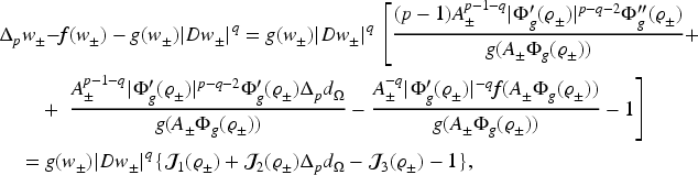
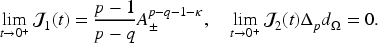
Proof of Theorem 3.6. Let $0 < ρ < μ$ , and $O_{ρ}^{\pm}$ be as in the proof of Theorem 3.5. Recalling that condition (KO) $_{q = p}^{+}$ holds, we note that $Φ$ , as given in (2.3), is well-defined. Upon differentiating the expression (2.3), we find

(- Φ^{'} (t))^{p} = \frac{p}{p - 1} \int_{0}^{Φ (t)} \exp (\frac{p}{p - 1} \int_{s}^{Φ (t)} g (τ) d τ) f (s) d s .

(7.6)

On differentiating both sides of (7.6), we find that

(p - 1) (- Φ^{'} (t))^{p - 2} Φ^{″} (t) = f (Φ (t)) + g (Φ (t)) (- Φ^{'} (t))^{p} .

We employ the same notations used in the proof of Theorem 3.5 for our functions $w_{\pm}$ and sets $Ω_{μ}, O_{ρ}^{\pm}$ , but with $Φ$ defined by (2.3). In other words, we set

w_{\pm} := A_{\pm, ε} Φ (ϱ_{\pm}) in O_{ρ}^{\pm},

where

ϱ_{\pm} := d_{Ω} \pm ρ .

We now compute as in the proof of Theorem 3.5, to obtain

\begin{aligned} Δ_{p} w_{\pm} - f (w_{\pm}) - g (w_{\pm}) | D w_{\pm} |^{p} \\ = [f (w_{\pm}) + g (w_{\pm}) | D w_{\pm} |^{p}] [\frac{(p - 1) A_{\pm}^{p - 1} | Φ^{'} (ϱ_{\pm}) |^{p - 2} Φ^{″} (ϱ_{\pm})}{f (A_{\pm} Φ (ϱ_{\pm})) + g (A_{\pm} Φ (ϱ_{\pm})) | A_{\pm} Φ^{'} (ϱ_{\pm}) |^{p}} + \\ + \frac{A_{\pm}^{p - 1} | Φ^{'} (ϱ_{\pm}) |^{p - 2} Φ^{'} (ϱ_{\pm}) Δ_{p} d_{Ω}}{f (A_{\pm} Φ (ϱ_{\pm})) + g (A_{\pm} Φ (ϱ_{\pm})) | A_{\pm} Φ^{'} (ϱ_{\pm}) |^{p}} - 1] \\ = [f (w_{\pm}) + g (w_{\pm}) | D w_{\pm} |^{p}] [A_{\pm}^{p - 1} \frac{f (Φ (ϱ_{\pm})) + g (Φ (ϱ_{\pm})) | Φ^{'} (ϱ_{\pm}) |^{p}}{f (A_{\pm} Φ (ϱ_{\pm})) + g (A_{\pm} Φ (ϱ_{\pm})) | A_{\pm} Φ^{'} (ϱ_{\pm}) |^{p}} - \\ - \frac{A_{\pm}^{p - 1} | Φ^{'} (ϱ_{\pm}) |^{p - 1} Δ_{p} d_{Ω}}{f (A_{\pm} Φ (ϱ_{\pm})) + g (A_{\pm} Φ (ϱ_{\pm})) | A_{\pm} Φ^{'} (ϱ_{\pm}) |^{p}} - 1] \\ = [f (w_{\pm}) + g (w_{\pm}) | D w_{\pm} |^{p}] {I_{1} (ϱ_{\pm}) - 1 - I_{2} (ϱ_{\pm}) Δ_{p} d_{Ω}}, \end{aligned}

where

\begin{aligned} I_{1} (t) & := A_{\pm}^{p - 1} \frac{f (Φ (t)) + g (Φ (t)) | Φ^{'} (t) |^{p}}{f (A_{\pm} Φ (t)) + g (A_{\pm} Φ (t)) | A_{\pm} Φ^{'} (t) |^{p}}, and \\ I_{2} (t) & := \frac{A_{\pm}^{p - 1} | Φ^{'} (t) |^{p - 1}}{f (A_{\pm} Φ (t)) + g (A_{\pm} Φ (t)) | A_{\pm} Φ^{'} (t) |^{p}} . \end{aligned}

Note that, from (7.6), we have

\begin{aligned} | Φ^{'} (t) |^{p} & = \frac{p}{p - 1} \int_{0}^{Φ (t)} \exp (\frac{p}{p - 1} \int_{s}^{Φ (t)} g (τ) d τ) f (s) d s \end{aligned}

(7.7)

\begin{aligned} \geq \int_{0}^{Φ (t)} f (s) d s = F (Φ (t)) . \end{aligned}

(7.8)

Therefore,

\frac{f (Φ (t))}{g (A_{\pm} Φ (t)) | Φ^{'} (t) |^{p}} \leq \frac{f (Φ (t))}{g (A_{\pm} Φ (t)) F (Φ (t))} \leq \frac{2}{Φ (t) g (A_{\pm} Φ (t))} \frac{f (Φ (t))}{f (Φ (t) / 2)} .

Similar inequality holds with the numerator replaced by

f (A_{\pm} Φ (t))

. Therefore, recalling that

f \in R V_{σ}, g \in R V_{κ}

and that

Φ (t) \to \infty

t \to 0^{+}

, we see that,

lim_{t \to 0^{+}} I_{1} (t) = A_{\pm}^{- 1} lim_{t \to 0^{+}} \frac{g (Φ (t))}{g (A_{\pm} Φ (t))} = A_{\pm}^{- κ - 1} .

(7.9)

From (7.6), and (7.8), we see that

I_{2} \leq \frac{1}{A_{\pm}} \frac{1}{g (A_{\pm} Φ (t)) | Φ^{'} (t) |} \leq \frac{1}{A_{\pm}} \frac{1}{g (A_{\pm} Φ (t)) F (Φ (t))^{\frac{1}{p}}} .

(7.10)

Clearly, since $f (τ) > 0$ for some $τ > 0$ , it follows from (7.10) that⁶

lim_{t \to 0^{+}} I_{2} (t) = 0.

(7.11)

For

0 < ε < 1

, let us take the constants

A_{\pm, ε} := {(\frac{1}{1 \pm ε})}^{\frac{1}{κ + 1}},

where

κ

is the index of

g

Since $Δ_{p} d_{Ω}$ is bounded in $Ω_{μ}$ , it follows from (7.9) and (7.11) that

lim_{ϱ_{\pm} \to 0} {I_{1} (ϱ_{\pm}) - 1 - I_{2} (ϱ_{\pm}) Δ_{p} d_{Ω}} = A_{\pm}^{- κ - 1} - 1 = \pm ϵ .

(7.12)

From (7.12), for sufficiently small

μ > 0

, we have

Δ_{p} w_{+} \geq f (w_{+}) + g (w_{+}) | D w_{+} |^{q} i n O_{ρ}^{+} a n d Δ_{p} w_{-} \leq f (w_{-}) + g (w_{-}) | D w_{-} |^{q} i n O_{ρ}^{-} .

The rest of the argument proceeds as in the proof of Theorem 3.5.

Finally, we turn to uniqueness of solutions to Problem $(A^{+})$ . We need the following simple lemma on comparison principle.

Lemma 7.1

Let $p > 1$ , and $0 < q \leq p$ . Suppose that $f, g : R \to R$ satisfy condition (A-1) $^{+}$ . Let $u, v \in W_{l o c}^{1, \infty} (Ω)$ such that

Δ_{p} u \geq f (u) + g (u) | D u |^{q} and Δ_{p} v \leq f (v) + g (v) | D v |^{q} in Ω .

lim_{d_{Ω} (x) \to 0^{+}} \frac{u (x)}{v (x)} < 1,

then

u \leq v

Ω

Proof.

Suppose to the contrary, $u > v$ at some point in $Ω$ . Consider the open set $O := {u > v}$ . By assumption we have $O ⋐ Ω$ and $u = v$ on $\partial O$ . Therefore, by the comparison principle, Theorem A, we have $u \leq v$ in $O$ , which is a clear contradiction.

We are now ready to prove our uniqueness result for solutions to $(A^{+})$ .

Proof of Theorem 3.7. Let $u, v \in W_{l o c}^{1, \infty} (Ω)$ be two non-negative solutions of $(A^{+})$ . Then it follows from Theorem 3.5, and Theorem 3.6 that

lim_{d_{Ω} (x) \to 0^{+}} \frac{u (x)}{v (x)} = 1.

Let

w_{ϵ} = (1 + ϵ) v

for

ε > 0

. Then clearly

lim_{d_{Ω} (x) \to 0^{+}} \frac{u (x)}{w_{ϵ} (x)} < 1.

Moreover, using assumption (N-D), we obtain

\begin{aligned} Δ_{p} w_{ϵ} & = (1 + ϵ)^{p - 1} Δ_{p} v \\ = (1 + ϵ)^{p - 1} f (v) + (1 + ϵ)^{p - 1 - q} g (v) | D (1 + ϵ) v |^{q} \\ \leq f (w_{ϵ}) + g (w_{ϵ}) | D w_{ϵ} |^{q} . \end{aligned}

Therefore, by Lemma 7.1 we conclude that

u \leq w_{ϵ}

Ω

. Since

ϵ

is arbitrary we find that

u \leq v

Ω

. A similar argument shows that

v \leq u

Ω

, thereby proving uniqueness.

8. A Few Examples

I. Let $Ω \subset R^{n}$ be a bounded open set, and consider the problem

{\begin{array}{rcll} Δ_{p} u & = & | u |^{γ - 1} u + | D u |^{q}, & in Ω \\ u & = & \infty & on \partial Ω . \end{array}

(E-1)

Let

γ > p - 1

. Then Problem (E-1) admits a non-negative solution in

W_{l o c}^{1, \infty} (Ω)

for any

0 < q \leq p

(per (I) of Corollary 5.3). If

Ω

has

C^{2}

boundary,

γ > p - 1, p - 1 < q < p

, and

γ \neq q / (p - q)

, then the solution is unique in

W_{l o c}^{1, \infty} (Ω)

. When

q = p

, then the solution is unique in

W_{l o c}^{1, \infty} (Ω)

for any

γ > 0

(cf. Bandle and Giarrusso 1996 when

p = 2

Now, let $0 < γ \leq p - 1$ . Then Problem (E-1) has a non-negative solution in $W_{l o c}^{1, \infty} (Ω)$ when $p - 1 < q \leq p$ (see (I) of Corollary 5.3), but no non-negative solution in $W_{l o c}^{1, \infty} (Ω)$ if $0 < q \leq p - 1$ , as $(KO)_{q < p}^{+}$ fails in this case.

II. Now we look at the problem

{\begin{array}{rcll} Δ_{p} u & = & f (u) + g (u) | D u |^{p}, & in Ω \\ u & = & \infty & on \partial Ω, \end{array}

(E-2)

where

Ω \subset R^{n}

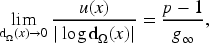
is a bounded open set with

C^{2}

boundary. Suppose

f

and

g

meet the assumptions of Theorem 3.1, and Theorem 3.6, and assume that (N-D) holds as well. If

f (s) \exp (- \frac{p}{p - 1} G (s))

is integrable over

R_{0}^{+}

, then the unique non-negative solution

u

of Problem (E-2) satisfies

lim_{d_{Ω} (x) \to 0} \frac{u (x)}{| \log d_{Ω} (x) |} = \frac{p - 1}{g_{\infty}},

where

g_{\infty} := lim_{t \to \infty} g (t)

. This follows from Theorem 3.6, and the limit (see Appendix C)

lim_{t \to 0 +} \frac{Φ (t)}{| \log t |} = \frac{p - 1}{g_{\infty}} .

(8.1)

Here,

Φ

is the function defined in (2.3).

Footnotes

Acknowledgments

This work was supported by ISP (International Science Program) of Uppsala University, Sweden.

Funding

The authors received no financial support for the research, authorship and/or publication of this article.

Conflicting Interests

The authors declared no potential conflicts of interest with respect to the research, authorship, and/or publication of this article.

Notes

Appendix A. Existence of Solutions to Initial-Value Problems

While the content of this appendix is probably not new, we were unable to find sources that present the results in the form used in the paper. Therefore, we have decided to include a complete and comprehensive discussion.

In the first part of this appendix, we study solutions to the IVP ( ) for any given $a > 0$ . In fact, it is helpful to consider the following more general IVP with given constants $a > 0, b \geq 0$ and $r_{0} \geq 0$ , where we assume $b = 0$ if $r_{0} = 0$ . (${\bf IVP}(r_0;a,b)$)

{\begin{array}{rcll} r^{1 - n} {(r^{n - 1} | ϕ^{'} (r) |^{p - 2} ϕ^{'} (r))}^{'} & = & H (ϕ (r), | ϕ^{'} (r) |), 0 \leq r < R, \\ ϕ (r_{0}) & = & a, ϕ^{'} (r_{0}) = b, \end{array}

under the assumption that

H : R \times R_{0}^{+} \to R

is a continuous function that satisfies (H-1), together with the following condition:

(H-2)

^{*}

$H (a, b) > 0$ .

We prove the following.

Proof. Since $H (a, b) > 0$ , we use the continuity of $H$ to fix $β > 0$ such that $H (s, t) \geq 0$ for all $(s, t) \in [a - β, a + β] \times [(b - β)^{+}, b + β]$ . Here, we are using the standard notation $m^{+} := max {0, m}$ . Let us set

M := max {| H (s, t) | : (s, t) \in [a - β, a + β] \times [(b - β)^{+}, b + β]} .

Also let

J_{α} := [r_{0}, r_{0} + α],

where

α > 0

is to be specified later⁷

We consider the Banach space $B := C^{1} (J_{α})$ , with its standard norm

‖ ϕ ‖_{C^{1}} = ‖ ϕ ‖_{L^{\infty} (J_{α})} + ‖ ϕ^{'} ‖_{L^{\infty} (J_{α})},

as well as the following non-empty, closed and convex subset

A := {ϕ \in B : ϕ (r_{0}) = a, ϕ^{'} (r_{0}) = b, | ϕ (r) - a | \leq β, | ϕ^{'} (r) - b | \leq β \forall r \in J_{α}} .

We define

T : A \to C (J_{α})

T ϕ (r) := a + \int_{r_{0}}^{r} {[t^{1 - n} (r_{0}^{n - 1} b^{p - 1} + \int_{r_{0}}^{t} s^{n - 1} H (ϕ (s), ϕ^{'} (s)) d s)]}^{\frac{1}{p - 1}} d t, r \in J_{α} .

Clearly,

T ϕ

is differentiable in

J_{α},

and for

r_{0} \leq r < r_{0} + α

we have (A.1)

(T ϕ)^{'} (r) = {[r^{1 - n} (r_{0}^{n - 1} b^{p - 1} + \int_{r_{0}}^{r} s^{n - 1} H (ϕ (s), ϕ^{'} (s)) d s)]}^{\frac{1}{p - 1}} .

Given

r_{0} \leq s < t < r_{0} + α

we estimate

| (T ϕ)^{'} (t) - (T ϕ)^{'} (s) |

as follows. First we estimate (A.2)

\begin{aligned} | \int_{r_{0}}^{t} {(\frac{τ}{t})}^{n - 1} H (ϕ (τ), ϕ^{'} (τ)) d τ - \int_{r_{0}}^{s} {(\frac{τ}{s})}^{n - 1} H (ϕ (τ), ϕ^{'} (τ)) d τ | \\ \leq \int_{r_{0}}^{s} [{(\frac{τ}{s})}^{n - 1} - {(\frac{τ}{t})}^{n - 1}] | H (ϕ (τ), ϕ^{'} (τ)) | d τ + \int_{s}^{t} {(\frac{τ}{t})}^{n - 1} H (ϕ (τ), ϕ^{'} (τ)) d τ \\ \leq (\frac{M}{n}) [\frac{s^{n}}{s^{n - 1}} - \frac{s^{n}}{t^{n - 1}} + \frac{t^{n} - s^{n}}{t^{n - 1}}] \leq (\frac{2 t M}{n}) [1 - {(\frac{s}{t})}^{n}] \\ \leq 2 M | t - s |, r_{0} \leq s < t < r_{0} + α . \end{aligned}

Moreover, if

r_{0} > 0

we have (A.3)

| {(\frac{r_{0}}{t})}^{n - 1} b^{p - 1} - {(\frac{r_{0}}{s})}^{n - 1} b^{p - 1} | = | {(\frac{1}{t})}^{n - 1} - {(\frac{1}{s})}^{n - 1} | r_{0}^{n - 1} b^{p - 1} \leq \frac{n}{r_{0}} b^{p - 1} | t - s | .

Therefore, from the estimates (A.2) and (A.3) we find that (A.4)

\begin{aligned} | {(\frac{r_{0}}{t})}^{n - 1} b^{p - 1} + \int_{r_{0}}^{t} {(\frac{τ}{t})}^{n - 1} H (ϕ (τ), ϕ^{'} (τ)) d τ - \\ - [{(\frac{r_{0}}{s})}^{n - 1} b^{p - 1} + \int_{r_{0}}^{s} {(\frac{τ}{s})}^{n - 1} H (ϕ (τ), ϕ^{'} (τ)) d τ] | \\ \leq {\begin{array}{cl} 2 M | t - s |, & if r_{0} = 0 \\ (\frac{n}{r_{0}} b^{p - 1} + 2 M) | t - s |, & if r_{0} > 0. \end{array} \end{aligned}

We now distinguish between the cases $1 < p < 2$ and $p \geq 2$ . Let us start with the case $p \geq 2$ . We use the inequality $| x^{\frac{1}{p - 1}} - y^{\frac{1}{p - 1}} | \leq | x - y |^{\frac{1}{p - 1}}$ for $x, y > 0$ and the estimate (A.4) to get the following for $r_{0} < s < t < r_{0} + α$ . (A.5)

\begin{aligned} | (T ϕ)^{'} (t) - (T ϕ)^{'} (s) | \\ = | {[{(\frac{r_{0}}{t})}^{n - 1} b^{p - 1} + \int_{r_{0}}^{t} {(\frac{τ}{t})}^{n - 1} H (ϕ (τ), ϕ^{'} (τ)) d τ]}^{\frac{1}{p - 1}} \\ - {[{(\frac{r_{0}}{s})}^{n - 1} b^{p - 1} + \int_{r_{0}}^{s} {(\frac{τ}{s})}^{n - 1} H (ϕ (τ), ϕ^{'} (τ)) d τ]}^{\frac{1}{p - 1}} | \\ \leq Θ_{1}^{\frac{1}{p - 1}} | t - s |^{\frac{1}{p - 1}}, \end{aligned}

where

\begin{aligned} Θ_{1} := Θ_{1} (n, r_{0}, b, p, M) := {\begin{array}{cc} 2 M & i f r_{0} = 0, \\ \frac{n}{r_{0}} b^{p - 1} + 2 M & i f r_{0} \neq 0. \end{array} \end{aligned}

Now let us take up the case $1 < p < 2$ . In this case, we apply the mean-value theorem to (A.5) to get

\begin{aligned} | (T ϕ)^{'} (t) - (T ϕ)^{'} (s) | = \frac{1}{p - 1} | ξ |^{(\frac{2 - p}{p - 1})} \\ \times | (\frac{1}{t^{n - 1}} - \frac{1}{s^{n - 1}}) r_{0}^{n - 1} b^{p - 1} + \int_{r_{0}}^{t} {(\frac{τ}{t})}^{n - 1} H (ϕ (τ), ϕ^{'} (τ)) d τ - \int_{r_{0}}^{s} {(\frac{τ}{s})}^{n - 1} H (ϕ (τ), ϕ^{'} (τ)) d τ |, \end{aligned}

where

ξ := ξ (s, t)

is between

\begin{aligned} {(\frac{r_{0}}{t})}^{n - 1} b^{p - 1} & + \int_{r_{0}}^{t} {(\frac{τ}{t})}^{n - 1} H (ϕ (τ), ϕ^{'} (τ)) d τ, and \\ {(\frac{r_{0}}{s})}^{n - 1} b^{p - 1} + \int_{r_{0}}^{s} {(\frac{τ}{s})}^{n - 1} H (ϕ (τ), ϕ^{'} (τ)) d τ . \end{aligned}

Each is bounded by

b^{p - 1} + α M

. Again, using the estimate (A.4), we find (A.6)

\begin{aligned} | (T ϕ)^{'} (t) - (T ϕ)^{'} (s) | \\ \leq \frac{1}{p - 1} {(b^{p - 1} + α M)}^{\frac{2 - p}{p - 1}} | {(\frac{r_{0}}{t})}^{n - 1} b^{p - 1} + \int_{r_{0}}^{t} {(\frac{τ}{t})}^{n - 1} H (ϕ (τ), ϕ^{'} (τ)) d τ \\ - [{(\frac{r_{0}}{s})}^{n - 1} b^{p - 1} + \int_{r_{0}}^{s} {(\frac{τ}{s})}^{n - 1} H (ϕ (τ), ϕ^{'} (τ)) d τ] | \\ \leq Θ_{1} Θ_{2} | t - s |, \end{aligned}

where

Θ_{2} := \frac{1}{p - 1} {(b^{p - 1} + α M)}^{\frac{2 - p}{p - 1}} .

Thus from (A.5) and (A.6) we conclude that the following holds for all

ϕ \in A

: (A.7)

| (T ϕ)^{'} (t) - (T ϕ)^{'} (s) | \leq Θ max {| t - s |^{\frac{1}{p - 1}}, | t - s |}, t, s \in J_{α},

where

Θ := max {Θ_{1}^{\frac{1}{p - 1}}, Θ_{1} Θ_{2}}

. In particular, on taking

s = r_{0}

in (A.7), we note that (A.8)

| (T ϕ)^{'} (r) - b | \leq Θ max {α^{\frac{1}{p - 1}}, α}, r \in J_{α} .

Therefore we see that $T ϕ \in B$ , and from (A.1) we get (A.9)

| T ϕ (r) - a | = | \int_{r_{0}}^{r} (T ϕ)^{'} (t) d t | \leq α {(M α + b^{p - 1})}^{\frac{1}{p - 1}}, r \in J_{α} .

Clearly

T ϕ (r_{0}) = a

and

(T ϕ)^{'} (r_{0}) = b

, where we use L’Hospital’s Rule when

r_{0} = 0

If we select $α > 0$ sufficiently small, it follows from estimates (A.8) and (A.9) that

| T ϕ (r) - a | \leq β, and | (T ϕ)^{'} (r) - b | \leq β, r \in J_{α} .

On recalling that

T ϕ (r_{0}) = a

and

(T ϕ)^{'} (r_{0}) = b

, we conclude that

T (A) \subseteq A

We now proceed to show that $T$ is continuous on $A$ . Let ${ϕ_{j}}$ be a sequence in $A$ that converges to $ϕ \in A$ . Therefore $ϕ_{j} \to ϕ$ and $ϕ_{j}^{'} \to ϕ^{'}$ uniformly on $J_{α}$ . Let us consider the continuous function $σ (t) = t^{\frac{1}{p - 1}}$ . Note that $H$ and $σ$ are uniformly continuous on $[a - β, a + β] \times [(b - β)^{+}, b + β]$ and $[0, γ],$ where $γ := b^{p - 1} + α M$ , respectively. Hence

r^{1 - n} (r_{0}^{n - 1} b^{p - 1} + \int_{r_{0}}^{r} t^{n - 1} H (ϕ_{j} (t), ϕ_{j}^{'} (t)) d t) \to r^{1 - n} (r_{0}^{n - 1} b^{p - 1} + \int_{r_{0}}^{r} t^{n - 1} H (ϕ (t), ϕ^{'} (t)) d t)

uniformly on

J_{α}

, and therefore

\begin{aligned} (T ϕ_{j})^{'} (r) & = σ [r^{1 - n} (r_{0}^{n - 1} b^{p - 1} + \int_{r_{0}}^{r} t^{n - 1} H (ϕ_{j} (t), ϕ_{j}^{'} (t)) d t)] \\ \to σ [r^{1 - n} (r_{0}^{n - 1} b^{p - 1} + \int_{r_{0}}^{r} t^{n - 1} H (ϕ (t), ϕ^{'} (t)) d t)] = (T ϕ)^{'} (r) \end{aligned}

uniformly on

J_{α} .

Consequently,

T ϕ_{j} (r) = \int_{r_{0}}^{r} (T ϕ_{j})^{'} (t) d t \to \int_{r_{0}}^{r} (T ϕ)^{'} (t) d t = T ϕ (r)

uniformly on

J_{α}

. In other words,

{T ϕ_{j}}

converges to

T ϕ

in the Banach space

B

Finally, let us show that

T (A) := {T ϕ : ϕ \in A}

is relatively compact in

A

. Since

A

is a bounded subset of

B

, and

T (A) \subseteq A

, we see that

T (A)

is a bounded set. Since

{(T ϕ)^{'} : ϕ \in A}

is uniformly bounded on

J_{α}

, it is obvious that

T (A)

is equicontinuous on

J_{α}

. That

{(T ϕ)^{'} : ϕ \in A}

is equicontinuous on

J_{α}

follows from (A.7).

Hence, by the Schauder fixed-point theorem, there is $ϕ \in A$ such that $T ϕ = ϕ$ , that is, (A.10)

ϕ (r) := a + \int_{r_{0}}^{r} {[t^{1 - n} (r_{0}^{n - 1} b^{p - 1} + \int_{r_{0}}^{t} s^{n - 1} H (ϕ (s), ϕ^{'} (s)) d s)]}^{\frac{1}{p - 1}} d t, r \in J_{α} .

Thus we have shown that Problem ( $I V P (r_{0}; a, b)$ ) has a solution $ϕ \in C^{1} ([r_{0}, R))$ in some interval $[r_{0}, R)$ , and differentiating (A.10) we have (A.11)

ϕ^{'} (r) = {[r^{1 - n} (r_{0}^{n - 1} b^{p - 1} + \int_{r_{0}}^{r} s^{n - 1} H (ϕ (s), ϕ^{'} (s)) d s)]}^{\frac{1}{p - 1}}, r_{0} < r < ϱ .

Let

[r_{0}, R)

be the maximal interval of existence of

ϕ

. We claim that

ϕ^{'} > 0

(r_{0}, R)

. To see this, let

S := {r \in (r_{0}, R) : ϕ^{'} (s) > 0 \forall s \in (r_{0}, r)}

. Condition (H-2)

^{*}

shows that

S

is non-empty (as can be seen from (A.11)), and that

r_{0} < ϱ \leq R,

where

ϱ := sup S

. We assume that

ϱ < R

, for otherwise there is nothing to show.

Let us set (A.12)

θ (r) := r^{1 - n} (r_{0}^{n - 1} b^{p - 1} + \int_{r_{0}}^{r} s^{n - 1} H (ϕ (s), ϕ^{'} (s)) d s), r_{0} \leq r < ϱ,

so that

θ (r) := (ϕ^{'} (r))^{p - 1} r_{0} \leq r < ϱ .

From (A.12), it can clearly be seen that

θ

is positive and differentiable on

(r_{0}, ϱ)

. Furthermore, note that (A.13)

\begin{aligned} lim_{r \to r_{0}^{+}} \frac{θ (r) - θ (r_{0})}{r - r_{0}} \\ = lim_{r \to r_{0}} {\frac{1}{r - r_{0}} [{(\frac{r_{0}}{r})}^{n - 1} - 1] b^{p - 1} + \frac{1}{r^{n - 1}} \cdot \frac{1}{r - r_{0}} \int_{r_{0}}^{r} s^{n - 1} H (ϕ (s), ϕ^{'} (s)) d s} \\ = {\begin{array}{cl} \frac{1}{n} H (a, 0) & if r_{0} = 0 \\ - \frac{(n - 1)}{r_{0}} b^{p - 1} + H (a, b) & if r_{0} > 0. \end{array} \end{aligned}

Thus we see that in fact, $θ$ is differentiable on $[r_{0}, ϱ)$ , and invoking condition (H-2) $^{*}$ and (A.13) we conclude that $θ^{'} (0) > 0$ . In fact, if we suppose that $H (a, 0) > 0$ , then for a fixed $r_{0} > 0$ we have $θ^{'} (r_{0}) > 0$ for all sufficiently small $b > 0$ .

Next we use the differentiability of $θ$ on $[r_{0}, ϱ)$ to show that $ϕ^{'}$ is differentiable in $(r_{0}, ϱ)$ . Let $r_{0} < ρ < ϱ$ . We take any $r \in (r_{0}, ϱ) ∖ {ρ}$ . Then, by the Mean–Value theorem applied to $t \mapsto t^{p - 1}$ on the interval $[min {ϕ^{'} (r), ϕ^{'} (ρ)}, max {ϕ^{'} (r), ϕ^{'} (ρ)}]$ , we have

θ (r) - θ (ρ) = (ϕ^{'} (r))^{p - 1} - (ϕ^{'} (ρ))^{p - 1} = (p - 1) (ζ (r))^{p - 2} (ϕ^{'} (r) - ϕ^{'} (ρ))

for some

ζ (r)

between

ϕ^{'} (ρ)

and

ϕ^{'} (r)

. Since

ϕ^{'} > 0

(r_{0}, ϱ)

, we note that

ζ (r) > 0

(r_{0}, ϱ)

. Therefore

\frac{θ (r) - θ (ρ)}{r - ρ} = (p - 1) (ζ (r))^{p - 2} \frac{ϕ^{'} (r) - ϕ^{'} (ρ)}{r - ρ}, r \in (r_{0}, ϱ) ∖ {ρ} .

Note that

ϕ^{'}

is continuous on

(r_{0}, ϱ)

and we recall that

ζ (r)

is between

ϕ^{'} (r)

and

ϕ^{'} (ρ)

. Hence, as

r \to ρ

we see that

ζ (r) \to ζ (ρ) = ϕ^{'} (ρ) \neq 0

. Thus we see that

\frac{ϕ^{'} (r) - ϕ^{'} (ρ)}{r - ρ} = \frac{1}{p - 1} (ζ (r))^{2 - p} \cdot \frac{θ (r) - θ (ρ)}{r - ρ}, r \in (r_{0}, ϱ) ∖ {ρ} .

Taking the limit of both sides we see that (A.14)

\begin{aligned} lim_{r \to ρ} \frac{ϕ^{'} (r) - ϕ^{'} (ρ)}{r - ρ} & = \frac{1}{p - 1} (ϕ^{'} (ρ))^{2 - p} \cdot lim_{r \to ρ} \frac{θ (r) - θ (ρ)}{r - ρ} \\ = \frac{1}{p - 1} (ϕ^{'} (ρ))^{2 - p} θ^{'} (ρ) . \end{aligned}

Hence

ϕ^{″} (ρ)

exists for all

ρ \in (r_{0}, ϱ)

. If

r_{0} > 0

, and

b > 0

, we note that

ϕ^{'}

is also differentiable at

r_{0}

, and therefore in this case we have

ϕ \in C^{2} ([r_{0}, R))

. Moreover, if

p > 2

we see that

ϕ^{'}

is not differentiable at

r_{0} = 0

. On the other, if

1 < p \leq 2

we see that

ϕ^{'}

is differentiable at

r_{0} = 0

. In fact, in this case we have

ϕ^{″} (0) = 0

. Thus, in general, any solution of Problem ( ) in

[r_{0}, ϱ)

belongs to

C^{2} ((r_{0}, ϱ)) \cap C^{1} ([r_{0}, ϱ)) .

Using (A.12) we differentiate $θ$ on $(r_{0}, ϱ)$ to get the following for $r_{0} < r < ϱ$ . (A.15)

θ^{'} (r) = - \frac{n - 1}{r} [r^{1 - n} (r_{0}^{n - 1} b^{p - 1} + \int_{r_{0}}^{r} t^{n - 1} H (ϕ (t), ϕ^{'} (t)) d t)] + H (ϕ (r), ϕ^{'} (r)) .

From (A.12) and (A.15) we also get (A.16)

θ^{'} + \frac{n - 1}{r} θ = H (ϕ (r), ϕ^{'} (r)), r_{0} < r < ϱ .

Observe that

θ^{'}

is continuous on

[r_{0}, ϱ)

As noted before, recall that $θ^{'} (0) > 0$ , and that if $H (a, 0) > 0$ , then $θ^{'} (r_{0}) > 0$ for sufficiently small $b > 0$ . In any case, under the assumption that $θ^{'} (r_{0}) > 0$ we now proceed to show that $θ^{'} \geq 0$ in $[r_{0}, ϱ)$ .

To this end, suppose that $θ^{'} \geq 0$ in $[r_{0}, ϱ)$ is not the case. Then there is $r_{0} < τ_{0} < ϱ$ such that $θ^{'} (τ_{0}) < 0$ . Since $θ$ is continuous on $[r_{0}, τ_{0}]$ it attains its maximum on $[r_{0}, τ_{0}]$ at some $σ \in [r_{0}, τ_{0}]$ . Since $θ^{'} (τ_{0}) < 0 < θ^{'} (r_{0})$ we see that $σ \notin {r_{0}, τ_{0}}$ . That is, $σ \in (r_{0}, τ_{0})$ . Consequently, we can find $τ$ with $r_{0} < σ < τ < τ_{0}$ , close enough to $σ$ such that $θ (τ) > θ (r_{0})$ , and $θ^{'} (τ) \leq 0$ . Let $S := {r \in (r_{0}, σ) : θ (r) = θ (τ)}$ . Since $θ$ is continuous, and $θ (r_{0}) < θ (τ) \leq θ (σ)$ we see that $S$ is non-empty. Let $μ := inf S$ . Since $S$ is a closed set we see that $μ \in S$ . Furthermore, $θ^{'} (μ) \geq 0$ . If this is not the case, and $θ^{'} (μ) < 0$ , then there is $ν \in (r_{0}, μ)$ such that $θ (ν) > θ (μ) = θ (τ)$ . Since $θ (r_{0}) < θ (μ) < θ (ν)$ , we can find $μ^{*} \in (r_{0}, ν)$ such that $θ (μ^{*}) = θ (μ) = θ (τ)$ . But, this contradicts the minimality of $μ$ .

Using (A.16) we find

\begin{aligned} 0 & \leq θ^{'} (μ) - θ^{'} (τ) \\ = - (\frac{n - 1}{μ}) θ (μ) + H (ϕ (μ), ϕ^{'} (μ)) - [- (\frac{n - 1}{τ}) θ (τ) + H (ϕ (τ), ϕ^{'} (τ))] \\ \leq - (n - 1) θ (μ) [\frac{1}{μ} - \frac{1}{τ}], by (H - 1), since ϕ (μ) \leq ϕ (τ), \\ < 0, since θ (μ) > 0 and μ < τ . \end{aligned}

This obvious contradiction shows that

θ^{'} \geq 0

(r_{0}, ϱ)

. As a consequence of (A.14), and recalling that

ϕ^{'} > 0

(r_{0}, ϱ)

, we conclude that

ϕ^{″} \geq 0

(r_{0}, ϱ)

Finally we remark that $θ > 0$ in $(r_{0}, ϱ)$ and $θ^{'} \geq 0$ in $(r_{0}, ϱ)$ , together with (A.16), imply that $H (ϕ, ϕ^{'}) > 0$ in $(r_{0}, ϱ)$ . In fact, from (A.16) we have (A.17)

H (ϕ (r), ϕ^{'} (r)) \geq \frac{n - 1}{r} ϕ^{'} {(r)}^{p - 1}, r_{0} < r < ϱ .

Finally, we note that (A.17) together with (A.11) shows that

ϕ^{'} (ϱ) > 0

. But the continuity of

ϕ^{'}

(r_{0}, R)

, along with the assumption that

ϱ < R,

leads to the contradiction of the definition of

ϱ

ϱ = sup {r \in (r_{0}, R) : ϕ^{'} (s) > 0, \forall s \in (r_{0}, r)}

. Therefore we must have

ϱ = R

, as claimed so that

ϕ^{'} > 0

[r_{0}, R)

, the maximal interval of existence of

ϕ

Furthermore the inequality (A.17) allows us to prove the following. Let $f, g : R \to R$ be non-decreasing continuous functions such that $f (t) > 0$ for $t > 0$ , $f (0) = 0$ , and $g (t) \geq 0$ for $t \geq 0$ . Suppose $ϕ \in C^{2} ((0, R)) \cap C^{1} ([0, R))$ is a solution to ( ) on a maximal interval $[0, R)$ of existence with $R < \infty$ . Recall that $ϕ > 0, ϕ^{'} > 0$ and $ϕ^{″} \geq 0$ in $(0, R)$ . We claim that $ϕ (r) \to \infty$ as $r \to R$ . If this is not the case, say $ϕ (r) \to α \in R^{+}$ as $r \to R$ , then (4.6) implies that $ϕ^{'} (r) \to β \in R^{+}$ as $r \to R$ . Let $\tilde{ϕ}$ be a solution to the IVP IVP( $R$ ; $α$ , $β$ ) on an interval $[R, \tilde{R})$ . According to (A.17) we note that $H (ϕ (R), ϕ^{'} (R)) > 0$ . By (H-1) and (H-2) $^{*}$ we see that $\tilde{ϕ} \in C^{2} ([R, \tilde{R}))$ and $\tilde{ϕ} (R) = ϕ (R)$ and ${\tilde{ϕ}}^{'} (R) = ϕ^{'} (R)$ . In light of this, and (4.1), we can juxtapose $\tilde{ϕ}$ to $ϕ$ to extend $ϕ$ to a solution of ( ) in the larger interval $[0, \tilde{R})$ . This would contradict the maximality of the interval $[0, R)$ .

Appendix B. On Properties of Regularly Varying Functions

To ensure completeness, in this appendix we will provide proofs of the main properties of regularly varying functions that were used in the paper.

$$_{▸} $$ If $h \in R V_{γ}$ is continuous on $[a, \infty)$ and $γ < - 1$ , then $h \in L^{1} ([a, \infty))$ (see Mohammed 2007 for instance). Now suppose $h \in R V_{γ}$ is non-decreasing and continuous on $[a, \infty)$ . If $H$ is the antiderivative of $h$ that vanishes at zero, and if $γ > ρ - 1$ , then it follows from the definition that $H^{- \frac{1}{ρ}} \in R V_{- (γ + 1) / ρ}$ . Since $- (γ + 1) / ρ < - 1$ we see that

\int_{1}^{\infty} \frac{d s}{H {(s)}^{\frac{1}{ρ}}} < \infty .

$$_{▸} $$ Suppose $h$ is continuous and $h \in {R V}_{σ}$ for some $σ > - 1$ . If $H$ is the antiderivative of $h$ that vanishes at zero, then $lim_{t \to \infty} \frac{H (t)}{t H^{'} (t)} = \frac{1}{σ + 1} .$

Proof. This follows from the computation (B.1)

lim_{t \to \infty} \frac{H (t)}{t h (t)} = \int_{0}^{1} lim_{t \to \infty} \frac{h (t s)}{h (t)} d s = \int_{0}^{1} s^{σ} d s = \frac{1}{σ + 1} .

$$_{▸} $$ Suppose that $h$ is continuous on $[0, \infty)$ and suppose, for some $ν > 1$ ,

\int_{1}^{\infty} \frac{d s}{H {(s)}^{\frac{1}{ν}}} < \infty,

where

H

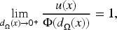
is the antiderivative of

h

that vanishes at zero. Suppose

φ

is defined by

\int_{φ (t)}^{\infty} \frac{d s}{H {(s)}^{\frac{1}{ν}}} = t, t > 0.

Note that

φ (t) \to \infty

t \to 0^{+}

, and that

φ \in C^{2} ((0, ω))

for some

ω > 0

. Moreover, on

(0, ω)

we have (B.2)

\frac{| φ^{'} |^{ν - 2} φ^{'}}{h (φ)} = - \frac{H (φ))^{1 - \frac{1}{ν}}}{h (φ)}, | φ^{'} |^{ν - 2} φ^{″} = \frac{1}{ν} h (φ) .

If we suppose that

h

is non-decreasing, it follows from (B.2) that

lim_{t \to 0^{+}} \frac{| φ^{'} (t) |^{ν - 2} φ^{'} (t)}{h (φ (t))} = 0.

If, furthermore,

h \in {R V}_{σ}

for some

σ > ν - 1

, then (B.3)

\begin{aligned} lim_{t \to 0^{+}} \frac{t φ^{'} (t)}{φ (t)} = \frac{ν}{ν - (σ + 1)} \end{aligned}

(B.4)

\begin{aligned} lim_{t \to 0^{+}} \frac{t φ^{″} (t)}{φ^{'} (t)} = \frac{σ + 1}{ν - (σ + 1)} \end{aligned}

Proof.

Direct computation shows that

\begin{aligned} lim_{t \to 0^{+}} \frac{φ (t)}{t φ^{'} (t)} & = - lim_{t \to 0^{+}} \frac{φ (t)}{t H (φ (t))^{\frac{1}{ν}}} = - lim_{z \to \infty} \frac{z H {(z)}^{- \frac{1}{ν}}}{\int_{z}^{\infty} H (τ)^{\frac{1}{ν}} d τ} \\ = lim_{z \to \infty} \frac{H {(z)}^{- \frac{1}{ν}} - (1 / ν) z H {(z)}^{- \frac{1}{ν - 1}} h (z)}{H {(z)}^{- \frac{1}{ν}}}, byL'Hospitals' Rule \\ = 1 - \frac{1}{ν} lim_{z \to \infty} \frac{z h (z)}{H (z)} = 1 - \frac{1}{ν} (σ + 1) by (B .1) . \end{aligned}

Note that (B.5)

lim_{z \to \infty} \frac{z H {(z)}^{- \frac{1}{ν}}}{\int_{z}^{\infty} H (τ)^{- \frac{1}{ν}} d τ} = \frac{σ + 1 - ν}{ν} .

To prove the limit in (B.4), let us first note from the limits in (B.1) and (B.5) that

lim_{z \to \infty} \frac{ν H {(z)}^{1 - \frac{1}{ν}}}{h (z) \int_{z}^{\infty} H (τ)^{- \frac{1}{ν}} d τ} = lim_{z \to \infty} (\frac{ν z H {(z)}^{- \frac{1}{ν}}}{\int_{z}^{\infty} H (τ)^{- \frac{1}{ν}} d τ} \cdot \frac{H (z)}{z h (z)}) = (σ + 1 - ν) \cdot \frac{1}{σ + 1} .

Since $φ (t) \to \infty$ as $t \to 0^{+}$ and

\frac{φ^{'} (t)}{t φ^{″} (t)} = - \frac{ν H (φ (t))^{(ν - 1) / ν}}{h (φ (t)) \int_{φ (t)}^{\infty} H {(s)}^{- \frac{1}{ν}} d s}

we obtain the desired limit in (B.4).

lim_{t \to 0^{+}} \frac{φ^{'} (t)}{t φ^{″} (t)} = - \frac{σ + 1 - ν}{σ + 1} . ◼

$$_{▸} $$ If $h \in {R V}_{σ}$ , then $lim_{t \to \infty} \frac{\log h (t)}{\log t} = σ .$

Proof. As noted already in (B.1), we have

lim_{s \to \infty} \frac{s h (s)}{H (s)} = σ + 1.

Setting

y (s) = \frac{s h (s)}{H (s)} - (σ + 1), s \in [a, \infty)

we write (B.6)

\frac{y (s)}{s} = \frac{h (s)}{H (s)} - \frac{σ + 1}{s}, s \in [a, \infty) .

Note that

y

is a continuous function such that

y (s) \to 0

s \to \infty

. Therefore by integrating (B.6) on

[a, t]

for

a < t < \infty

and rearranging we see that

H (t) = c_{0} t^{σ + 1} \exp (\int_{a}^{t} \frac{y (s)}{s} d s), t \in [a, \infty) .

Differentiating this leads to

\begin{aligned} h (t) & = c_{0} (σ + 1) t^{σ} \exp (\int_{a}^{t} \frac{y (τ)}{τ} d τ) + c_{0} t^{σ + 1} \frac{y (t)}{t} \exp (\int_{a}^{t} \frac{y (τ)}{τ} d τ) \\ = c_{0} {(σ + 1) + y (t)} t^{σ} \exp (\int_{a}^{t} \frac{y (τ)}{τ} d τ), t \in (a, \infty) . \end{aligned}

As a consequence of this last relation, we find that

lim_{t \to \infty} \frac{\log h (t)}{\log t} = σ . ◼

$$_{▸} $$ Suppose $h \in C^{1} ((a, \infty))$ such that $lim_{t \to \infty} \frac{t h^{'} (t)}{h (t)} = ϱ .$ If $h > 0$ on $(a, \infty)$ , then $h \in R V_{ϱ}$ .

Proof. We proceed as follows. Let

y (t) := \frac{t h^{'} (t)}{h (t)} - ϱ .

Clearly

y

is continuous on

(a, \infty)

and

y (t) \to 0

t \to \infty

. Moreover we see that

h

satisfies the equation

h^{'} (t) - (\frac{y (t)}{t} + \frac{ϱ}{t}) h (t) = 0.

That is

\frac{d}{d t} [(\exp (- \int_{a}^{t} (\frac{y (τ)}{τ} + \frac{ϱ}{τ}) d τ) h (t))] = 0.

Thus we find

h (t) = c_{0} \exp (\int_{a}^{t} (\frac{y (τ)}{τ} + \frac{ϱ}{τ}) d τ) = c_{0} t^{ϱ} \exp (\int_{a}^{t} \frac{y (τ)}{τ} d τ) .

It follows from this that

h \in R V_{ϱ}

Appendix C. The Limit in ( )

Using the assumption that $f (s) \exp (- \frac{p}{p - 1} G (s))$ is integrable on $R_{0}^{+}$ , we compute (C.1)

\begin{aligned} lim_{t \to 0^{+}} \frac{Φ (t)}{| \log t |} = - lim_{t \to 0^{+}} t Φ^{'} (t) \end{aligned}

(C.2)

\begin{aligned} = lim_{t \to 0^{+}} [{(\int_{0}^{Φ (t)} \exp (\frac{p}{p - 1} \int_{s}^{Φ (t)} g (τ) d τ) f (s) d s)}^{\frac{1}{p}} \\ \times \int_{Φ (t)}^{\infty} {(\int_{0}^{τ} \exp (\frac{p}{p - 1} \int_{s}^{τ} g (ω) d ω) f (s) d s)}^{- \frac{1}{p}} d τ] \\ = {(\int_{0}^{\infty} \exp (- \frac{p}{p - 1} G (s)) f (s) d s)}^{\frac{1}{p}} \\ \times lim_{t \to 0^{+}} \frac{\int_{Φ (t)}^{\infty} {(\int_{0}^{τ} \exp (\frac{p}{p - 1} \int_{s}^{τ} g (ω) d ω) f (s) d s)}^{- \frac{1}{p}} d τ}{\exp (- \frac{1}{p - 1} G (Φ (t)))} = (p - 1) lim_{t \to 0^{+}} \frac{1}{g (Φ (t))} . \end{aligned}

In both (C.1), and (C.2), we have used L’Hospital’s Rule.

References

Alarcón

Quaas

(2013). Large viscosity solutions for some fully nonlinear equations. Nonlinear Differential Equations and Applications, 20, 1453–1472.

Bandle

Essén

(1994). On the solutions of quasilinear elliptic problems with boundary blow-up, partial differential equations of elliptic type (Cortona, 1992). Symposium Mathematics, XXXV, Cambridge University Press, Cambridge, 93–111.

Bandle

Giarrusso

(1996). Boundary blowup for semilinear elliptic equations with nonlinear gradient terms. Advances in Differential Equations, 1, 133–150.

Bhattacharya

Mohammed

(2021). Maximum principles for

k

-Hessian equations with lower order terms on unbounded domains. Journal of Geometric Analysis, 31(4), 3820–3862.

Bieberbach

(1916).

Δ u = e^{u}

und die automorphen funktionen. Mathematische Annalen, 77, 173–212.

Chen

Felmer

Quaas

(2015). Large solutions to elliptic equations involving fractional Laplacian. Annales de l’Institut Henri Poincaré C — Analyse Non Linéaire, 32(6), 1199–1228.

Cîrstea

F.-C.

Rădulescu

(2006). Nonlinear problems with boundary blow-up: A Karamata regular variation theory approach. Asymptotic Analysis, 46(3-4), 275–298.

Cîrstea

F.-C.

Rădulescu

(2007). Boundary blow-up in nonlinear elliptic equations of Bieberbach–Rademacher type. Transactions of the American Mathematical Society, 359(7), 3275–3286.

Díaz

Letelier

(1993). Explosive solutions of quasilinear elliptic equations: Existence and uniqueness. Nonlinear Analysis, 20(2), 97–125.

10.

(2003). Boundary blow-up solutions and their applications (pp. 89–97). World Scientific Publishing Co., Inc. ISBN: 981-238-262-3.

11.

(2004). Asymptotic behavior and uniqueness results for boundary blow-up solutions. Differential Integral Equations, 17(7–8), 819–834.

12.

Guo

(2003). Boundary blow-up solutions and their applications in quasilinear elliptic equations. Journal d’Analyse Mathématique, 89, 277–302.

13.

Ghergu

Radulescu

(1997). Large solutions of quasilinear elliptic equations: Existence and qualitative properties. Bollettino dell’Unione Matematica Italiana B (7), 11, 227–252.

14.

Gilbarg

Trudinger

N. S.

(1983). Elliptic partial differential equations of second order (2nd ed.). Springer.

15.

Gladiali

Porru

(1998). Estimates for explosive solutions to

p

-Laplace equations, Progress in Partial Differential Equations, Vol I (Pont-à-Mousson, 1997), (PP. 177–127). Pitman Re. Notes Math. Ser. 383, Longman, Harlow.

16.

Hörmander

(1983). The Analysis of Partial differential operators I. Springer, Berlin, ix+391 pp.

17.

Karls

Mohammed

(2016). Ahmed solutions of

p

-Laplace equations with infinite boundary values: The case of non-autonomous and non-monotone nonlinearities. Proceedings of the Edinburgh Mathematical Society, 59(4), 959–987.

18.

Keller

J. B.

(1957). On solutions of

Δ u = f (u)

. Communications on Pure and Applied Mathematics, 10, 503–510.

19.

Lair

A. V.

Mohammed

(2023). Necessary and sufficient conditions for the existence of large solutions to semilinear elliptic equations with gradient terms. Journal of Differential Equations, 374, 593–631.

20.

Lasry

J. M.

Lions

P. L.

(1989). Nonlinear elliptic equations with singular boundary conditions and stochastic control with state constraints. Mathematische Annalen, 283, 583–630.

21.

Leonori

Porretta

(2016). Large solutions and gradient bounds for quasilinear elliptic equations. Communications in Partial Differential Equations, 41, 952–998.

22.

Leonori

Porretta

Riey

(2017). Comparison principles for p-Laplace equations with lower order terms. Annali di Matematica Pura ed Applicata, 196(3), 877–903.

23.

Lieberman

(1988). Boundary regularity for solutions of degenerate elliptic equations. Nonlinear Analysis, 12, 1203–1219.

24.

Lieberman

(1991). The natural generalization of the natural conditions of Ladyzhenskaya and Ural’tseva for elliptic equations. Communications in Partial Differential Equations, 16, 311–361.

25.

Lieberman

(2011). Asymptotic behavior and uniqueness of blow-up solution of quasilinear elliptic equation. Journal d’Analyse Mathématique, 115, 213–249.

26.

Matero

(1996). Quasilinear elliptic equations with boundary blow-up. Journal d’Analyse Mathématique, 69, 229–247.

27.

Mohammed

(2007). Boundary asymptotic and uniqueness of solutions to the

p

-Laplacian with infinite boundary values. Journal of Mathematical Analysis and Applications, 325(1), 480–489.

28.

Mohammed

(2010). Existence and uniqueness of nonnegative solutions for boundary blow-up problem. Journal of Mathematical Analysis and Applications, 371, 534–545.

29.

Mohammed

Rădulescu

Vitolo

(2020). Blow-up solutions for fully nonlinear equations: Existence, asymptotic estimates and uniqueness. Advances in Nonlinear Analysis, 9(1), 39–64.

30.

Mohammed

Vitolo

(2019). Large solutions of fully nonlinear equations: Existence and uniqueness. NoDEA Nonlinear Differential Equations Application, 26(6), Article number 42.

31.

Mohammed

Vitolo

(2024a). The effects of nonlinear perturbation terms on comparison principles for the

p

-Laplacian. Bulletin of Mathematical Sciences, 14(2), 2450005.

32.

Mohammed

Vitolo

(2024b). Remarks on comparison principles for p-Laplacian with extension to (p, q)-Laplacian. Bulletin of Mathematical Sciences, 14(3), 2450011.

33.

Osserman

(1957). On the inequality

Δ u \geq f (u)

. Pacific Journal of Mathematics, 7, 1641–1647.

34.

Porretta

(2004). Local estimates and large solutions for some elliptic equations with absorption. Advances in Differential Equations, 9(3-4), 329–351.

35.

Rademacher

(1943). Einige besondere probleme partieller Differentialgleichungen. In Die differential und integralgleichungen der mechnik und physik, I (2nd ed., pp. 838–845). Rosenberg.

36.

Véron

(2017). Local and global aspects of quasilinear degenerate equations: Quasilinear singular elliptic problems. World Scientific.

37.

Zhang

(2006). Existence of large solutions for a semilinear elliptic problem via explosive sub-supersolutions. Electronic Journal of Differential Equations, 2006(2), 1–8.

38.

Zhang

(2014). The existence and boundary behavior of large solutions to semilinear elliptic equations with nonlinear gradient terms. Advances in Nonlinear Analysis, 3(3), 165–185.

39.

Zhang

(2017). Boundary behavior of large solutions to

p

-Laplacian elliptic equations. Nonlinear Analysis Real World Applications, 33, 40–57.

40.

Zhang

(2018). Sharp conditions for the existence of boundary blow-up solutions to the Monge–Ampére equation. Calculus of Variations and Partial Differential Equations, 57(2), article number 30.

41.

Zhang

Feng

(2019). The existence and asymptotic behavior of boundary blow-up solutions to the

k

-Hessian equation. Journal of Differential Equations, 267(8), 4626–4672.

42.

Zhang

Kan

(2023). Sufficient and necessary conditions on the existence and estimates of boundary blow-up solutions for singular

p

-Laplacian equations. Acta Mathematica Scientia (Series B) (Engl. Ed.), 43(3), 1175–1194.

Infinite Boundary Value Problems for the p -Laplacian with Nonlinear Gradient Terms

Abstract

1. Introduction

Theorem 3.1 Existence

Theorem 3.2 Non-existence for the case 0 < q ≤ p

Theorem 3.5 Boundary Asymptotic Estimates for the case 0 < q < p

Theorem 3.7 Uniqueness

4. Preliminaries and Auxiliary Results

Theorem A Comparison Principle

Footnotes

Acknowledgments

Funding

Conflicting Interests

Notes

Appendix A. Existence of Solutions to Initial-Value Problems

Appendix B. On Properties of Regularly Varying Functions

Appendix C. The Limit in ( )

References

Theorem 3.2 Non-existence for the case $0 < q \leq p$

Theorem 3.5 Boundary Asymptotic Estimates for the case $0 < q < p$