Solvability of the Nonlinear Plate Equations in Besov Spaces

Abstract

In this article, we study the solvability of the nonlinear plate equation $u_{t t} - Δ u_{t t} + Δ^{2} u - Δ u_{t} = (- Δ)^{θ} | u |^{λ}$ in $R^{n} \times (0, \infty),$ $n \geq 1,$ for a large class of initial data. We prove the existence and uniqueness of local and global mild solutions in the framework of Besov $B_{p, \infty}^{s} (R^{n})$ -spaces. Our approach relies on time decay estimates in $B_{p, q}^{s} (R^{n})$ for the differential operators $\partial_{t}^{k} Λ_{θ} (t)$ and $\partial_{t}^{k} S (t),$ $k = 0, 1, 2,$ being $Λ_{θ} (t) = S (t) (I - Δ)^{- 1 / 2} (- Δ)^{θ},$ and $S (t)$ the solution of the corresponding linear problem. We also prove the asymptotic stability of global solutions in the same setting.

Keywords

plate equations time decay rates local and global solutions asymptotic stability

1. Introduction

The aim of this article is to analyze theoretically the following nonlinear plate equation which models the evolution of a vertical displacement of a plate under the action of rotational inertia effects

u_{t t} - μ Δ u_{t t} + D Δ^{2} u - ν^{2} Δ u_{t} = δ (- Δ)^{θ} | u |^{λ}, x \in R^{n}, t > 0,

(1.1)

where

n \geq 1

0 \leq θ \leq 1,

D > 0,

and

μ, ν, δ \geq 0.

The most simplified model of (1.1) is given by

u_{t t} + D Δ^{2} u = f,

which describes small deflections of thin plates, with flexural rigidity coefficient

D,

under the action of a distributed transverse force

f

acting on the plate per unit area (Denk & Schnaubelt, 2015). In the general model (1.1), the term

- μ Δ u_{t t}

is related to the rotational inertia effects in the plate, and

- ν^{2} Δ u_{t}

corresponds to a dissipative term; in addition,

δ

is a real parameter measuring the strength of the nonlinearity in the elastic component (Banquet et al., 2022). The nonlinearity in (1.1) comes from a large class of physical problems, including the dynamics of stretched string, the ion sound waves in plasma, the description of shallow water waves, and other physical systems (see Banquet & Villamizar-Roa, 2020; Boussinesq, 1872). Model (1.1) can be deduced from the thermoelastic plate equations in

R^{n},

n \geq 1,

where the heat conduction is described by the Fourier law, that is, considering

{\begin{matrix} u_{t t} - μ Δ u_{t t} + Δ^{2} u + ν Δ τ = δ (- Δ)^{θ} | u |^{λ}, \\ τ_{t} - Δ τ - ν Δ u_{t} = 0, \end{matrix}

(1.2)

neglecting the temporal variations for temperature, we get

Δ τ = - ν Δ u_{t},

which replaced in (1.2)

_{1}

implies (1.1). Equations (1.1) and (1.2) (in the case

δ = 0

) and related models including a complete dynamic between the displacement, thermal moment and heat flux have been analyzed in Banquet et al. (2017, 2022, 2023), Geredeli and Lasiecka (2013), Lasiecka et al. (2017, 2019), Muñoz-Rivera et al. (2021), and Racke and Ueda (2016, 2017, 2020) and references therein. Depending on whether the involved parameters are considered or not, the resulting models capture various types of thermoelastic plate dynamics. Furthermore, the qualitative behavior varies based on the domain in which the equations are formulated. In particular, in Racke and Ueda (2017) was considered (1.1) with

δ = 0, μ = 0

and

Δ b (Δ u)

in place of

Δ^{2} u,

with

b

a given smooth function satisfying

b^{'} (0) > 0

and

b (0) = 0,

and proved the existence of a global solution

u

in the class

[u_{t}, Δ u] \in C ([0, \infty); H^{s + 2} (R^{n}))

and

u_{t} \in C^{1} ([0, \infty); H^{s} (R^{n})),

s \geq [n / 2] + 1,

for small initial data

u (x, 0) = u_{0} (x),

u_{t} (x, 0) = u_{1} (x)

in the class

‖ (u_{1}, Δ u_{0}) ‖_{H^{s + 2}} < \infty .

For

μ > 0

and

δ = 0,

in Racke and Ueda (2017) the authors proved the existence of global solution

u

of (1.1) in the class

u_{t} \in C ([0, \infty); H^{s + 2} (R^{n}))

with

Δ u \in C ([0, \infty); H^{s + 1} (R^{n}))

and initial data

[u_{0}, u_{1}]

with

‖ Δ u_{0} ‖_{H^{s + 1}} + ‖ u_{1} ‖_{H^{s + 2}}

being small enough. Considering in (1.1) the action of a frictional displacement

u_{t}

in place of

- ν^{2} Δ u_{t}

and a polynomial nonlinearity (with

θ = 0

), in D’Abbicco (2017) was proved the existence of global solutions

u

in the class

u \in C ([0, \infty); H^{2} (R^{n})) \cap C^{1} ([0, \infty); H^{1} (R^{n}))

provided the initial data

[u_{0}, u_{1}] \in (L^{1} \cap H^{2}) \times (L^{1} \cap H^{1})

be small enough. The semilinear plate equation with nonlinearities of type

| u_{t} |^{p}

have been considered in da Luz and Charão (2009), Sugitani and Kawashima (2010). In Banquet et al. (2022), the authors analyzed the existence and uniqueness of global mild solutions for small initial data in

L^{1} (R^{n}) \cap H^{s} (R^{n})

-spaces, as well as the existence and uniqueness of global and local solutions in the framework of Bessel-potential spaces

H_{p}^{s} (R^{n}) = (I - Δ)^{s / 2} L^{p} .

Explicitly, it was proved that for small initial data

[u (0), u_{t} (0)] = [u_{0}, Δ u_{1}]

with

u_{0} \in L^{1} \cap H^{s + 1}

and

u_{1} \in L^{1} \cap H^{s + 2},

s > (n - 2) / 2,

problem (1.1) with

λ \geq 3, θ = 1

and

n (λ - 2) > 2,

has a unique global solution

u \in C ([0, \infty); H^{s} (R^{n})) \cap C^{1} ([0, \infty); H^{s - 1} (R^{n}))

satisfying

sup_{0 < t < \infty} ((1 + t)^{n / 2} ‖ u (t) ‖_{L^{\infty}} + ‖ u (t) ‖_{H^{s}} + ‖ u_{t} (t) ‖_{H^{s - 1}}) < \infty .

In addition, for $λ \geq 2$ and $θ, n, p, s$ satisfying some technical restrictions, in Banquet et al. (2022) it was proved that for small initial data $[u (0), u_{t} (0)] = [u_{0}, Δ u_{1}]$ in the class

sup_{0 < t < \infty} t^{a} (‖ \partial_{t} S (t) u_{0} ‖_{H_{p}^{s}} + ‖ S (t) Δ u_{1} ‖_{H_{p}^{s}}) + sup_{0 < t < \infty} t^{b} (‖ \partial_{t}^{2} S (t) u_{0} ‖_{H_{p}^{s - 1}} + ‖ \partial_{t} S (t) Δ u_{1} ‖_{H_{p}^{s - 1}}),

for some positive parameters $a, b,$ then problem (1.1) has a unique global solution $u \in C ([0, \infty); H_{p}^{s} (R^{n})) \cap C^{1} ([0, \infty); H_{p}^{s - 1} (R^{n})) .$ Those results were partially extended for the nonlinear thermoelastic plates system (1.2) in Banquet et al. (2023), replacing the right-hand side of (1.2) by the nonlinear coupling $δ Δ (| u |^{γ} | τ |^{ρ}) .$ There, the authors proved the existence and uniqueness of local solutions with initial data $[u (0), u_{t} (0), τ (0)] = [u_{0}, Δ u_{1}, Δ τ_{1}],$ with $u_{0} \in H^{s},$ and $u_{1}, τ_{1} \in H^{s + 1},$ for $s > (n / 2) + 1;$ global existence for (1.2) in the same framework is open. Recently, in Banquet et al. (2025) the authors analyzed the equation (1.1) with initial data in modulation spaces, including the existence and asymptotic stability of global solutions of the nonlinear problem.

An interesting question related to problem (1.1) is to investigate large classes of initial data where it is still possible to prove global existence of solutions. This is a relevant research topic, which has been the subject of analysis in different differential models including, among others, Schrödinger equations, Navier–Stokes system, semilinear heat and wave equations (see for instance Cazenave & Weissler, 1998; Ferreira & Pérez-López, 2020; Ferreira & Villamizar-Roa, 2006; Lemarie-Rieusset, 2002; Pecher, 2000; Planchon, 2000 and references therein). Therefore, wanting to move in this direction and taking into account the embedding $H_{p}^{s} (R^{n}) \subset B_{p, \infty}^{s} (R^{n}),$ $s \in R$ and $1 \leq p \leq \infty,$ where $B_{p, \infty}^{s} (R^{n})$ stands for the class of Besov spaces, the novelty of this article is to analyze the local and global solvability of (1.1) considering initial data $(u_{0}, u_{1})$ in $B_{p^{'}, \infty}^{s + n (1 - (2 / p))} (R^{n}) \times B_{p^{'}, \infty}^{s + 1 + n (1 - (2 / p))} (R^{n}),$ for $s \geq 0$ and $2 \leq p \leq \infty .$ Our analysis is based on obtaining time decay estimates in $B_{p, q}^{s} (R^{n})$ for the differential operators $\partial_{t}^{k} S (t),$ and $\partial_{t}^{k} Λ_{θ} (t),$ $k = 0, 1, 2,$ being $S (t)$ the solution of the corresponding linear problem, and $Λ_{θ} (t) = S (t) (I - Δ)^{- (1 / 2)} (- Δ)^{θ},$ a nonlinear operator associated to the nonlinearity. Subsequently, the local and global existence of solutions are based on a combination of the obtained linear and nonlinear time decay estimates and fixed point arguments.

This article is organized as follows. In Section 2, we establish some basic notations and establish the main results. In Section 3, we derive a set of time-decay estimates for the solution of (2.1) in the framework of Besov spaces, as well as to analyze product estimates in order to deal with the nonlinearity of problem (1.1). In Section 4, we prove the existence and uniqueness of local and global solutions, as well as the asymptotic stability of global solutions.

2. Notations and Main Results

Without loss of generality, from now on we consider $μ = D = ν = δ = 1$ . Before establishing the main results, we consider the corresponding linear problem associated to (1.1), which is given by

{\begin{array}{lc} u_{t t} - Δ u_{t t} + Δ^{2} u - Δ u_{t} = 0, \\ u (x, 0) = u_{0} (x), u_{t} (x, 0) = Δ u_{1} (x) . \end{array}

(2.1)

The solution of problem (2.1) is formally given by

u (x, t) = \partial_{t} S (t) u_{0} (x) + S (t) Δ u_{1} (x),

where

\begin{aligned} S (t) v (x) & = \int_{R^{n}} e^{- \frac{| ξ |^{2} t}{2 (1 + | ξ |^{2})}} \frac{2 (1 + | ξ |^{2})}{| ξ |^{2} \sqrt{3 + 4 | ξ |^{2}}} \sin (\frac{| ξ |^{2} \sqrt{3 + 4 | ξ |^{2}} t}{2 (1 + | ξ |^{2})}) \hat{v} (ξ) e^{i x \cdot ξ} d ξ, \end{aligned}

\begin{aligned} \partial_{t} S (t) v (x) & = \int_{R^{n}} e^{- \frac{| ξ |^{2} t}{2 (1 + | ξ |^{2})}} [\cos (\frac{| ξ |^{2} \sqrt{3 + 4 | ξ |^{2}} t}{2 (1 + | ξ |^{2})}) - \frac{1}{\sqrt{3 + 4 | ξ |^{2}}} \sin (\frac{| ξ |^{2} \sqrt{3 + 4 | ξ |^{2}} t}{2 (1 + | ξ |^{2})})] \hat{v} (ξ) e^{i x \cdot ξ} d ξ . \end{aligned}

Notice that

\partial_{t}^{2} S (t) v (x) = - \int_{R^{n}} e^{\frac{- | ξ |^{2} t}{2 (1 + | ξ |^{2})}} \frac{| ξ |^{2}}{1 + | ξ |^{2}} [\cos (\frac{| ξ |^{2} \sqrt{3 + 4 | ξ |^{2}} t}{2 (1 + | ξ |^{2})}) + \frac{(1 + 2 | ξ |^{2})}{\sqrt{3 + 4 | ξ |^{2}}} \sin (\frac{| ξ |^{2} \sqrt{3 + 4 | ξ |^{2}} t}{2 (1 + | ξ |^{2})})] \hat{v} (ξ) e^{i x \cdot ξ} d ξ .

Thus, by using the Duhamel principle, the solution of (1.1) with initial data $u (x, 0) = u_{0} (x), u_{t} (x, 0) = Δ u_{1} (x),$ is given by

u (x, t) = \partial_{t} S (t) u_{0} (x) + S (t) Δ u_{1} (x) - \int_{0}^{t} S (t - τ) (I - Δ)^{- 1} (- Δ)^{θ} | u (x, τ) |^{λ} d τ .

(2.2)

Solutions of (1.1) in the sense of (2.2) are called mild solutions. The main objective of this article is to analyze the existence of local and global mild solutions of (1.1) considering initial data in Besov spaces. We briefly recall some notations about Besov spaces (we refer the reader to Bergh and Löfström (1976) for more details and properties). Let us consider a function $φ \in S (R^{n})$ such that $φ = 1$ on ${ξ \in R^{n} : | ξ | \leq \frac{1}{2}}$ and $supp φ \subset {ξ \in R^{n} : | ξ | \leq 1} .$ Then we define $ψ = φ (\frac{\cdot}{2}) - φ (\cdot)$ and thus, $supp ψ \subset {ξ \in R^{n} : \frac{1}{2} \leq | ξ | \leq 2} .$ Moreover, we set $φ_{k} = φ (\frac{\cdot}{2^{k}}),$ $ψ_{k} = ψ (\frac{\cdot}{2^{k}})$ for $k \in Z^{+} \cup {0},$ and denote the Fourier multiplier operators

S_{k} f = F^{- 1} (φ_{k} \hat{f}) and Δ_{k} f = F^{- 1} (ψ_{k} \hat{f}),

where

F^{- 1}

represents the inverse of the Fourier transform. Evidently,

φ_{k}, ψ_{k} \in S (R^{n})

and we remark that

φ + \sum_{k = 0}^{\infty} ψ_{k} = 1 and S_{0} f + \sum_{k = 0}^{\infty} Δ_{k} f = f .

These functions provide the background to define the Besov spaces denoted by $B_{p, q}^{s} (R^{n}),$ for $s \in R$ and $1 \leq p, q \leq \infty,$ which are defined by the set

B_{p, q}^{s} (R^{n}) = {f : f \in S^{'} (R^{n}) and ‖ f ‖_{B_{p, q}^{s}} < \infty},

where

‖ f ‖_{B_{p, q}^{s}} = ‖ S_{0} f ‖_{L^{p}} + {‖ {2^{k s} ‖ Δ_{k} f ‖_{L^{p}}}_{k \in N} ‖}_{l^{q} (N)} .

It holds that $B_{p, q}^{s}$ is a normed space with norm $‖ \cdot ‖_{B_{p, q}^{s}} .$ Moreover, $B_{p, q}^{s}$ is complete and therefore a Banach space. We recall that for $q_{1} < q_{2},$ $B_{p, q_{1}}^{s} \subset B_{p, q_{2}}^{s}$ and $B_{p, 1}^{s} \subset H_{p}^{s} \subset B_{p, \infty}^{s} .$

An important point in the analysis of the existence of local and global solutions for (2.2) in the framework of Besov spaces is just the control of the nonlinearity in that class of function spaces; therefore, in order to get a suitable product estimate in Besov spaces, throughout the article we assume the following conditions (see Lemma 3.11 below): Let $λ \geq 2$ be an integer and $2 \leq p < \infty$ and $s \geq 0$ . Suppose that there exist numbers $p_{i}$ , $i = 2, 3, . ., λ,$ such that (H1)

$λ p^{'} \geq λ p_{i} \geq p, i = 2, 3, . ., λ;$

(H2)

$\frac{λ p_{i}}{i} \leq \frac{λ p_{i - 1}}{i - 1} \leq \frac{λ p_{2}}{2} \leq p, i = 3, 4, . ., λ;$

(H3)

$\frac{n}{p} - \frac{n}{λ p_{i}} - \frac{(i - 1)}{i} s > 0, i = 2, 3, \dots, λ;$

(H4)

$\frac{n}{p} - \frac{n}{λ p_{i}} - s < 0, i = 2, 3, \dots, λ;$

(H5)

$\frac{n}{p} - n (\frac{i}{λ p_{i}} - \frac{i - 1}{λ p_{i - 1}}) - s > 0, i = 3, 4, \dots, λ .$

Remark 2.1

Consider $λ p^{'} > p$ and define $s_{p} = \frac{n}{p} - \frac{n}{λ p^{'}} > 0$ . In the borderline case $p_{i} = p^{'}$ $i = 2, 3, \dots, λ$ conditions (H1) and (H2) are automatically verified; moreover,

$\frac{n}{p} - \frac{n}{λ p_{i}} - \frac{(i - 1)}{i} s = \frac{s}{i} > 0, i = 2, 3, \dots, λ$ ;

$\frac{n}{p} - \frac{n}{λ p_{i}} - s = 0, i = 2, 3, \dots, λ;$

$\frac{n}{p} - n (\frac{i}{λ p_{i}} - \frac{i - 1}{λ p_{i - 1}}) - s = 0, i = 3, 4, \dots, λ .$

Thus, always is possible to choose

p_{2} < p_{3} < \dots < p_{λ} < p^{'}

such that (H1)–(H5) are verified, this means that we can always choose infinite values of index verifying (H1)–(H5).

Now we are in position to establish the main results of this article.

Theorem 2.2

(Local existence) Let $α = \frac{n}{2} (1 - \frac{2}{p})$ , $θ \in [0, 1]$ , and $λ, p$ such that $λ p^{'} > p$ and assume that the conditions (H1)–(H5) hold. Moreover, assume that $s + n (1 - \frac{2}{p}) - 2 (1 - θ) \leq λ (s - (\frac{n}{p} - \frac{n}{λ p^{'}})),$ and $0 \leq α < \frac{1}{λ}$ . If $[u_{0}, u_{1}] \in B_{p^{'}, \infty}^{s + n (1 - (2 / p))} (R^{n}) \times B_{p^{'}, \infty}^{s + 1 + n (1 - \frac{2}{p})} (R^{n}),$ then there exists $T > 0$ and a unique mild solution $u$ of (2.2) such that

sup_{0 \leq t \leq T} t^{α} ‖ u (t) ‖_{B_{p, \infty}^{s}} + sup_{0 \leq t \leq T} t^{α} ‖ u_{t} (t) ‖_{B_{p, \infty}^{s - 1}} < \infty .

Theorem 2.3

(Global existence) Let $α = \frac{n}{2} (1 - \frac{2}{p}) - (1 - θ)$ , $β = \frac{n}{2} (1 - \frac{2}{p}) + θ,$ $θ \in [\frac{1}{2}, 1]$ if $n = 1,$ or $θ \in [0, 1]$ if $n \geq 2,$ and $λ, p, s$ verifying the conditions (H1)–(H5). Moreover, assume that $s - 1 + n (1 - \frac{2}{p}) - 2 (1 - θ) \leq λ (s - (\frac{n}{p} - \frac{n}{λ p^{'}}))$ , $α > \frac{1}{λ}$ and $λ α \geq β$ . Then, for $ε > 0$ small enough, there exists $δ > 0$ such that if

‖ u_{0} ‖_{B_{p^{'}, \infty}^{s + n (1 - \frac{2}{p})}} + ‖ u_{1} ‖_{B_{p^{'}, \infty}^{s + 1 + n (1 - \frac{2}{p})}} < δ,

then there exists a unique mild solution

u

of (2.2) such that

sup_{t > 0} (1 + t)^{α} ‖ u ‖_{B_{p, \infty}^{s}} + sup_{t > 0} (1 + t)^{β} ‖ u_{t} ‖_{B_{p, \infty}^{s - 1}} \leq 2 ε .

Theorem 2.4

(Asymptotic stability). Assume the hypotheses on Theorem 2.3, and let $u, \tilde{u}$ be the solutions of (2.2) provided by Theorem 2.3 with initial data $[u_{0}, v_{1}],$ $[{\tilde{u}}_{0}, {\tilde{v}}_{1}] \in B_{p^{'}, \infty}^{s + n (1 - \frac{2}{p})} \times B_{p^{'}, \infty}^{s + 1 + n (1 - \frac{2}{p})},$ respectively. Then

\begin{aligned} lim_{t \to \infty} (1 + t)^{α} ‖ \partial_{t} S (t) [u_{0} - {\tilde{u}}_{0}] + S (t) Δ [u_{1} - {\tilde{u}}_{1}] ‖_{B_{p, \infty}^{s}} \\ + lim_{t \to \infty} (1 + t)^{β} ‖ \partial_{t}^{2} S (t) [u_{0} - {\tilde{u}}_{0}] + \partial_{t} S (t) Δ [u_{1} - {\tilde{u}}_{1}] ‖_{B_{p, \infty}^{s - 1}} = 0, \end{aligned}

if, and only if,

lim_{t \to \infty} (1 + t)^{α} ‖ u (t) - \tilde{u} (t) ‖_{B_{p, \infty}^{s}} + lim_{t \to \infty} (1 + t)^{β} ‖ u_{t} (t) - {\tilde{u}}_{t} (t) ‖_{B_{p, \infty}^{s - 1}} = 0.

Remark 2.5

Considering $p = 2$ in Theorem 2.2 we get the existence of local-in-time solutions in the class $sup_{0 \leq t \leq T} ‖ u (t) ‖_{B_{2, \infty}^{s}} + sup_{0 \leq t \leq T} ‖ u_{t} (t) ‖_{B_{2, \infty}^{s - 1}} < \infty,$ for $s \geq \frac{n}{2} - \frac{2 (1 - θ)}{λ - 1},$ and some $T > 0,$ provided the initial data $[u_{0}, u_{1}]$ belongs to $B_{2, \infty}^{s} (R^{n}) \times B_{2, \infty}^{s} (R^{n}) .$ In particular, taking $θ = 0,$ Theorem 2.2 provides a local existence of (1.1) with a purely polynomial nonlinearity.

Results of local and global existence in some class of $H_{p}^{s}$ -spaces were obtained in Banquet et al. (2022). In our case, Theorems 2.2 and 2.3 cover the initial data $[u_{0}, u_{1}]$ in $H_{p^{'}}^{s + n (1 - \frac{2}{p})} \times H_{p^{'}}^{s + 1 + n (1 - \frac{2}{p})}$ because the embedding $H_{p^{'}}^{s + n (1 - \frac{2}{p})} \times H_{p^{'}}^{s + 1 + n (1 - \frac{2}{p})} \subset B_{p^{'}, \infty}^{s + n (1 - \frac{2}{p})} \times B_{p^{'}, \infty}^{s + 1 + n (1 - \frac{2}{p})} .$ In comparison with Banquet et al. (2022), the parameters that define the decay and the solution space are not the same; in this sense, ours results complement those in Banquet et al. (2022).

As a consequence of the used fixed point argument, solutions provided by Theorems 2.2 and 2.3 are continuously dependent with respect to the initial data.

3. Linear and Nonlinear Estimates

The aim of this section is to derive a set of time-decay estimates for the solution of (2.1) in the framework of Besov spaces, as well as to analyze product estimates in order to deal with the nonlinearity of problem (1.1). We recall that we are denoting by $Λ_{θ}$ the linear operator defined by $Λ_{θ} (t) = S (t) (I - Δ)^{- (1 / 2)} (- Δ)^{θ}$ . Although the proofs share the same arguments, each operator has a differential symbol that must be carefully worked out; for this reason we show the most part of the details of the demonstrations.

3.1. Linear Estimates

Lemma 3.1
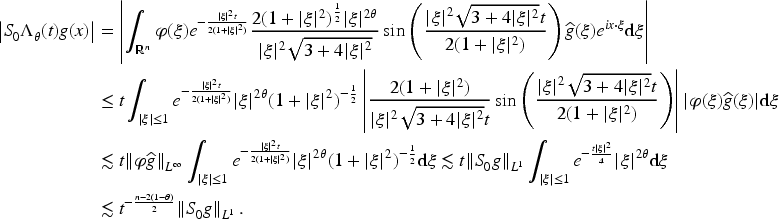
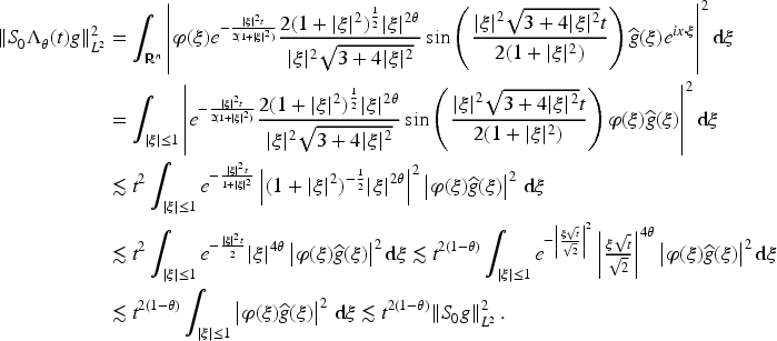
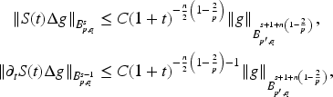
Let $θ \geq 0.$ Consider $s \in R,$ $1 \leq q \leq \infty,$ and $2 \leq p \leq \infty$ with $\frac{1}{p} + \frac{1}{p^{'}} = 1$ . Then, there is a constant $C = C_{n, θ} > 0,$ depending only on $n, θ$ , such that
$‖ Λ_{θ} (t) g ‖_{B_{p, q}^{s}} \leq C t^{- \frac{n}{2} (1 - \frac{2}{p}) + 1 - θ} ‖ g ‖_{B_{p^{'}, q}^{s + n (1 - \frac{2}{p}) - (1 - 2 θ)}},$
(3.1)
for all $g \in B_{p^{'}, q}^{s + n (1 - \frac{2}{p}) - (1 - 2 θ)} (R^{n})$ and $t > 0$ .
Proof.
Using Lemma 3.1 in Banquet et al. (2022) to estimate the integrals $\int_{| ξ | \leq 1} e^{\frac{- | ξ |^{2} t}{4}} | ξ |^{a} d ξ,$ we obtain
$\begin{aligned} | S_{0} Λ_{θ} (t) g (x) | & = | \int_{R^{n}} φ (ξ) e^{- \frac{| ξ |^{2} t}{2 (1 + | ξ |^{2})}} \frac{2 (1 + | ξ |^{2})^{\frac{1}{2}} | ξ |^{2 θ}}{| ξ |^{2} \sqrt{3 + 4 | ξ |^{2}}} \sin (\frac{| ξ |^{2} \sqrt{3 + 4 | ξ |^{2}} t}{2 (1 + | ξ |^{2})}) \hat{g} (ξ) e^{i x \cdot ξ} d ξ | \\ \leq t \int_{| ξ | \leq 1} e^{- \frac{| ξ |^{2} t}{2 (1 + | ξ |^{2})}} | ξ |^{2 θ} (1 + | ξ |^{2})^{- \frac{1}{2}} | \frac{2 (1 + | ξ |^{2})}{| ξ |^{2} \sqrt{3 + 4 | ξ |^{2}} t} \sin (\frac{| ξ |^{2} \sqrt{3 + 4 | ξ |^{2}} t}{2 (1 + | ξ |^{2})}) | | φ (ξ) \hat{g} (ξ) | d ξ \\ ≲ t ‖ φ \hat{g} ‖_{L^{\infty}} \int_{| ξ | \leq 1} e^{- \frac{| ξ |^{2} t}{2 (1 + | ξ |^{2})}} | ξ |^{2 θ} (1 + | ξ |^{2})^{- \frac{1}{2}} d ξ ≲ t ‖ S_{0} g ‖_{L^{1}} \int_{| ξ | \leq 1} e^{- \frac{t | ξ |^{2}}{4}} | ξ |^{2 θ} d ξ \\ ≲ t^{- \frac{n - 2 (1 - θ)}{2}} ‖ S_{0} g ‖_{L^{1}} . \end{aligned}$
Therefore,
$‖ S_{0} Λ_{θ} (t) g ‖_{L^{\infty}} ≲ t^{- \frac{n - 2 (1 - θ)}{2}} ‖ S_{0} g ‖_{L^{1}} .$
(3.2)
On the other hand,
$\begin{aligned} ‖ S_{0} Λ_{θ} (t) g ‖_{L^{2}}^{2} & = \int_{R^{n}} {| φ (ξ) e^{- \frac{| ξ |^{2} t}{2 (1 + | ξ |^{2})}} \frac{2 (1 + | ξ |^{2})^{\frac{1}{2}} | ξ |^{2 θ}}{| ξ |^{2} \sqrt{3 + 4 | ξ |^{2}}} \sin (\frac{| ξ |^{2} \sqrt{3 + 4 | ξ |^{2}} t}{2 (1 + | ξ |^{2})}) \hat{g} (ξ) e^{i x \cdot ξ} |}^{2} d ξ \\ = \int_{| ξ | \leq 1} {| e^{- \frac{| ξ |^{2} t}{2 (1 + | ξ |^{2})}} \frac{2 (1 + | ξ |^{2})^{\frac{1}{2}} | ξ |^{2 θ}}{| ξ |^{2} \sqrt{3 + 4 | ξ |^{2}}} \sin (\frac{| ξ |^{2} \sqrt{3 + 4 | ξ |^{2}} t}{2 (1 + | ξ |^{2})}) φ (ξ) \hat{g} (ξ) |}^{2} d ξ \\ ≲ t^{2} \int_{| ξ | \leq 1} e^{- \frac{| ξ |^{2} t}{1 + | ξ |^{2}}} {| (1 + | ξ |^{2})^{- \frac{1}{2}} | ξ |^{2 θ} |}^{2} {| φ (ξ) \hat{g} (ξ) |}^{2} d ξ \\ ≲ t^{2} \int_{| ξ | \leq 1} e^{- \frac{| ξ |^{2} t}{2}} | ξ |^{4 θ} {| φ (ξ) \hat{g} (ξ) |}^{2} d ξ ≲ t^{2 (1 - θ)} \int_{| ξ | \leq 1} e^{- {| \frac{ξ \sqrt{t}}{\sqrt{2}} |}^{2}} {| \frac{ξ \sqrt{t}}{\sqrt{2}} |}^{4 θ} {| φ (ξ) \hat{g} (ξ) |}^{2} d ξ \\ ≲ t^{2 (1 - θ)} \int_{| ξ | \leq 1} {| φ (ξ) \hat{g} (ξ) |}^{2} d ξ ≲ t^{2 (1 - θ)} ‖ S_{0} g ‖_{L^{2}}^{2} . \end{aligned}$
Thus,
$‖ S_{0} Λ_{θ} (t) g ‖_{L^{2}} ≲ t^{1 - θ} ‖ S_{0} g ‖_{L^{2}} .$
(3.3)
Let $k \geq 1.$ Then $e^{- \frac{| ξ |^{2} t}{2 (1 + | ξ |^{2})}} \leq e^{- \frac{t}{4}},$ if $2^{k - 1} \leq | ξ | \leq 2^{k + 1};$ therefore,
$\begin{aligned} | Δ_{k} Λ_{θ} (t) g (x) | & = | \int_{R^{n}} ψ_{k} (ξ) e^{- \frac{| ξ |^{2} t}{2 (1 + | ξ |^{2})}} \frac{2 (1 + | ξ |^{2})^{\frac{1}{2}} | ξ |^{2 θ}}{| ξ |^{2} \sqrt{3 + 4 | ξ |^{2}}} \sin (\frac{| ξ |^{2} \sqrt{3 + 4 | ξ |^{2}} t}{2 (1 + | ξ |^{2})}) \hat{g} (ξ) e^{i x \cdot ξ} d ξ | \\ \leq \int_{2^{k - 1} \leq | ξ | \leq 2^{k + 1}} e^{- \frac{| ξ |^{2} t}{2 (1 + | ξ |^{2})}} | \frac{2 (1 + | ξ |^{2})^{\frac{1}{2}} | ξ |^{2 θ}}{| ξ |^{2} \sqrt{3 + 4 | ξ |^{2}}} \sin (\frac{| ξ |^{2} \sqrt{3 + 4 | ξ |^{2}} t}{2 (1 + | ξ |^{2})}) ψ_{k} (ξ) \hat{g} (ξ) | d ξ \\ \leq t ‖ ψ_{k} (ξ) \hat{g} ‖_{L^{\infty}} \int_{2^{k - 1} \leq | ξ | \leq 2^{k + 1}} e^{- \frac{| ξ |^{2} t}{2 (1 + | ξ |^{2})}} (1 + | ξ |^{2})^{- \frac{1}{2}} | ξ |^{2 θ} d ξ \\ ≲ t e^{- \frac{t}{4}} ‖ Δ_{k} g ‖_{L^{1}} \int_{2^{k - 1} \leq | ξ | \leq 2^{k + 1}} | ξ |^{2 θ - 1} d ξ ≲ t e^{- \frac{t}{4}} ‖ Δ_{k} g ‖_{L^{1}} \int_{2^{k - 1} \leq | ξ | \leq 2^{k + 1}} 2^{k (2 θ - 1)} d ξ \\ ≲ t e^{- \frac{t}{4}} ‖ Δ_{k} g ‖_{L^{1}} 2^{- k (1 - 2 θ)} 2^{n k} ≲ t e^{- \frac{t}{4}} 2^{n k - k (1 - 2 θ)} ‖ Δ_{k} g ‖_{L^{1}} . \end{aligned}$
Then,
$‖ Δ_{k} Λ_{θ} (t) g ‖_{L^{\infty}} ≲ t e^{- \frac{t}{4}} 2^{n k} 2^{- k (1 - 2 θ)} ‖ Δ_{k} g ‖_{L^{1}} .$
(3.4)

On the other hand,
$\begin{aligned} ‖ Δ_{k} Λ_{θ} (t) g ‖_{L^{2}}^{2} & = \int_{R^{n}} {| ψ_{k} (ξ) e^{- \frac{| ξ |^{2} t}{2 (1 + | ξ |^{2})}} \frac{2 (1 + | ξ |^{2})^{\frac{1}{2}} | ξ |^{2 θ}}{| ξ |^{2} \sqrt{3 + 4 | ξ |^{2}}} \sin (\frac{| ξ |^{2} \sqrt{3 + 4 | ξ |^{2}} t}{2 (1 + | ξ |^{2})}) \hat{g} (ξ) e^{i x \cdot ξ} |}^{2} d ξ \\ = \int_{2^{k - 1} \leq | ξ | \leq 2^{k + 1}} {| e^{- \frac{| ξ |^{2} t}{2 (1 + | ξ |^{2})}} \frac{2 (1 + | ξ |^{2})^{\frac{1}{2}} | ξ |^{2 θ}}{| ξ |^{2} \sqrt{3 + 4 | ξ |^{2}}} \sin (\frac{| ξ |^{2} \sqrt{3 + 4 | ξ |^{2}} t}{2 (1 + | ξ |^{2})}) ψ_{k} (ξ) \hat{g} (ξ) |}^{2} d ξ \\ ≲ t^{2} \int_{2^{k - 1} \leq | ξ | \leq 2^{k + 1}} e^{- \frac{| ξ |^{2} t}{1 + | ξ |^{2}}} (1 + | ξ |^{2})^{- 1} | ξ |^{4 θ} {| ψ_{k} (ξ) \hat{g} (ξ) |}^{2} d ξ \\ ≲ t^{2} \int_{2^{k - 1} \leq | ξ | \leq 2^{k + 1}} e^{- \frac{| ξ |^{2} t}{1 + | ξ |^{2}}} | ξ |^{2 (2 θ - 1)} {| ψ_{k} (ξ) \hat{g} (ξ) |}^{2} d ξ \\ ≲ t^{2} e^{- \frac{t}{2}} \int_{2^{k - 1} \leq | ξ | \leq 2^{k + 1}} 2^{2 k (2 θ - 1)} {| ψ_{k} (ξ) \hat{g} (ξ) |}^{2} d ξ ≲ 2^{- 2 k (1 - 2 θ)} t^{2} e^{- \frac{t}{2}} ‖ Δ_{k} g ‖_{L^{2}}^{2} . \end{aligned}$
Thus,
$‖ Δ_{k} Λ_{θ} (t) g ‖_{L^{2}} ≲ 2^{- k (1 - 2 θ)} t e^{- \frac{t}{4}} ‖ Δ_{k} g ‖_{L^{2}} .$
(3.5)
Taking into account the existence of a constant $C = C_{n, θ} > 0$ such that $t e^{- \frac{t}{4}} \leq C t^{- \frac{n - 2 (1 - θ)}{2}},$ from (3.2) and (3.4), multiplying by $2^{k s}$ and taking the $l^{q} -$ norm, we get
$‖ Λ_{θ} (t) g ‖_{B_{\infty, q}^{s}} ≲ t^{- \frac{n - 2 (1 - θ)}{2}} ‖ g ‖_{B_{1, q}^{s + n - (1 - 2 θ)}} .$
(3.6)
Similarly, considering that $t e^{- \frac{t}{4}} \leq C t^{1 - θ}$ for some positive constant $C = C_{θ},$ from (3.3) and (3.5), multiplying by $2^{k s}$ and taking the $l^{q} -$ norm, we deduce that
$‖ Λ_{θ} (t) g ‖_{B_{2, q}^{s}} ≲ t^{1 - θ} ‖ g ‖_{B_{2, q}^{s - (1 - 2 θ)}} .$
(3.7)
Finally, from complex interpolation (see Bergh & Löfström, 1976, p. 153]), from (3.6) and (3.7) we conclude (3.1).
Lemma 3.2
Let $θ \geq 0$ and $s \in R$ . Assume that $2 \leq p \leq \infty,$ $1 \leq q \leq \infty,$ with $\frac{1}{p} + \frac{1}{p^{'}} = 1$ . Then, there exists a constant $C = C_{θ, n} > 0$ such that
$‖ \partial_{t} Λ_{θ} (t) g ‖_{B_{p, q}^{s - 1}} \leq C t^{- \frac{n}{2} (1 - \frac{2}{p})} ‖ g ‖_{B_{p^{'}, q}^{s - 1 + n (1 - \frac{2}{p}) - (1 - 2 θ)}},$
(3.8)
for all $g \in B_{p^{'}, q}^{s - 1 + n (1 - \frac{2}{p}) - (1 - 2 θ)} (R^{n})$ and $t > 0$ .
Proof.
Using Lemma 3.1 in Banquet et al. (2022) we obtain
$\begin{aligned} | S_{0} \partial_{t} Λ_{θ} (t) g (x) | & \leq | \int_{R^{n}} φ (ξ) e^{- \frac{| ξ |^{2} t}{2 (1 + | ξ |^{2})}} (1 + | ξ |^{2})^{- \frac{1}{2}} | ξ |^{2 θ} \cos (\frac{| ξ |^{2} \sqrt{3 + 4 | ξ |^{2}} t}{2 (1 + | ξ |^{2})}) \hat{g} (ξ) e^{i x \cdot ξ} d ξ | \\ + | \int_{R^{n}} φ (ξ) e^{- \frac{| ξ |^{2} t}{2 (1 + | ξ |^{2})}} \frac{(1 + | ξ |^{2})^{- \frac{1}{2}} | ξ |^{2 θ}}{\sqrt{3 + 4 | ξ |^{2}}} \sin (\frac{| ξ |^{2} \sqrt{3 + 4 | ξ |^{2}} t}{2 (1 + | ξ |^{2})}) \hat{g} (ξ) e^{i x \cdot ξ} d ξ | \\ ≲ ‖ φ \hat{g} ‖_{L^{\infty}} \int_{| ξ | \leq 1} e^{- \frac{| ξ |^{2} t}{2 (1 + | ξ |^{2})}} | ξ |^{2 θ} (1 + | ξ |^{2})^{- \frac{1}{2}} d ξ + ‖ φ \hat{g} ‖_{L^{\infty}} \int_{| ξ | \leq 1} e^{- \frac{| ξ |^{2} t}{2 (1 + | ξ |^{2})}} \frac{(1 + | ξ |^{2})^{- \frac{1}{2}} | ξ |^{2 θ}}{\sqrt{3 + 4 | ξ |^{2}}} d ξ \\ ≲ ‖ φ \hat{g} ‖_{L^{\infty}} \int_{| ξ | \leq 1} e^{- \frac{| ξ |^{2} t}{2 (1 + | ξ |^{2})}} d ξ ≲ ‖ S_{0} g ‖_{L^{1}} \int_{| ξ | \leq 1} e^{- \frac{| ξ |^{2} t}{4}} d ξ ≲ t^{- \frac{n}{2}} ‖ S_{0} g ‖_{L^{1}} . \end{aligned}$
From the last inequality, it follows
$‖ S_{0} \partial_{t} Λ_{θ} (t) g ‖_{L^{\infty}} ≲ t^{- \frac{n}{2}} ‖ S_{0} g ‖_{L^{1}} .$
(3.9)
On the other hand,
$\begin{aligned} ‖ S_{0} \partial_{t} Λ_{θ} (t) g ‖_{L^{2}}^{2} & \leq \int_{R^{n}} {| φ (ξ) e^{- \frac{| ξ |^{2} t}{2 (1 + | ξ |^{2})}} (1 + | ξ |^{2})^{- \frac{1}{2}} | ξ |^{2 θ} \cos (\frac{| ξ |^{2} \sqrt{3 + 4 | ξ |^{2}} t}{2 (1 + | ξ |^{2})}) \hat{g} (ξ) e^{i x \cdot ξ} |}^{2} d ξ \\ + \int_{R^{n}} {| φ (ξ) e^{- \frac{| ξ |^{2} t}{2 (1 + | ξ |^{2})}} \frac{(1 + | ξ |^{2})^{- \frac{1}{2}} | ξ |^{2 θ}}{\sqrt{3 + 4 | ξ |^{2}}} \sin (\frac{| ξ |^{2} \sqrt{3 + 4 | ξ |^{2}} t}{2 (1 + | ξ |^{2})}) φ (ξ) \hat{g} (ξ) e^{i x \cdot ξ} |}^{2} d ξ \\ \leq \int_{| ξ | \leq 1} e^{- \frac{| ξ |^{2} t}{1 + | ξ |^{2}}} ({| (1 + | ξ |^{2})^{- \frac{1}{2}} | ξ |^{2 θ} |}^{2} + {| \frac{(1 + | ξ |^{2})^{- \frac{1}{2}} | ξ |^{2 θ}}{\sqrt{3 + 4 | ξ |^{2}}} |}^{2}) {| φ (ξ) \hat{g} (ξ) |}^{2} d ξ \\ ≲ \int_{| ξ | \leq 1} e^{- \frac{| ξ |^{2} t}{2}} {| φ (ξ) \hat{g} (ξ) |}^{2} d ξ ≲ ‖ S_{0} g ‖_{L^{2}}^{2} . \end{aligned}$
Therefore,
$‖ S_{0} \partial_{t} Λ_{θ} (t) g ‖_{L^{2}} ≲ ‖ S_{0} g ‖_{L^{2}} .$
(3.10)
Now, let $k \geq 1$ an integer. Then
$\begin{aligned} | Δ_{k} \partial_{t} Λ_{θ} (t) g (x) | & \leq \int_{2^{k - 1} \leq | ξ | \leq 2^{k + 1}} e^{- \frac{| ξ |^{2} t}{2 (1 + | ξ |^{2})}} | (1 + | ξ |^{2})^{- \frac{1}{2}} | ξ |^{2 θ} \cos (\frac{| ξ |^{2} \sqrt{3 + 4 | ξ |^{2}} t}{2 (1 + | ξ |^{2})}) ψ_{k} (ξ) \hat{g} (ξ) | d ξ \\ + \int_{2^{k - 1} \leq | ξ | \leq 2^{k + 1}} e^{- \frac{| ξ |^{2} t}{2 (1 + | ξ |^{2})}} | \frac{(1 + | ξ |^{2})^{- \frac{1}{2}} | ξ |^{2 θ}}{\sqrt{3 + 4 | ξ |^{2}}} \sin (\frac{| ξ |^{2} \sqrt{3 + 4 | ξ |^{2}} t}{2 (1 + | ξ |^{2})}) ψ_{k} (ξ) \hat{g} (ξ) | d ξ \\ \leq ‖ ψ_{k} \hat{g} ‖_{L^{\infty}} \int_{2^{k - 1} \leq | ξ | \leq 2^{k + 1}} e^{- \frac{| ξ |^{2} t}{2 (1 + | ξ |^{2})}} (1 + | ξ |^{2})^{- \frac{1}{2}} | ξ |^{2 θ} (1 + \frac{1}{\sqrt{3 + 4 | ξ |^{2}}}) d ξ \\ ≲ e^{- \frac{t}{4}} ‖ Δ_{k} g ‖_{L^{1}} \int_{2^{k - 1} \leq | ξ | \leq 2^{k + 1}} | ξ |^{2 θ - 1} d ξ + e^{- \frac{t}{4}} ‖ Δ_{k} g ‖_{L^{1}} \int_{2^{k - 1} \leq | ξ | \leq 2^{k + 1}} | ξ |^{2 (θ - 1)} d ξ \\ ≲ e^{- \frac{t}{4}} ‖ Δ_{k} g ‖_{L^{1}} \int_{2^{k - 1} \leq | ξ | \leq 2^{k + 1}} 2^{k (2 θ - 1)} d ξ ≲ e^{- \frac{t}{4}} 2^{- k (1 - 2 θ)} 2^{n k} ‖ Δ_{k} g ‖_{L^{1}} . \end{aligned}$
This gives
$‖ Δ_{k} \partial_{t} Λ_{θ} (t) g ‖_{L^{\infty}} ≲ e^{- \frac{t}{4}} 2^{- k (1 - 2 θ)} 2^{n k} ‖ Δ_{k} g ‖_{L^{1}} .$
(3.11)
On the other hand,
$\begin{aligned} ‖ Δ_{k} \partial_{t} Λ_{θ} (t) g ‖_{L^{2}}^{2} & \leq \int_{R^{n}} {| ψ_{k} (ξ) e^{- \frac{| ξ |^{2} t}{2 (1 + | ξ |^{2})}} (1 + | ξ |^{2})^{- \frac{1}{2}} | ξ |^{2 θ} \cos (\frac{| ξ |^{2} \sqrt{3 + 4 | ξ |^{2}} t}{2 (1 + | ξ |^{2})}) \hat{g} (ξ) e^{i x \cdot ξ} |}^{2} d ξ \\ + \int_{R^{n}} {| ψ_{k} (ξ) e^{- \frac{| ξ |^{2} t}{2 (1 + | ξ |^{2})}} \frac{(1 + | ξ |^{2})^{- \frac{1}{2}} | ξ |^{2 θ}}{\sqrt{3 + 4 | ξ |^{2}}} \sin (\frac{| ξ |^{2} \sqrt{3 + 4 | ξ |^{2}} t}{2 (1 + | ξ |^{2})}) \hat{g} (ξ) e^{i x \cdot ξ} |}^{2} d ξ \\ ≲ \int_{2^{k - 1} \leq | ξ | \leq 2^{k + 1}} e^{- \frac{| ξ |^{2} t}{1 + | ξ |^{2}}} (1 + | ξ |^{2})^{- 1} | ξ |^{4 θ} (1 + \frac{1}{3 + 4 | ξ |^{2}}) {| ψ_{k} (ξ) \hat{g} (ξ) |}^{2} d ξ \\ ≲ \int_{2^{k - 1} \leq | ξ | \leq 2^{k + 1}} e^{- \frac{| ξ |^{2} t}{1 + | ξ |^{2}}} | ξ |^{2 (2 θ - 1)} {| ψ_{k} (ξ) \hat{g} (ξ) |}^{2} d ξ + \int_{2^{k - 1} \leq | ξ | \leq 2^{k + 1}} e^{- \frac{| ξ |^{2} t}{1 + | ξ |^{2}}} | ξ |^{4 (θ - 1)} {| ψ_{k} (ξ) \hat{g} (ξ) |}^{2} d ξ \\ ≲ \int_{2^{k - 1} \leq | ξ | \leq 2^{k + 1}} e^{- \frac{| ξ |^{2} t}{1 + | ξ |^{2}}} | ξ |^{2 (2 θ - 1)} {| ψ_{k} (ξ) \hat{g} (ξ) |}^{2} d ξ ≲ e^{- \frac{t}{2}} \int_{2^{k - 1} \leq | ξ | \leq 2^{k + 1}} 2^{2 k (2 θ - 1)} {| ψ_{k} (ξ) \hat{g} (ξ) |}^{2} d ξ \\ ≲ e^{- \frac{t}{2}} 2^{- 2 k (1 - 2 θ)} ‖ Δ_{k} g ‖_{L^{2}}^{2} . \end{aligned}$
From the last inequality, we obtain
$‖ Δ_{k} \partial_{t} Λ_{θ} (t) g ‖_{L^{2}} ≲ e^{- \frac{t}{4}} 2^{- k (1 - 2 θ)} ‖ Δ_{k} g ‖_{L^{2}} .$
(3.12)
Since $e^{- \frac{t}{4}} \leq C t^{- \frac{n}{2}}$ for some $C = C_{n, θ} > 0,$ from (3.9) and (3.11), multiplying by $2^{k (s - 1)}$ and taking the $l^{q} -$ norm, we arrive at
$‖ \partial_{t} Λ_{θ} (t) g ‖_{B_{\infty, q}^{s - 1}} ≲ t^{- \frac{n}{2}} ‖ g ‖_{B_{1, q}^{s - 1 + n - (1 - 2 θ)}} .$
(3.13)
Similarly, from (3.10) for all $t > 0$ and (3.12), multiplying by $2^{k (s - 1)}$ and taking the $l^{q} -$ norm, we have
$‖ \partial_{t} Λ_{θ} (t) g ‖_{B_{2, q}^{s - 1}} ≲ ‖ g ‖_{B_{1, q}^{s - 1 - (1 - 2 θ)}} .$
(3.14)
Finally, using complex interpolation (see Bergh & Löfström, 1976 p. 153), from (3.13) and (3.14) we conclude (3.8).
Lemma 3.3
Let $θ \in [\frac{1}{2}, 1]$ if $n = 1,$ or $θ \in [0, 1]$ if $n \geq 2,$ $s \in R,$ and assume that $2 \leq p \leq \infty$ and $1 \leq q \leq \infty$ . Then, there exists $C > 0$ such that
$‖ Λ_{θ} (t) g ‖_{B_{p, q}^{s}} \leq C (1 + t)^{- (n / 2) (1 - (2 / p)) + (1 - θ)} ‖ g ‖_{B_{p^{'}, q}^{s + n (1 - \frac{2}{p}) - 2 (1 - θ)}},$
(3.15)
for all $g \in B_{p^{'}, q}^{s + n (1 - \frac{2}{p}) - 2 (1 - θ)} (R^{n})$ and $t > 0$ .
Proof.
Note that
$\begin{aligned} | S_{0} Λ_{θ} (t) g (x) | & \leq \int_{| ξ | \leq 1} e^{- \frac{| ξ |^{2} t}{2 (1 + | ξ |^{2})}} | \frac{2 (1 + | ξ |^{2})^{\frac{1}{2}} | ξ |^{2 θ}}{| ξ |^{2} \sqrt{3 + 4 | ξ |^{2}}} \sin (\frac{| ξ |^{2} \sqrt{3 + 4 | ξ |^{2}} t}{2 (1 + | ξ |^{2})}) φ (ξ) \hat{g} (ξ) | d ξ \\ \leq \int_{| ξ | \leq 1} e^{- \frac{| ξ |^{2} t}{2 (1 + | ξ |^{2})}} t | ξ |^{2 θ} (1 + | ξ |^{2})^{- \frac{1}{2}} | \frac{2 (1 + | ξ |^{2})}{| ξ |^{2} \sqrt{3 + 4 | ξ |^{2}} t} \sin (\frac{| ξ |^{2} \sqrt{3 + 4 | ξ |^{2}} t}{2 (1 + | ξ |^{2})}) | | φ (ξ) \hat{g} (ξ) | d ξ \\ ≲ t ‖ φ \hat{g} ‖_{L^{\infty}} \int_{| ξ | \leq 1} e^{- \frac{| ξ |^{2} t}{2 (1 + | ξ |^{2})}} | ξ |^{2 θ} (1 + | ξ |^{2})^{- \frac{1}{2}} d ξ ≲ t ‖ S_{0} g ‖_{L^{1}} \int_{| ξ | \leq 1} e^{- \frac{t | ξ |^{2}}{4}} | ξ |^{2 θ} d ξ \\ ≲ t \cdot t^{- \frac{n + 2 θ}{2}} ‖ S_{0} g ‖_{L^{1}} ≲ t^{- \frac{n - 2 (1 - θ)}{2}} ‖ S_{0} g ‖_{L^{1}} . \end{aligned}$
Thus,
$‖ S_{0} Λ_{θ} (t) g ‖_{L^{\infty}} ≲ t^{- (n - 2 (1 - θ)) / 2} ‖ S_{0} g ‖_{L^{1}} .$
(3.16)
Moreover,
$\begin{aligned} | S_{0} Λ_{θ} (t) g (x) | & \leq \int_{| ξ | \leq 1} e^{- \frac{| ξ |^{2} t}{2 (1 + | ξ |^{2})}} | \frac{2 (1 + | ξ |^{2})^{(\frac{1}{2})} | ξ |^{2 θ}}{| ξ |^{2} \sqrt{3 + 4 | ξ |^{2}}} \sin (\frac{| ξ |^{2} \sqrt{3 + 4 | ξ |^{2}} t}{2 (1 + | ξ |^{2})}) φ (ξ) \hat{g} (ξ) | d ξ \\ \leq \int_{| ξ | \leq 1} e^{- \frac{| ξ |^{2} t}{2 (1 + | ξ |^{2})}} t | ξ |^{2 θ} (1 + | ξ |^{2})^{- \frac{1}{2}} | φ (ξ) \hat{g} (ξ) | d ξ \\ ≲ t ‖ φ \hat{g} ‖_{L^{\infty}} \int_{| ξ | \leq 1} | ξ |^{2 θ} d ξ ≲ t ‖ S_{0} g ‖_{L^{1}} . \end{aligned}$
That is,
$‖ S_{0} Λ_{θ} (t) g ‖_{L^{\infty}} ≲ t ‖ S_{0} g ‖_{L^{1}} .$
(3.17)
Notice that in the case $t > 1$ , since $n - 2 (1 - θ) \geq 0$ , it follows
$t^{- \frac{n - 2 (1 - θ)}{2}} = (2 t)^{- \frac{n - 2 (1 - θ)}{2}} 2^{\frac{n - 2 (1 - θ)}{2}} = (t + t)^{- \frac{n - 2 (1 - θ)}{2}} 2^{\frac{n - 2 (1 - θ)}{2}} \leq (1 + t)^{- \frac{n - 2 (1 - θ)}{2}} 2^{\frac{n - 2 (1 - θ)}{2}},$
(3.18)
and, in the case $t \leq 1$ , we have
$\begin{aligned} t & \leq 1 = 2^{\frac{n - 2 (1 - θ)}{2}} 2^{- \frac{n - 2 (1 - θ)}{2}} = 2^{\frac{n - 2 (1 - θ)}{2}} (1 + 1)^{- \frac{n - 2 (1 - θ)}{2}} \leq 2^{\frac{n - 2 (1 - θ)}{2}} (1 + t)^{- \frac{n - 2 (1 - θ)}{2}} ≲ (1 + t)^{- \frac{n - 2 (1 - θ)}{2}} . \end{aligned}$
(3.19)
From (3.16) and (3.18), and from (3.17) and (3.19) we have that for all $t > 0$ , it follows
$‖ S_{0} Λ_{θ} (t) g ‖_{L^{\infty}} ≲ (1 + t)^{- \frac{n - 2 (1 - θ)}{2}} ‖ S_{0} g ‖_{L^{1}} .$
(3.20)
On the other hand,
$\begin{aligned} ‖ S_{0} Λ_{θ} (t) g ‖_{L^{2}}^{2} & \leq \int_{| ξ | \leq 1} {| e^{- \frac{| ξ |^{2} t}{2 (1 + | ξ |^{2})}} \frac{2 (1 + | ξ |^{2})^{\frac{1}{2}} | ξ |^{2 θ}}{| ξ |^{2} \sqrt{3 + 4 | ξ |^{2}}} \sin (\frac{| ξ |^{2} \sqrt{3 + 4 | ξ |^{2}} t}{2 (1 + | ξ |^{2})}) φ (ξ) \hat{g} (ξ) |}^{2} d ξ \\ ≲ t^{2} \int_{| ξ | \leq 1} e^{- \frac{| ξ |^{2} t}{1 + | ξ |^{2}}} {| (1 + | ξ |^{2})^{- \frac{1}{2}} | ξ |^{2 θ} |}^{2} {| φ (ξ) \hat{g} (ξ) |}^{2} d ξ \\ ≲ t^{2} \int_{| ξ | \leq 1} e^{- \frac{| ξ |^{2} t}{2}} | ξ |^{4 θ} {| φ (ξ) \hat{g} (ξ) |}^{2} d ξ ≲ t^{2 (1 - θ)} \int_{| ξ | \leq 1} e^{- {| \frac{ξ \sqrt{t}}{\sqrt{2}} |}^{2}} {| \frac{ξ \sqrt{t}}{\sqrt{2}} |}^{4 θ} {| φ (ξ) \hat{g} (ξ) |}^{2} d ξ \\ ≲ t^{2 (1 - θ)} \int_{| ξ | \leq 1} {| φ (ξ) \hat{g} (ξ) |}^{2} d ξ ≲ t^{2 (1 - θ)} ‖ S_{0} g ‖_{L^{2}}^{2} . \end{aligned}$
Thus, $‖ S_{0} Λ_{θ} (t) g ‖_{L^{2}} ≲ t^{1 - θ} ‖ S_{0} g ‖_{L^{2}} .$ In this case, since that $1 - θ \geq 0,$ it holds $t^{1 - θ} \leq (1 + t)^{1 - θ},$ and therefore,
$‖ S_{0} Λ_{θ} (t) g ‖_{L^{2}} ≲ (1 + t)^{1 - θ} ‖ S_{0} g ‖_{L^{2}} .$
(3.21)
Now, let $k \geq 1$ . Notice that $e^{- \frac{| ξ |^{2} t}{2 (1 + | ξ |^{2})}} \leq e^{- \frac{t}{4}},$ if $2^{k - 1} \leq | ξ | \leq 2^{k + 1} .$ Therefore,
$\begin{aligned} | Δ_{k} Λ_{θ} (t) g (x) | & \leq \int_{2^{k - 1} \leq | ξ | \leq 2^{k + 1}} e^{- \frac{| ξ |^{2} t}{2 (1 + | ξ |^{2})}} | \frac{2 (1 + | ξ |^{2})^{\frac{1}{2}} | ξ |^{2 θ}}{| ξ |^{2} \sqrt{3 + 4 | ξ |^{2}}} \sin (\frac{| ξ |^{2} \sqrt{3 + 4 | ξ |^{2}} t}{2 (1 + | ξ |^{2})}) ψ_{k} (ξ) \hat{g} (ξ) | d ξ \\ ≲ ‖ ψ_{k} (ξ) \hat{g} ‖_{L^{\infty}} \int_{2^{k - 1} \leq | ξ | \leq 2^{k + 1}} e^{- \frac{| ξ |^{2} t}{2 (1 + | ξ |^{2})}} \frac{(1 + | ξ |^{2})^{\frac{1}{2}} | ξ |^{2 (θ - 1)}}{\sqrt{3 + 4 | ξ |^{2}}} d ξ \\ ≲ e^{- \frac{t}{4}} ‖ Δ_{k} g ‖_{L^{1}} \int_{2^{k - 1} \leq | ξ | \leq 2^{k + 1}} | ξ |^{2 (θ - 1)} d ξ ≲ e^{- \frac{t}{4}} ‖ Δ_{k} g ‖_{L^{1}} \int_{2^{k - 1} \leq | ξ | \leq 2^{k + 1}} 2^{2 k (θ - 1)} d ξ \\ ≲ e^{- \frac{t}{4}} ‖ Δ_{k} g ‖_{L^{1}} 2^{- 2 k (1 - θ)} 2^{n k} ≲ e^{- \frac{t}{4}} 2^{n k - 2 k (1 - θ)} ‖ Δ_{k} g ‖_{L^{1}} . \end{aligned}$
Thus,
$‖ Δ_{k} Λ_{θ} (t) g ‖_{L^{\infty}} ≲ e^{- \frac{t}{4}} 2^{n k} 2^{- 2 k (1 - θ)} ‖ Δ_{k} g ‖_{L^{1}} .$
(3.22)
On the other hand,
$\begin{aligned} ‖ Δ_{k} Λ_{θ} (t) g ‖_{L^{2}}^{2} & \leq \int_{2^{k - 1} \leq | ξ | \leq 2^{k + 1}} {| e^{- \frac{| ξ |^{2} t}{2 (1 + | ξ |^{2})}} \frac{2 (1 + | ξ |^{2})^{\frac{1}{2}} | ξ |^{2 θ}}{| ξ |^{2} \sqrt{3 + 4 | ξ |^{2}}} \sin (\frac{| ξ |^{2} \sqrt{3 + 4 | ξ |^{2}} t}{2 (1 + | ξ |^{2})}) ψ_{k} (ξ) \hat{g} (ξ) |}^{2} d ξ \\ ≲ \int_{2^{k - 1} \leq | ξ | \leq 2^{k + 1}} e^{- \frac{| ξ |^{2} t}{1 + | ξ |^{2}}} | ξ |^{4 (θ - 1)} {| ψ_{k} (ξ) \hat{g} (ξ) |}^{2} d ξ \\ ≲ e^{- \frac{t}{2}} 2^{4 k (θ - 1)} \int_{2^{k - 1} \leq | ξ | \leq 2^{k + 1}} {| ψ_{k} (ξ) \hat{g} (ξ) |}^{2} d ξ ≲ e^{- \frac{t}{2}} 2^{4 k (θ - 1)} ‖ Δ_{k} g ‖_{L^{2}}^{2} . \end{aligned}$
Consequently,
$\begin{aligned} ‖ Δ_{k} Λ_{θ} (t) g ‖_{L^{2}} ≲ 2^{- 2 k (1 - θ)} e^{- \frac{t}{4}} ‖ Δ_{k} g ‖_{L^{2}} . \end{aligned}$
(3.23)
Arguing as in the end of the proof of Lemma 3.1, from (3.20)–(3.23) we can conclude (3.15).
Lemma 3.4
Let $θ \geq 0,$ $s \in R$ , $2 \leq p \leq \infty$ and $1 \leq q \leq \infty$ . Then, there exists a constant $C = C_{n, θ} > 0$ such that
$‖ \partial_{t} Λ_{θ} (t) g ‖_{B_{p, q}^{s - 1}} \leq C (1 + t)^{- \frac{n}{2} (1 - \frac{2}{p}) - θ} ‖ g ‖_{B_{p^{'}, q}^{s + n (1 - \frac{2}{p}) - 2 (1 - θ)}},$
(3.24)
for all $g \in B_{p^{'}, q}^{s + n (1 - \frac{2}{p}) - 2 (1 - θ)} (R^{n})$ and $t > 0$ .
Proof.
Initially, we have
$\begin{aligned} | S_{0} \partial_{t} Λ_{θ} (t) g (x) | & \leq | \int_{R^{n}} φ (ξ) e^{- \frac{| ξ |^{2} t}{2 (1 + | ξ |^{2})}} (1 + | ξ |^{2})^{- \frac{1}{2}} | ξ |^{2 θ} \cos (\frac{| ξ |^{2} \sqrt{3 + 4 | ξ |^{2}} t}{2 (1 + | ξ |^{2})}) \hat{g} (ξ) e^{i x \cdot ξ} d ξ | \\ + | \int_{R^{n}} φ (ξ) e^{- \frac{| ξ |^{2} t}{2 (1 + | ξ |^{2})}} \frac{(1 + | ξ |^{2})^{- \frac{1}{2}} | ξ |^{2 θ}}{\sqrt{3 + 4 | ξ |^{2}}} \sin (\frac{| ξ |^{2} \sqrt{3 + 4 | ξ |^{2}} t}{2 (1 + | ξ |^{2})}) \hat{g} (ξ) e^{i x \cdot ξ} d ξ | \\ ≲ ‖ φ \hat{g} ‖_{L^{\infty}} \int_{| ξ | \leq 1} e^{- \frac{| ξ |^{2} t}{2 (1 + | ξ |^{2})}} | ξ |^{2 θ} (1 + | ξ |^{2})^{- \frac{1}{2}} d ξ + ‖ φ \hat{g} ‖_{L^{\infty}} \int_{| ξ | \leq 1} e^{- \frac{| ξ |^{2} t}{2 (1 + | ξ |^{2})}} \frac{(1 + | ξ |^{2})^{- \frac{1}{2}} | ξ |^{2 θ}}{\sqrt{3 + 4 | ξ |^{2}}} d ξ \\ ≲ ‖ φ \hat{g} ‖_{L^{\infty}} \int_{| ξ | \leq 1} e^{- \frac{| ξ |^{2} t}{2 (1 + | ξ |^{2})}} | ξ |^{2 θ} d ξ ≲ ‖ S_{0} g ‖_{L^{1}} \int_{| ξ | \leq 1} e^{- \frac{| ξ |^{2} t}{4}} | ξ |^{2 θ} d ξ ≲ t^{- \frac{n + 2 θ}{2}} ‖ S_{0} g ‖_{L^{1}} . \end{aligned}$
(3.25)
Thus,
$‖ S_{0} \partial_{t} Λ_{θ} (t) g ‖_{L^{\infty}} ≲ t^{- \frac{n}{2} - θ} ‖ S_{0} g ‖_{L^{1}} .$
(3.26)
Now, notice that
$\int_{| ξ | \leq 1} e^{- \frac{| ξ |^{2} t}{4}} | ξ |^{2 θ} d ξ \leq 1.$
Then, the same argument used in (3.25) allows us to obtain the following estimate
$‖ S_{0} \partial_{t} Λ_{θ} (t) g ‖_{L^{\infty}} ≲ ‖ S_{0} g ‖_{L^{1}},$
(3.27)
and, from (3.26) and (3.27) it follows that
$‖ S_{0} \partial_{t} Λ_{θ} (t) g ‖_{L^{\infty}} ≲ (1 + t)^{- \frac{n}{2} - θ} ‖ S_{0} g ‖_{L^{1}} .$
(3.28)
On the other hand,
$\begin{aligned} ‖ S_{0} \partial_{t} Λ_{θ} (t) g ‖_{L^{2}}^{2} & \leq \int_{R^{n}} {| φ (ξ) e^{- \frac{| ξ |^{2} t}{2 (1 + | ξ |^{2})}} (1 + | ξ |^{2})^{- \frac{1}{2}} | ξ |^{2 θ} \cos (\frac{| ξ |^{2} \sqrt{3 + 4 | ξ |^{2}} t}{2 (1 + | ξ |^{2})}) \hat{g} (ξ) e^{i x \cdot ξ} |}^{2} d ξ \\ + \int_{R^{n}} {| φ (ξ) e^{- \frac{| ξ |^{2} t}{2 (1 + | ξ |^{2})}} \frac{(1 + | ξ |^{2})^{- \frac{1}{2}} | ξ |^{2 θ}}{\sqrt{3 + 4 | ξ |^{2}}} \sin (\frac{| ξ |^{2} \sqrt{3 + 4 | ξ |^{2}} t}{2 (1 + | ξ |^{2})}) φ (ξ) \hat{g} (ξ) e^{i x \cdot ξ} |}^{2} d ξ \\ \leq \int_{| ξ | \leq 1} e^{- \frac{| ξ |^{2} t}{1 + | ξ |^{2}}} {| (1 + | ξ |^{2})^{- \frac{1}{2}} | ξ |^{2 θ} |}^{2} {| φ (ξ) \hat{g} (ξ) |}^{2} d ξ \\ + \int_{| ξ | \leq 1} e^{- \frac{| ξ |^{2} t}{1 + | ξ |^{2}}} {| \frac{(1 + | ξ |^{2})^{- \frac{1}{2}} | ξ |^{2 θ}}{\sqrt{3 + 4 | ξ |^{2}}} |}^{2} {| φ (ξ) \hat{g} (ξ) |}^{2} d ξ \\ \leq \int_{| ξ | \leq 1} e^{- \frac{| ξ |^{2} t}{1 + | ξ |^{2}}} (1 + | ξ |^{2})^{- 1} | ξ |^{4 θ} {| φ (ξ) \hat{g} (ξ) |}^{2} d ξ + \int_{| ξ | \leq 1} e^{- \frac{| ξ |^{2} t}{1 + | ξ |^{2}}} \frac{(1 + | ξ |^{2})^{- 1} | ξ |^{4 θ}}{3 + 4 | ξ |^{2}} {| φ (ξ) \hat{g} (ξ) |}^{2} d ξ \\ ≲ \int_{| ξ | \leq 1} e^{- \frac{| ξ |^{2} t}{2}} | ξ |^{4 θ} {| φ (ξ) \hat{g} (ξ) |}^{2} d ξ ≲ t^{- 2 θ} \int_{| ξ | \leq 1} {| φ (ξ) \hat{g} (ξ) |}^{2} d ξ ≲ t^{- 2 θ} ‖ S_{0} g ‖_{L^{2}}^{2} . \end{aligned}$
(3.29)
Thus,
$‖ S_{0} \partial_{t} Λ_{θ} (t) g ‖_{L^{2}} ≲ t^{- θ} ‖ S_{0} g ‖_{L^{2}} .$
(3.30)
Moreover, using that, if $| ξ | \leq 1$ then $e^{- \frac{| ξ |^{2} t}{2}} | ξ |^{4 θ} \leq 1,$ arguing as in (3.29) we can get
$‖ S_{0} \partial_{t} Λ_{θ} (t) g ‖_{L^{2}} ≲ ‖ S_{0} g ‖_{L^{2}} .$
(3.31)
Then, from (3.30) and (3.31) we obtain
$‖ S_{0} \partial_{t} Λ_{θ} (t) g ‖_{L^{2}} ≲ (1 + t)^{- θ} ‖ S_{0} g ‖_{L^{2}} .$
(3.32)
Now, let $k \geq 1$ an integer. Then,
$\begin{aligned} | Δ_{k} \partial_{t} Λ_{θ} (t) g (x) | & \leq \int_{2^{k - 1} \leq | ξ | \leq 2^{k + 1}} e^{- \frac{| ξ |^{2} t}{2 (1 + | ξ |^{2})}} | (1 + | ξ |^{2})^{- \frac{1}{2}} | ξ |^{2 θ} \cos (\frac{| ξ |^{2} \sqrt{3 + 4 | ξ |^{2}} t}{2 (1 + | ξ |^{2})}) ψ_{k} (ξ) \hat{g} (ξ) | d ξ \\ + \int_{2^{k - 1} \leq | ξ | \leq 2^{k + 1}} e^{- \frac{| ξ |^{2} t}{2 (1 + | ξ |^{2})}} | \frac{(1 + | ξ |^{2})^{- \frac{1}{2}} | ξ |^{2 θ}}{\sqrt{3 + 4 | ξ |^{2}}} \sin (\frac{| ξ |^{2} \sqrt{3 + 4 | ξ |^{2}} t}{2 (1 + | ξ |^{2})}) ψ_{k} (ξ) \hat{g} (ξ) | d ξ \\ \leq ‖ ψ_{k} \hat{g} ‖_{L^{\infty}} \int_{2^{k - 1} \leq | ξ | \leq 2^{k + 1}} e^{- \frac{| ξ |^{2} t}{2 (1 + | ξ |^{2})}} (1 + | ξ |^{2})^{- \frac{1}{2}} | ξ |^{2 θ} d ξ \\ + ‖ ψ_{k} \hat{g} ‖_{L^{\infty}} \int_{2^{k - 1} \leq | ξ | \leq 2^{k + 1}} e^{- \frac{| ξ |^{2} t}{2 (1 + | ξ |^{2})}} \frac{(1 + | ξ |^{2})^{- \frac{1}{2}} | ξ |^{2 θ}}{\sqrt{3 + 4 | ξ |^{2}}} d ξ \\ ≲ e^{- \frac{t}{4}} ‖ Δ_{k} g ‖_{L^{1}} \int_{2^{k - 1} \leq | ξ | \leq 2^{k + 1}} | ξ |^{2 θ - 1} d ξ + e^{- \frac{t}{4}} ‖ Δ_{k} g ‖_{L^{1}} \int_{2^{k - 1} \leq | ξ | \leq 2^{k + 1}} | ξ |^{2 (θ - 1)} d ξ \\ ≲ e^{- \frac{t}{4}} ‖ Δ_{k} g ‖_{L^{1}} \int_{2^{k - 1} \leq | ξ | \leq 2^{k + 1}} 2^{k (2 θ - 1)} d ξ ≲ e^{- \frac{t}{4}} 2^{- k (1 - 2 θ)} 2^{n k} ‖ Δ_{k} g ‖_{L^{1}} . \end{aligned}$
Thus,
$‖ Δ_{k} \partial_{t} Λ_{θ} (t) g ‖_{L^{\infty}} ≲ e^{- \frac{t}{4}} 2^{n k} 2^{- k (1 - 2 θ)} ‖ Δ_{k} g ‖_{L^{1}} .$
(3.33)
On the other hand,
$\begin{aligned} ‖ Δ_{k} \partial_{t} Λ_{θ} (t) g ‖_{L^{2}}^{2} & \leq \int_{R^{n}} {| ψ_{k} (ξ) e^{- \frac{| ξ |^{2} t}{2 (1 + | ξ |^{2})}} (1 + | ξ |^{2})^{- \frac{1}{2}} | ξ |^{2 θ} \cos (\frac{| ξ |^{2} \sqrt{3 + 4 | ξ |^{2}} t}{2 (1 + | ξ |^{2})}) \hat{g} (ξ) e^{i x \cdot ξ} |}^{2} d ξ \\ + \int_{R^{n}} {| ψ_{k} (ξ) e^{- \frac{| ξ |^{2} t}{2 (1 + | ξ |^{2})}} \frac{(1 + | ξ |^{2})^{- \frac{1}{2}} | ξ |^{2 θ}}{\sqrt{3 + 4 | ξ |^{2}}} \sin (\frac{| ξ |^{2} \sqrt{3 + 4 | ξ |^{2}} t}{2 (1 + | ξ |^{2})}) \hat{g} (ξ) e^{i x \cdot ξ} |}^{2} d ξ \\ ≲ \int_{2^{k - 1} \leq | ξ | \leq 2^{k + 1}} e^{- \frac{| ξ |^{2} t}{1 + | ξ |^{2}}} (1 + | ξ |^{2})^{- 1} | ξ |^{4 θ} {| ψ_{k} (ξ) \hat{g} (ξ) |}^{2} d ξ \\ + \int_{2^{k - 1} \leq | ξ | \leq 2^{k + 1}} e^{- \frac{| ξ |^{2} t}{1 + | ξ |^{2}}} \frac{(1 + | ξ |^{2})^{- 1} | ξ |^{4 θ}}{3 + 4 | ξ |^{2}} {| ψ_{k} (ξ) \hat{g} (ξ) |}^{2} d ξ \\ ≲ \int_{2^{k - 1} \leq | ξ | \leq 2^{k + 1}} e^{- \frac{| ξ |^{2} t}{1 + | ξ |^{2}}} | ξ |^{2 (2 θ - 1)} {| ψ_{k} (ξ) \hat{g} (ξ) |}^{2} d ξ + \int_{2^{k - 1} \leq | ξ | \leq 2^{k + 1}} e^{- \frac{| ξ |^{2} t}{1 + | ξ |^{2}}} | ξ |^{4 (θ - 1)} {| ψ_{k} (ξ) \hat{g} (ξ) |}^{2} d ξ \\ ≲ \int_{2^{k - 1} \leq | ξ | \leq 2^{k + 1}} e^{- \frac{| ξ |^{2} t}{1 + | ξ |^{2}}} | ξ |^{2 (2 θ - 1)} {| ψ_{k} (ξ) \hat{g} (ξ) |}^{2} d ξ ≲ e^{- \frac{t}{2}} \int_{2^{k - 1} \leq | ξ | \leq 2^{k + 1}} 2^{2 k (2 θ - 1)} {| ψ_{k} (ξ) \hat{g} (ξ) |}^{2} d ξ \\ ≲ e^{- \frac{t}{2}} 2^{- 2 k (1 - 2 θ)} ‖ Δ_{k} g ‖_{L^{2}}^{2} . \end{aligned}$
Thus,
$‖ Δ_{k} \partial_{t} Λ_{θ} (t) g ‖_{L^{2}} ≲ e^{- \frac{t}{4}} 2^{- k (1 - 2 θ)} ‖ Δ_{k} g ‖_{L^{2}} .$
(3.34)
Since there exists a constant $C = C_{n, θ}$ such that $e^{- \frac{t}{4}} \leq C (1 + t)^{- \frac{n}{2} - θ},$ from (3.28) and (3.33), multiplying by $2^{k (s - 1)}$ and taking the $l^{q} -$ norm, we get
$‖ \partial_{t} Λ_{θ} (t) g ‖_{B_{\infty, q}^{s - 1}} ≲ (1 + t)^{- \frac{n}{2} - θ} ‖ g ‖_{B_{1, q}^{s - 1 + n - (1 - 2 θ)}} .$
(3.35)
Similarly, since $e^{- \frac{t}{4}} \leq C (1 + t)^{- θ}$ for some $C = C_{n, θ} > 0,$ from (3.30) and (3.34), multiplying by $2^{k (s - 1)}$ and adding we get
$‖ \partial_{t} Λ_{θ} (t) g ‖_{B_{2, q}^{s - 1}} ≲ (1 + t)^{- θ} ‖ g ‖_{B_{1, q}^{s - 1 - (1 - 2 θ)}} .$
(3.36)
Finally, from complex interpolation (see Bergh & Löfström, 1976), from (3.35) and (3.36) we arrive at (3.24).
Lemma 3.5
Let $θ \geq 0$ , $s \in R,$ $2 \leq p \leq \infty$ and $1 \leq q \leq \infty$ . Then, there exists a constant $C = C_{n, θ} > 0$ such that
$‖ \partial_{t}^{2} Λ_{θ} (t) g ‖_{B_{p, q}^{s - 1}} \leq C (1 + t)^{- \frac{n}{2} (1 - \frac{2}{p}) - (θ + 1)} ‖ g ‖_{B_{p^{'}, q}^{s + n (1 - \frac{2}{p}) - 1 + 2 θ}}$
(3.37)
for all $g \in B_{p^{'}, q}^{s + n (1 - \frac{2}{p}) - 1 + 2 θ} (R^{n})$ and $t > 0$ .
Proof.
Initially we have
$\begin{aligned} | S_{0} \partial_{t}^{2} Λ_{θ} (t) g (x) | & \leq | \int_{R^{n}} φ (ξ) e^{- \frac{| ξ |^{2} t}{2 (1 + | ξ |^{2})}} \frac{| ξ |^{2 (θ + 1)}}{(1 + | ξ |^{2})^{\frac{3}{2}}} \cos (\frac{| ξ |^{2} \sqrt{3 + 4 | ξ |^{2}} t}{2 (1 + | ξ |^{2})}) \hat{g} (ξ) e^{i x \cdot ξ} d ξ | \\ + | \int_{R^{n}} φ (ξ) e^{- \frac{| ξ |^{2} t}{2 (1 + | ξ |^{2})}} \frac{| ξ |^{2 (θ + 1)} (1 + 2 | ξ |^{2})}{(1 + | ξ |^{2})^{\frac{3}{2}} \sqrt{3 + 4 | ξ |^{2}}} \sin (\frac{| ξ |^{2} \sqrt{3 + 4 | ξ |^{2}} t}{2 (1 + | ξ |^{2})}) \hat{g} (ξ) e^{i x \cdot ξ} d ξ | \\ ≲ ‖ φ \hat{g} ‖_{L^{\infty}} \int_{| ξ | \leq 1} e^{- \frac{| ξ |^{2} t}{2 (1 + | ξ |^{2})}} \frac{| ξ |^{2 (θ + 1)}}{(1 + | ξ |^{2})^{\frac{3}{2}}} d ξ + ‖ φ \hat{g} ‖_{L^{\infty}} \int_{| ξ | \leq 1} e^{- \frac{| ξ |^{2} t}{2 (1 + | ξ |^{2})}} \frac{| ξ |^{2 (θ + 1)} (1 + 2 | ξ |^{2})}{(1 + | ξ |^{2})^{\frac{3}{2}} \sqrt{3 + 4 | ξ |^{2}}} d ξ \\ ≲ ‖ φ \hat{g} ‖_{L^{\infty}} \int_{| ξ | \leq 1} e^{- \frac{| ξ |^{2} t}{2 (1 + | ξ |^{2})}} | ξ |^{2 (θ + 1)} d ξ ≲ ‖ S_{0} g ‖_{L^{1}} \int_{| ξ | \leq 1} e^{- \frac{| ξ |^{2} t}{4}} | ξ |^{2 (θ + 1)} d ξ \\ ≲ t^{- \frac{n}{2} - (θ + 1)} ‖ S_{0} g ‖_{L^{1}} . \end{aligned}$
(3.38)
Therefore,
$‖ S_{0} \partial_{t}^{2} Λ_{θ} (t) g ‖_{L^{\infty}} ≲ t^{- \frac{n}{2} - (θ + 1)} ‖ S_{0} g ‖_{L^{1}} .$
(3.39)
Moreover, since
$\int_{| ξ | \leq 1} e^{- \frac{| ξ |^{2} t}{4}} | ξ |^{2 (θ + 1)} d ξ \leq 1,$
the same argument used in (3.38), allow us to obtain
$‖ S_{0} \partial_{t}^{2} Λ_{θ} (t) g ‖_{L^{\infty}} ≲ ‖ S_{0} g ‖_{L^{1}},$
(3.40)
and from (3.39) and (3.40) it follows that
$‖ S_{0} \partial_{t}^{2} Λ_{θ} (t) g ‖_{L^{\infty}} ≲ (1 + t)^{- \frac{n}{2} - (θ + 1)} ‖ S_{0} g ‖_{L^{1}} .$
On the other hand,
$\begin{aligned} ‖ S_{0} \partial_{t}^{2} Λ_{θ} (t) g ‖_{L^{2}}^{2} & \leq \int_{| ξ | \leq 1} e^{- \frac{| ξ |^{2} t}{1 + | ξ |^{2}}} {| \frac{| ξ |^{2 (θ + 1)}}{(1 + | ξ |^{2})^{\frac{3}{2}}} |}^{2} {| φ (ξ) \hat{g} (ξ) |}^{2} d ξ \\ + \int_{| ξ | \leq 1} e^{- \frac{| ξ |^{2} t}{1 + | ξ |^{2}}} {| \frac{| ξ |^{2 (θ + 1)} (1 + 2 | ξ |^{2})}{(1 + | ξ |^{2})^{\frac{3}{2}} \sqrt{3 + 4 | ξ |^{2}}} |}^{2} {| φ (ξ) \hat{g} (ξ) |}^{2} d ξ \\ \leq \int_{| ξ | \leq 1} e^{- \frac{| ξ |^{2} t}{1 + | ξ |^{2}}} \frac{| ξ |^{4 (θ + 1)}}{(1 + | ξ |^{2})^{3}} {| φ (ξ) \hat{g} (ξ) |}^{2} d ξ + \int_{| ξ | \leq 1} e^{- \frac{| ξ |^{2} t}{1 + | ξ |^{2}}} \frac{| ξ |^{4 (θ + 1)} (1 + 2 | ξ |^{2})^{2}}{(1 + | ξ |^{2})^{3} (3 + 4 | ξ |^{2})} {| φ (ξ) \hat{g} (ξ) |}^{2} d ξ \\ ≲ \int_{| ξ | \leq 1} e^{- \frac{| ξ |^{2} t}{2}} | ξ |^{4 (θ + 1)} {| φ (ξ) \hat{g} (ξ) |}^{2} d ξ ≲ t^{- 2 (θ + 1)} ‖ S_{0} g ‖_{L^{2}}^{2} . \end{aligned}$
(3.41)
Thus,
$‖ S_{0} \partial_{t}^{2} Λ_{θ} (t) g ‖_{L^{2}} ≲ t^{- (θ + 1)} ‖ S_{0} g ‖_{L^{2}} .$
(3.42)
Moreover, since that $e^{- \frac{| ξ |^{2} t}{2}} | ξ |^{4 (θ + 1)} \leq 1,$ provided $| ξ | \leq 1,$ arguing as in (3.41) we also have
$‖ S_{0} \partial_{t}^{2} Λ_{θ} (t) g ‖_{L^{2}} ≲ ‖ S_{0} g ‖_{L^{2}},$
(3.43)
which implies
$‖ S_{0} \partial_{t}^{2} Λ_{θ} (t) g ‖_{L^{2}} ≲ (1 + t)^{- (θ + 1)} ‖ S_{0} g ‖_{L^{2}} .$
(3.44)
Now, let $k \geq 1$ an integer. Then,
$\begin{aligned} | Δ_{k} \partial_{t}^{2} Λ_{θ} (t) g (x) | & \leq | \int_{R^{n}} ψ_{k} (ξ) e^{- \frac{| ξ |^{2} t}{2 (1 + | ξ |^{2})}} \frac{| ξ |^{2 (θ + 1)}}{(1 + | ξ |^{2})^{\frac{3}{2}}} \cos (\frac{| ξ |^{2} \sqrt{3 + 4 | ξ |^{2}} t}{2 (1 + | ξ |^{2})}) \hat{g} (ξ) e^{i x \cdot ξ} d ξ | \\ + | \int_{R^{n}} ψ_{k} (ξ) e^{- \frac{| ξ |^{2} t}{2 (1 + | ξ |^{2})}} \frac{| ξ |^{2 (θ + 1)} (1 + 2 | ξ |^{2})}{(1 + | ξ |^{2})^{\frac{3}{2}} \sqrt{3 + 4 | ξ |^{2}}} \sin (\frac{| ξ |^{2} \sqrt{3 + 4 | ξ |^{2}} t}{2 (1 + | ξ |^{2})}) \hat{g} (ξ) e^{i x \cdot ξ} d ξ | \\ \leq \int_{2^{k - 1} \leq | ξ | \leq 2^{k + 1}} e^{- \frac{| ξ |^{2} t}{2 (1 + | ξ |^{2})}} | \frac{| ξ |^{2 (θ + 1)}}{(1 + | ξ |^{2})^{\frac{3}{2}}} \cos (\frac{| ξ |^{2} \sqrt{3 + 4 | ξ |^{2}} t}{2 (1 + | ξ |^{2})}) ψ_{k} (ξ) \hat{g} (ξ) | d ξ \\ + \int_{2^{k - 1} \leq | ξ | \leq 2^{k + 1}} e^{- \frac{| ξ |^{2} t}{2 (1 + | ξ |^{2})}} | \frac{| ξ |^{2 (θ + 1)} (1 + 2 | ξ |^{2})}{(1 + | ξ |^{2})^{\frac{3}{2}} \sqrt{3 + 4 | ξ |^{2}}} \sin (\frac{| ξ |^{2} \sqrt{3 + 4 | ξ |^{2}} t}{2 (1 + | ξ |^{2})}) ψ_{k} (ξ) \hat{g} (ξ) | d ξ \\ \leq ‖ ψ_{k} \hat{g} ‖_{L^{\infty}} \int_{2^{k - 1} \leq | ξ | \leq 2^{k + 1}} e^{- \frac{| ξ |^{2} t}{2 (1 + | ξ |^{2})}} \frac{| ξ |^{2 (θ + 1)}}{(1 + | ξ |^{2})^{\frac{3}{2}}} d ξ \\ + ‖ ψ_{k} \hat{g} ‖_{L^{\infty}} \int_{2^{k - 1} \leq | ξ | \leq 2^{k + 1}} e^{- \frac{| ξ |^{2} t}{2 (1 + | ξ |^{2})}} \frac{| ξ |^{2 (θ + 1)} (1 + 2 | ξ |^{2})}{(1 + | ξ |^{2})^{\frac{3}{2}} \sqrt{3 + 4 | ξ |^{2}}} d ξ \\ ≲ e^{- \frac{t}{4}} ‖ Δ_{k} g ‖_{L^{1}} \int_{2^{k - 1} \leq | ξ | \leq 2^{k + 1}} | ξ |^{2 θ - 1} d ξ + e^{- \frac{t}{4}} ‖ Δ_{k} g ‖_{L^{1}} \int_{2^{k - 1} \leq | ξ | \leq 2^{k + 1}} | ξ |^{2 θ} d ξ \\ ≲ e^{- \frac{t}{4}} ‖ Δ_{k} g ‖_{L^{1}} \int_{2^{k - 1} \leq | ξ | \leq 2^{k + 1}} 2^{k 2 θ} d ξ ≲ e^{- \frac{t}{4}} 2^{k 2 θ} 2^{n k} ‖ Δ_{k} g ‖_{L^{1}} . \end{aligned}$
Thus,
$‖ Δ_{k} \partial_{t} Λ_{θ} (t) g ‖_{L^{\infty}} ≲ e^{- \frac{t}{4}} 2^{n k} 2^{k 2 θ} ‖ Δ_{k} g ‖_{L^{1}} .$
(3.45)
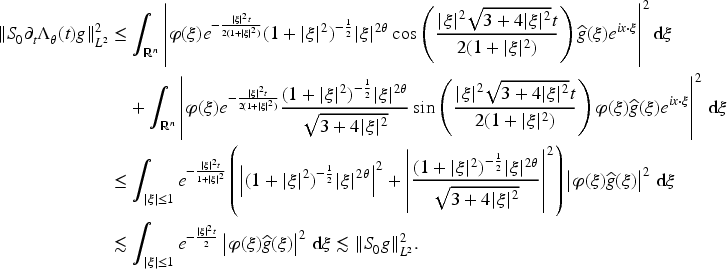
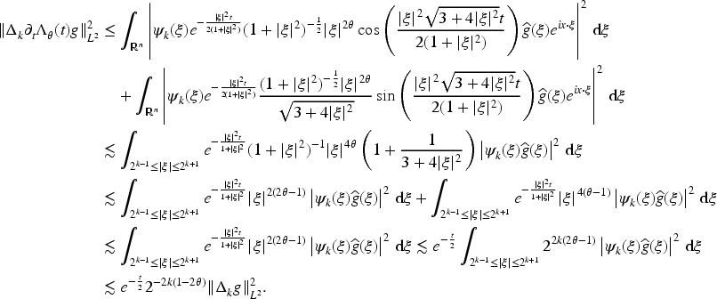
On the other hand,
$\begin{aligned} ‖ Δ_{k} \partial_{t}^{2} Λ_{θ} (t) g ‖_{L^{2}}^{2} & \leq \int_{R^{n}} {| ψ_{k} (ξ) e^{- \frac{| ξ |^{2} t}{2 (1 + | ξ |^{2})}} \frac{| ξ |^{2 (θ + 1)}}{(1 + | ξ |^{2})^{\frac{3}{2}}} \cos (\frac{| ξ |^{2} \sqrt{3 + 4 | ξ |^{2}} t}{2 (1 + | ξ |^{2})}) \hat{g} (ξ) e^{i x \cdot ξ} |}^{2} d ξ \\ + \int_{R^{n}} {| ψ_{k} (ξ) e^{- \frac{| ξ |^{2} t}{2 (1 + | ξ |^{2})}} \frac{| ξ |^{2 (θ + 1)} (1 + 2 | ξ |^{2})}{(1 + | ξ |^{2})^{\frac{3}{2}} \sqrt{3 + 4 | ξ |^{2}}} \sin (\frac{| ξ |^{2} \sqrt{3 + 4 | ξ |^{2}} t}{2 (1 + | ξ |^{2})}) \hat{g} (ξ) e^{i x \cdot ξ} |}^{2} d ξ \\ ≲ \int_{2^{k - 1} \leq | ξ | \leq 2^{k + 1}} e^{- \frac{| ξ |^{2} t}{1 + | ξ |^{2}}} \frac{| ξ |^{4 (θ + 1)}}{(1 + | ξ |^{2})^{3}} {| ψ_{k} (ξ) \hat{g} (ξ) |}^{2} d ξ \\ + \int_{2^{k - 1} \leq | ξ | \leq 2^{k + 1}} e^{- \frac{| ξ |^{2} t}{1 + | ξ |^{2}}} \frac{| ξ |^{4 (θ + 1)} (1 + 2 | ξ |^{2})^{2}}{(1 + | ξ |^{2})^{3} (3 + 4 | ξ |^{2})} {| ψ_{k} (ξ) \hat{g} (ξ) |}^{2} d ξ \\ ≲ e^{- \frac{t}{2}} \int_{2^{k - 1} \leq | ξ | \leq 2^{k + 1}} 2^{2 k (2 θ - 1)} {| ψ_{k} (ξ) \hat{g} (ξ) |}^{2} d ξ + e^{- \frac{t}{2}} \int_{2^{k - 1} \leq | ξ | \leq 2^{k + 1}} 2^{2 k (2 θ - 1)} {| ψ_{k} (ξ) \hat{g} (ξ) |}^{2} d ξ \\ ≲ \int_{2^{k - 1} \leq | ξ | \leq 2^{k + 1}} e^{- \frac{| ξ |^{2} t}{1 + | ξ |^{2}}} | ξ |^{2 (2 θ - 1)} {| ψ_{k} (ξ) \hat{g} (ξ) |}^{2} d ξ ≲ e^{- \frac{t}{2}} \int_{2^{k - 1} \leq | ξ | \leq 2^{k + 1}} 2^{k 4 v} {| ψ_{k} (ξ) \hat{g} (ξ) |}^{2} d ξ \\ ≲ e^{- \frac{t}{2}} 2^{k 4 θ} ‖ Δ_{k} g ‖_{L^{2}}^{2} . \end{aligned}$
Thus,
$‖ Δ_{k} \partial_{t}^{2} Λ_{θ} (t) g ‖_{L^{2}} ≲ e^{- \frac{t}{4}} 2^{k 2 θ} ‖ Δ_{k} g ‖_{L^{2}} .$
(3.46)
Taking into account that there exists $C = C_{n, θ} > 0$ such that $e^{- \frac{t}{4}} \leq C (1 + t)^{- \frac{n}{2} - (θ + 1)},$ from (3.39) and (3.45), multiplying by $2^{k (s - 1)}$ and taking the $l^{q} -$ norm, we obtain
$‖ \partial_{t}^{2} Λ_{θ} (t) g ‖_{B_{\infty, q}^{s - 1}} ≲ (1 + t)^{- \frac{n}{2} - (θ + 1)} ‖ g ‖_{B_{1, q}^{s - 1 + n + 2 θ}} .$
(3.47)
Similarly, since $e^{- \frac{t}{4}} \leq C (1 + t)^{- (θ + 1)}$ for some $C = C_{n, θ} > 0,$ from (3.42) and (3.46), multiplying by $2^{k (s - 1)}$ and taking the $l^{q} -$ norm, we get
$‖ \partial_{t} Λ_{θ} (t) g ‖_{B_{2, q}^{s - 1}} ≲ (1 + t)^{- (θ + 1)} ‖ g ‖_{B_{1, q}^{s - 1 + 2 θ}} .$
(3.48)
Finally, using complex interpolation, from (3.47) and (3.48) we arrive at (3.37).
3.2. Linear Estimates for Initial Data

Lemma 3.6
Assume that $2 \leq p \leq \infty$ and $1 \leq q \leq \infty$ with $\frac{1}{p} + \frac{1}{p^{'}} = 1$ and $s \in R$ . Then, there exists a constant $C = C_{n} > 0,$ depending only on $n,$ such that
$‖ \partial_{t} S (t) g ‖_{B_{p, q}^{s}} \leq C t^{- \frac{n}{2} (1 - \frac{2}{p})} ‖ g ‖_{B_{p^{'}, q}^{s + n (1 - \frac{2}{p})}},$
(3.49)
for all $g \in B_{p^{'}, q}^{s + n (1 - \frac{2}{p})} (R^{n})$ and $t > 0$ .
Proof.
Notice that $\partial_{t} S (t) g = \partial_{t} Λ_{0} (t) (I - Δ)^{\frac{1}{2}} g = (I - Δ)^{\frac{1}{2}} \partial_{t} Λ_{0} (t) g .$ Thus,
$‖ \partial_{t} S (t) g ‖_{B_{p, q}^{s}} = ‖ (I - Δ)^{\frac{1}{2}} \partial_{t} Λ_{0} (t) g ‖_{B_{p, q}^{s}} \leq ‖ \partial_{t} Λ_{0} (t) g ‖_{B_{p, q}^{s + 1}} .$
Then, applying Lemma 3.2 we conclude the proof.
Lemma 3.7
Assume that $2 \leq p \leq \infty$ and $1 \leq q \leq \infty$ with $\frac{1}{p} + \frac{1}{p^{'}} = 1$ and $s \in R$ . Then, there exists a constant $C = C_{n} > 0$ such that
$\begin{aligned} ‖ S (t) Δ g ‖_{B_{p, q}^{s}} & \leq C t^{- \frac{n}{2} (1 - \frac{2}{p})} ‖ g ‖_{B_{p^{'}, q}^{s + 1 + n (1 - \frac{2}{p})}}, \end{aligned}$

$\begin{aligned} ‖ \partial_{t} S (t) Δ g ‖_{B_{p, q}^{s - 1}} & \leq C t^{- \frac{n}{2} (1 - \frac{2}{p})} ‖ g ‖_{B_{p^{'}, q}^{s + 1 + n (1 - \frac{2}{p})}}, \end{aligned}$
for all $g \in B_{p^{'}, q}^{s + 1 + n (1 - \frac{2}{p})} (R^{n})$ and $t > 0$ .
Proof.
Notice that $S (t) Δ g = - Λ_{1} (t) (I - Δ)^{\frac{1}{2}} g,$ using Lemma 3.1 with $θ = 1,$ we obtain
$‖ S (t) Δ g ‖_{B_{p, q}^{s}} \leq C t^{- \frac{n}{2} (1 - \frac{2}{p})} {‖ (I - Δ)^{\frac{1}{2}} g ‖}_{B_{p^{'}, q}^{s + n (1 - \frac{2}{p})}} \leq C t^{- \frac{n}{2} (1 - \frac{2}{p})} ‖ g ‖_{B_{p^{'}, q}^{s + 1 + n (1 - \frac{2}{p})}} .$
In the last inequality we use that $(I - Δ)^{\frac{r}{2}} : B_{p, q}^{s} \to B_{p, q}^{s - r},$ for all $r \in R .$ This finishes the proof of the first inequality of the lemma. On the other hand, since $\partial_{t} S (t) Δ g = - \partial_{t} Λ_{1} (t) (I - Δ)^{\frac{1}{2}} g,$ using Lemma 3.2 with $θ = 1,$ we obtain
$‖ \partial_{t} S (t) Δ g ‖_{B_{p, q}^{s - 1}} \leq C t^{- \frac{n}{2} (1 - \frac{2}{p})} ‖ (I - Δ)^{\frac{1}{2}} g ‖_{B_{p^{'}, q}^{s + n (1 - \frac{2}{p})}} \leq C t^{- \frac{n}{2} (1 - \frac{2}{p})} ‖ g ‖_{B_{p^{'}, q}^{s + 1 + n (1 - \frac{2}{p})}},$
which finishes the proof of the lemma.
Lemma 3.8
Assume that $1 \leq q \leq \infty, 2 \leq p \leq \infty$ with $\frac{1}{p} + \frac{1}{p^{'}} = 1,$ and consider $s \in R .$ Then, there exists a constant $C = C_{n} > 0$ such that
$‖ \partial_{t}^{2} S (t) g ‖_{B_{p, q}^{s - 1}} \leq C t^{- \frac{n}{2} (1 - \frac{2}{p})} ‖ g ‖_{B_{p^{'}, q}^{s + n (1 - \frac{2}{p})}},$
for all $g \in B_{p^{'}, q}^{s + n (1 - \frac{2}{p})} (R^{n})$ and $t > 0$ .
Proof.
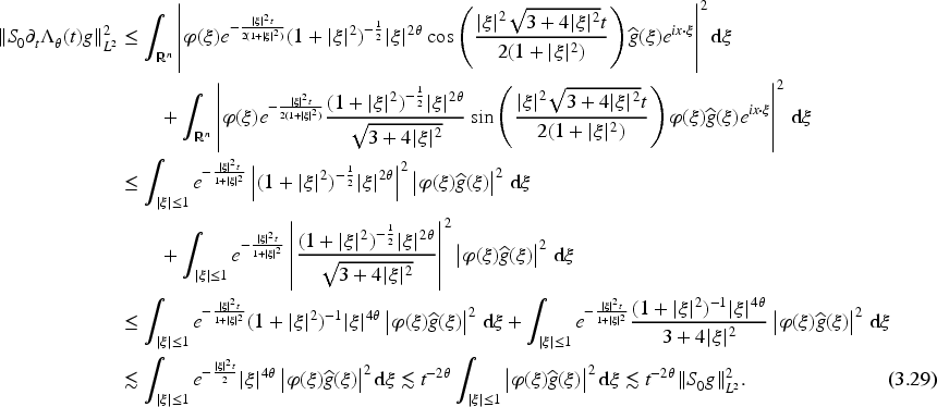
Observe that
$\begin{aligned} | S_{0} \partial_{t}^{2} S (t) g (x) | & \leq | \int_{R^{n}} φ (ξ) e^{- \frac{| ξ |^{2} t}{2 (1 + | ξ |^{2})}} \frac{| ξ |^{2}}{1 + | ξ |^{2}} \cos (\frac{| ξ |^{2} \sqrt{3 + 4 | ξ |^{2}} t}{2 (1 + | ξ |^{2})}) \hat{g} (ξ) e^{i x \cdot ξ} d ξ | \\ + | \int_{R^{n}} φ (ξ) e^{- \frac{| ξ |^{2} t}{2 (1 + | ξ |^{2})}} \frac{| ξ |^{2} (1 + 2 | ξ |^{2})}{(1 + | ξ |^{2}) \sqrt{3 + 4 | ξ |^{2}}} \sin (\frac{| ξ |^{2} \sqrt{3 + 4 | ξ |^{2}} t}{2 (1 + | ξ |^{2})}) \hat{g} (ξ) e^{i x \cdot ξ} d ξ | \\ ≲ ‖ φ (ξ) \hat{g} ‖_{L^{\infty}} \int_{| ξ | \leq 1} e^{- \frac{| ξ |^{2} t}{2 (1 + | ξ |^{2})}} d ξ ≲ ‖ S_{0} g ‖_{L^{1}} \int_{| ξ | \leq 1} e^{- \frac{| ξ |^{2} t}{4}} d ξ ≲ t^{- \frac{n}{2}} ‖ S_{0} g ‖_{L^{1}} . \end{aligned}$
Therefore,
$‖ S_{0} \partial_{t}^{2} S (t) g ‖_{L^{\infty}} ≲ t^{- \frac{n}{2}} ‖ S_{0} g ‖_{L^{1}} .$
(3.50)
On the other hand
$\begin{aligned} ‖ S_{0} \partial_{t}^{2} S (t) g ‖_{L^{2}}^{2} & \leq \int_{R^{n}} {| φ (ξ) e^{- \frac{| ξ |^{2} t}{2 (1 + | ξ |^{2})}} \frac{| ξ |^{2}}{1 + | ξ |^{2}} \cos (\frac{| ξ |^{2} \sqrt{3 + 4 | ξ |^{2}} t}{2 (1 + | ξ |^{2})}) \hat{g} (ξ) e^{i x \cdot ξ} |}^{2} d ξ \\ + \int_{R^{n}} {| φ (ξ) e^{- \frac{| ξ |^{2} t}{2 (1 + | ξ |^{2})}} \frac{| ξ |^{2} (1 + 2 | ξ |^{2})}{(1 + | ξ |^{2}) \sqrt{3 + 4 | ξ |^{2}}} \sin (\frac{| ξ |^{2} \sqrt{3 + 4 | ξ |^{2}} t}{2 (1 + | ξ |^{2})}) \hat{g} (ξ) e^{i x \cdot ξ} |}^{2} d ξ \\ ≲ \int_{| ξ | \leq 1} e^{- \frac{| ξ |^{2} t}{2}} {| φ (ξ) \hat{g} (ξ) |}^{2} d ξ ≲ ‖ S_{0} g ‖_{L^{2}}^{2} . \end{aligned}$
Thus we get
$‖ S_{0} \partial_{t}^{2} S (t) g ‖_{L^{2}} ≲ ‖ S_{0} g ‖_{L^{2}} .$
(3.51)
Now, consider $k \geq 1,$ then
$\begin{aligned} | Δ_{k} \partial_{t}^{2} S (t) g (x) | & \leq | \int_{R^{n}} ψ_{k} (ξ) e^{- \frac{| ξ |^{2} t}{2 (1 + | ξ |^{2})}} \frac{| ξ |^{2}}{1 + | ξ |^{2}} \cos (\frac{| ξ |^{2} \sqrt{3 + 4 | ξ |^{2}} t}{2 (1 + | ξ |^{2})}) \hat{g} (ξ) e^{i x \cdot ξ} d ξ | \\ + | \int_{R^{n}} ψ_{k} (ξ) e^{- \frac{| ξ |^{2} t}{2 (1 + | ξ |^{2})}} \frac{| ξ |^{2} (1 + 2 | ξ |^{2})}{(1 + | ξ |^{2}) \sqrt{3 + 4 | ξ |^{2}}} \sin (\frac{| ξ |^{2} \sqrt{3 + 4 | ξ |^{2}} t}{2 (1 + | ξ |^{2})}) \hat{g} (ξ) e^{i x \cdot ξ} d ξ | \\ ≲ ‖ ψ_{k} (ξ) \hat{g} ‖_{L^{\infty}} \int_{2^{k - 1} ≲ | ξ | \leq 2^{k + 1}} e^{- \frac{| ξ |^{2} t}{2 (1 + | ξ |^{2})}} \frac{| ξ |^{2} d ξ}{\sqrt{3 + 4 | ξ |^{2}}} \\ ≲ e^{- \frac{t}{4}} ‖ Δ_{k} g ‖_{L^{1}} \int_{2^{k - 1} \leq | ξ | \leq 2^{k + 1}} 2^{k} d ξ ≲ e^{- \frac{t}{4}} 2^{(n + 1) k} ‖ Δ_{k} g ‖_{L^{1}} . \end{aligned}$
Since $e^{- \frac{t}{4}} ≲ t^{- \frac{n}{2}},$ we obtain
${‖ Δ_{k} \partial_{t}^{2} S (t) g ‖}_{L^{\infty}} ≲ t^{- \frac{n}{2}} 2^{(n + 1) k} ‖ Δ_{k} g ‖_{L^{1}} .$
(3.52)
From (3.50) and (3.52), multiplying by $2^{k (s - 1)}$ and taking the $l^{q} -$ norm, we arrive at
${‖ \partial_{t}^{2} S (t) g ‖}_{B_{\infty, q}^{s - 1}} ≲ t^{- \frac{n}{2}} ‖ g ‖_{B_{1, q}^{s + n}} .$
(3.53)
For the estimate on $L^{2},$ we have
$\begin{aligned} ‖ Δ_{k} \partial_{t}^{2} S (t) g ‖_{L^{2}}^{2} & \leq \int_{R^{n}} {| ψ_{k} (ξ) e^{- \frac{| ξ |^{2} t}{2 (1 + | ξ |^{2})}} \frac{| ξ |^{2}}{1 + | ξ |^{2}} \cos (\frac{| ξ |^{2} \sqrt{3 + 4 | ξ |^{2}} t}{2 (1 + | ξ |^{2})}) \hat{g} (ξ) e^{i x \cdot ξ} |}^{2} d ξ \\ + \int_{R^{n}} {| ψ_{k} (ξ) e^{- \frac{| ξ |^{2} t}{2 (1 + | ξ |^{2})}} \frac{| ξ |^{2} (1 + 2 | ξ |^{2})}{(1 + | ξ |^{2}) \sqrt{3 + 4 | ξ |^{2}}} \sin (\frac{| ξ |^{2} \sqrt{3 + 4 | ξ |^{2}} t}{2 (1 + | ξ |^{2})}) \hat{g} (ξ) e^{i x \cdot ξ} |}^{2} d ξ \\ ≲ \int_{2^{k - 1} \leq | ξ | \leq 2^{k + 1}} 2^{2 k} {| ψ_{k} (ξ) \hat{g} (ξ) |}^{2} d ξ ≲ 2^{2 k} \int_{2^{k - 1} \leq | ξ | \leq 2^{k + 1}} {| ψ_{k} (ξ) \hat{g} (ξ) |}^{2} d ξ \\ ≲ 2^{2 k} ‖ Δ_{k} g ‖_{L^{2}}^{2} . \end{aligned}$
Then, we obtain
$‖ Δ_{k} \partial_{t}^{2} S (t) g ‖_{L^{2}} ≲ 2^{k} ‖ Δ_{k} g ‖_{L^{2}} .$
(3.54)
From (3.51) and (3.54), multiplying by $2^{k (s - 1)}$ and taking the $l^{q} -$ norm, we arrive at
$‖ \partial_{t}^{2} S (t) g ‖_{B_{2, q}^{s - 1}} ≲ ‖ g ‖_{B_{2, q}^{s}} .$
(3.55)
The desired result follows from (3.53), (3.55) and complex interpolation.
Lemma 3.9
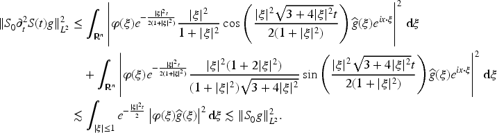
Let $s \in R,$ $2 \leq p \leq \infty$ and $1 \leq q \leq \infty$ . Then, there exists a constant $C = C_{p, n} > 0$ such that
$\begin{aligned} ‖ \partial_{t} S (t) g ‖_{B_{p, q}^{s}} & \leq C (1 + t)^{- \frac{n}{2} (1 - \frac{2}{p})} ‖ g ‖_{B_{p^{'}, q}^{s + n (1 - \frac{2}{p})}}, \end{aligned}$
(3.56)

$\begin{aligned} {‖ \partial_{t}^{2} S (t) g ‖}_{B_{p, q}^{s - 1}} & \leq C (1 + t)^{- \frac{n}{2} (1 - \frac{2}{p}) - 1} ‖ g ‖_{B_{p^{'}, q}^{s + n (1 - \frac{2}{p})}}, \end{aligned}$
(3.57)
for all $g \in B_{p^{'}, q}^{s + n (1 - \frac{2}{p})} (R^{n})$ and $t > 0$ .
Proof.
Notice that $\partial_{t} S (t) g = \partial_{t} Λ_{0} (t) (I - Δ)^{\frac{1}{2}} g = (I - Δ)^{\frac{1}{2}} \partial_{t} Λ_{0} (t) g .$ Thus,
$‖ \partial_{t} S (t) g ‖_{B_{p, q}^{s}} = ‖ (I - Δ)^{\frac{1}{2}} \partial_{t} Λ_{0} (t) g ‖_{B_{p, q}^{s}} \leq ‖ \partial_{t} Λ_{0} (t) g ‖_{B_{p, q}^{s + 1}} .$
In the last inequality we have used that $(I - Δ)^{\frac{r}{2}} : B_{p, q}^{s} \to B_{p, q}^{s - r},$ for all $r \in R .$ Thus, (3.49) follows from Lemma 3.2. On the other hand, it holds that $\partial_{t}^{2} S (t) g = \partial_{t}^{2} Λ_{0} (t) (I - Δ)^{\frac{1}{2}} g = (I - Δ)^{\frac{1}{2}} \partial_{t}^{2} Λ_{0} (t) g .$ Thus,
${‖ \partial_{t}^{2} S (t) g ‖}_{B_{p, q}^{s - 1}} = ‖ (I - Δ)^{\frac{1}{2}} \partial_{t}^{2} Λ_{0} (t) g ‖_{B_{p, q}^{s - 1} (R^{n})} \leq ‖ \partial_{t}^{2} Λ_{0} (t) g ‖_{B_{p, q}^{s}} .$
In the last inequality we have used that $(I - Δ)^{\frac{r}{2}} : B_{p, q}^{s} \to B_{p, q}^{s - r},$ for all $r \in R .$ Then, (3.57) follows from Lemma 3.5.
Lemma 3.10
Let $s \in R,$ $2 \leq p \leq \infty$ and $1 \leq q \leq \infty$ . Then, there exists $C = C_{p, n} > 0$ such that
$\begin{aligned} ‖ S (t) Δ g ‖_{B_{p, q}^{s}} & \leq C (1 + t)^{- \frac{n}{2} (1 - \frac{2}{p})} ‖ g ‖_{B_{p^{'}, q}^{s + 1 + n (1 - \frac{2}{p})}}, \\ ‖ \partial_{t} S (t) Δ g ‖_{B_{p, q}^{s - 1}} & \leq C (1 + t)^{- \frac{n}{2} (1 - \frac{2}{p}) - 1} ‖ g ‖_{B_{p^{'}, q}^{s + 1 + n (1 - \frac{2}{p})}}, \end{aligned}$
for all $g \in B_{p^{'}, q}^{s + 1 + n (1 - \frac{2}{p})} (R^{n})$ and $t > 0$ .
Proof.
Notice that $S (t) Δ g = - (I - Δ)^{\frac{1}{2}} Λ_{1} (t) g .$ Then, using Lemma 3.3 with $θ = 1,$ we obtain
$‖ S (t) Δ g ‖_{B_{p, q}^{s}} = ‖ (I - Δ)^{\frac{1}{2}} Λ_{1} (t) g ‖_{B_{p, q}^{s}} \leq C ‖ Λ_{1} (t) g ‖_{B_{p, q}^{s + 1}} \leq C (1 + t)^{- \frac{n}{2} (1 - \frac{2}{p})} ‖ g ‖_{B_{p^{'}, q}^{s + 1 + n (1 - \frac{2}{p})}} .$
On the other hand, notice that $\partial_{t} S (t) Δ g = - (I - Δ)^{\frac{1}{2}} \partial_{t} Λ_{1} (t) g$ . From Lemma 3.4 with $θ = 1,$ we get
$‖ \partial_{t} S (t) Δ g ‖_{B_{p, q}^{s - 1}} = ‖ (I - Δ)^{\frac{1}{2}} \partial_{t} Λ_{1} (t) g ‖_{B_{p, q}^{s - 1}} \leq C ‖ \partial_{t} Λ_{1} (t) g ‖_{B_{p, q}^{s}} \leq C (1 + t)^{- \frac{n}{2} (1 - \frac{2}{p}) - 1} ‖ g ‖_{B_{p^{'}, q}^{s + 1 + n (1 - \frac{2}{p})}} .$

3.3. Product Estimates

In this subsection we derive a product estimate which is key in the proof of existence results. Its proof follows the ideas of the product estimate in Ferreira and Pérez-López (2020).

Lemma 3.11 (Product estimate)

Let $λ, p$ such that $λ p^{'} > p$ and assume that given $s$ the conditions (H1)–(H5) are verified. Then,

{‖ \prod_{i = 1}^{λ} u_{i} ‖}_{B_{p^{'}, \infty}^{λ (s - (\frac{n}{p} - \frac{n}{λ p^{'}}))}} \leq C \prod_{i = 1}^{λ} {‖ u_{i} ‖}_{B_{p, \infty}^{s}},

(3.58)

for all

u_{i} \in B_{p, \infty}^{s} (R^{n}),

i = 1, 2, \dots, λ .

Remark 3.12

Even the product estimate proved in Wang et al. (2011), Lemma 4.1, includes some cases for $λ$ no integer, it imposes among its conditions, that $s \geq \frac{n}{p} - \frac{n}{λ p^{'}},$ which rules out some cases included in our estimate (3.58); for instance, considering $λ = 2$ , $p = 2$ , $p^{'} = 2$ and $p_{2} = \frac{4}{3}$ , the inequality (3.58) is true for $s$ verifying

\frac{n}{8} = \frac{n}{p} - \frac{n}{λ p_{2}} < s < 2 (\frac{n}{p} - \frac{n}{λ p_{2}}) = \frac{n}{4} = \frac{n}{p} - \frac{n}{λ p^{'}} .

4. Existence of Solutions and Asymptotic Stability

4.1. Existence of Local Solutions. Proof of Theorem 2.2

For convenience in the written, we denote by

\begin{aligned} {‖ u ‖}_{X_{p, \infty, T}^{s, α}} & := sup_{0 \leq t \leq T} t^{α} ‖ u (t) ‖_{B_{p, \infty}^{s}}, {‖ v ‖}_{Y_{p, \infty, T}^{s - 1, α}} := sup_{0 \leq t \leq T} t^{α} ‖ v (t) ‖_{B_{p, \infty}^{s - 1}} \end{aligned}

\begin{aligned} {‖ [u, u_{t}] ‖}_{Z_{T}^{s}} & := {‖ u ‖}_{X_{p, \infty, T}^{s, α}} + {‖ u_{t} ‖}_{Y_{p, \infty, T}^{s - 1, α}} . \end{aligned}

Proposition 4.1
Let $α = \frac{n}{2} (1 - \frac{2}{p})$ , $θ \in [0, 1]$ , and $λ, p, s$ as in Lemma 3.11. In addition, assume that $s + n (1 - \frac{2}{p}) - 2 (1 - θ) \leq λ (s - (\frac{n}{p} - \frac{n}{λ p^{'}})),$ and $0 \leq α < \frac{1}{λ}$ . Then
${‖ \int_{0}^{t} S (t - τ) (I - Δ)^{- 1} (- Δ)^{θ} [u^{λ} (τ) - v^{λ} (τ)] d τ ‖}_{X_{p, \infty, T}^{s, α}} \leq C T^{2 - θ - α λ} ‖ u - v ‖_{X_{p, \infty, T}^{s, α}} \sum_{i = 0}^{λ - 1} ‖ u ‖_{X_{p, q, T}^{s, α}}^{(λ - 1) - i} ‖ v ‖_{X_{p, \infty, T}^{s, α}}^{i} .$

Proof.
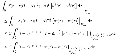
Notice that $S (t - τ) (I - Δ)^{- 1} (- Δ)^{θ} f = Λ_{θ} (t - τ) (I - Δ)^{- \frac{1}{2}} f$ . Then, by Lemma 3.1 we obtain
$\begin{aligned} {‖ \int_{0}^{t} S (t - τ) (I - Δ)^{- 1} (- Δ)^{θ} [u^{λ} (τ) - v^{λ} (τ)] d τ ‖}_{B_{p, \infty}^{s}} \\ \leq \int_{0}^{t} {‖ Λ_{θ} (t - τ) (I - Δ)^{- \frac{1}{2}} [u^{λ} (τ) - v^{λ} (τ)] ‖}_{B_{p, \infty}^{s}} d τ \\ \leq C \int_{0}^{t} (t - τ)^{- α + 1 - θ} ‖ (I - Δ)^{- \frac{1}{2}} [u^{λ} (τ) - v^{λ} (τ)] ‖_{B_{p^{'}, \infty}^{s + n (1 - \frac{2}{p}) - (1 - 2 θ)}} d τ \\ \leq C \int_{0}^{t} (t - τ)^{- α + 1 - θ} ‖ u^{λ} (τ) - v^{λ} (τ) ‖_{B_{p^{'}, \infty}^{s + n (1 - \frac{2}{p}) - 2 (1 - θ)}} d τ . \end{aligned}$
Since $s + n (1 - \frac{2}{p}) - 2 (1 - θ) \leq λ (s - (\frac{n}{p} - \frac{n}{λ p^{'}})),$ we arrive at
$\begin{aligned} {‖ \int_{0}^{t} S (t - τ) (I - Δ)^{- 1} (- Δ)^{θ} [u^{λ} (τ) - v^{λ} (τ)] d τ ‖}_{B_{p, \infty}^{s}} \\ \leq C \int_{0}^{t} (t - τ)^{- α + 1 - θ} ‖ u^{λ} (τ) - v^{λ} (τ) ‖_{B_{p^{'}, \infty}^{λ (s - (\frac{n}{p} - \frac{n}{λ p^{'}}))}} d τ \\ = C \int_{0}^{t} (t - τ)^{- α + 1 - θ} ‖ [u (τ) - v (τ)] \sum_{i = 0}^{λ - 1} u^{(λ - 1) - i} (τ) v^{i} (τ) ‖_{B_{p^{'}, \infty}^{λ (s - (\frac{n}{p} - \frac{n}{λ p^{'}}))}} d τ \\ \leq C \int_{0}^{t} (t - τ)^{- α + 1 - θ} ‖ u (τ) - v (τ) ‖_{B_{p, q}^{s}} \sum_{i = 0}^{λ - 1} ‖ u (τ) ‖_{B_{p, \infty}^{s}}^{(λ - 1) - i} ‖ v (τ) ‖_{B_{p, q}^{s}}^{i} d τ \\ \leq C ‖ u - v ‖_{X_{p, \infty, T}^{s, α}} \sum_{i = 0}^{λ - 1} ‖ u ‖_{X_{p, \infty, T}^{s, α}}^{(λ - 1) - i} ‖ v ‖_{X_{p, \infty, T}^{s, α}}^{i} \int_{0}^{t} (t - τ)^{- α + 1 - θ} τ^{- α λ} d τ \\ \leq C ‖ u - v ‖_{X_{p, \infty, T}^{s, α}} \sum_{i = 0}^{λ - 1} ‖ u ‖_{X_{p, \infty, T}^{s, α}}^{(λ - 1) - i} ‖ v ‖_{X_{p, \infty, T}^{s, α}}^{i} t^{2 - α - θ - α λ} . \end{aligned}$
Multiplying the last inequality by $t^{α}$ and taking the supremum on $t,$ we arrive at the desired result.
Lemma 4.2
Let $α = \frac{n}{2} (1 - \frac{2}{p})$ , $θ \in [0, 1]$ , and $λ, p, s$ as in Lemma 3.11. In addition, assume that $s + n (1 - \frac{2}{p}) - 2 (1 - θ) \leq λ (s - (\frac{n}{p} - \frac{n}{λ p^{'}}))$ and $0 \leq α < \frac{1}{λ}$ . Then
${‖ \int_{0}^{t} \partial_{t} S (t - τ) (I - Δ)^{- 1} (- Δ)^{θ} [u^{λ} (τ) - v^{λ} (τ)] d τ ‖}_{Y_{p, \infty, T}^{s, α}} \leq C T^{1 - α λ} ‖ u - v ‖_{X_{p, q, T}^{s, α}} \sum_{i = 0}^{λ - 1} ‖ u ‖_{X_{p, \infty, T}^{s, α}}^{(λ - 1) - i} ‖ v ‖_{X_{p, \infty, T}^{s, α}}^{i} .$

Proof.
Observe that $\partial_{t} S (t - τ) (I - Δ)^{- 1} (- Δ)^{θ} f = \partial_{t} Λ_{θ} (t - τ) (I - Δ)^{- \frac{1}{2}} f$ . Then, by Lemma 3.2 we obtain
$\begin{aligned} {‖ \int_{0}^{t} \partial_{t} S (t - τ) (I - Δ)^{- 1} (- Δ)^{θ} [u^{λ} (τ) - v^{λ} (τ)] d τ ‖}_{B_{p, \infty}^{s - 1}} \\ \leq \int_{0}^{t} {‖ \partial_{t} Λ_{θ} (t - τ) (I - Δ)^{- \frac{1}{2}} [u^{λ} (τ) - v^{λ} (τ)] ‖}_{B_{p, \infty}^{s - 1}} d τ \\ \leq C \int_{0}^{t} (t - τ)^{- α} {‖ (I - Δ)^{- \frac{1}{2}} [u^{λ} (τ) - v^{λ} (τ)] ‖}_{B_{p^{'}, \infty}^{s + n (1 - \frac{2}{p}) - (1 - 2 θ)}} d τ . \end{aligned}$
Since $(I - Δ)^{- \frac{1}{2}} : B_{p, \infty}^{r - 1} \to B_{p, \infty}^{r},$ from Lemma 3.11 and the last inequality, we arrive at
$\begin{aligned} {‖ \int_{0}^{t} \partial_{t} S (t - τ) (I - Δ)^{- 1} (- Δ)^{θ} [u^{λ} (τ) - v^{λ} (τ)] d τ ‖}_{B_{p, \infty}^{s - 1}} \\ \leq C \int_{0}^{t} (t - τ)^{- α} ‖ u^{λ} (τ) - v^{λ} (τ) ‖_{B_{p^{'}, \infty}^{s + n (1 - \frac{2}{p}) - 2 (1 - θ)}} d τ \\ \leq C \int_{0}^{t} (t - τ)^{- α} ‖ u^{λ} (τ) - v^{λ} (τ) ‖_{B_{p^{'}, \infty}^{λ (s - (\frac{n}{p} - \frac{n}{λ p^{'}}))}} d τ \\ \leq C ‖ u - v ‖_{X_{p, \infty, T}^{s, α}} \sum_{i = 0}^{λ - 1} ‖ u ‖_{X_{p, \infty, T}^{s, α}}^{(λ - 1) - i} ‖ v ‖_{X_{p, \infty, T}^{s, α}}^{i} \int_{0}^{t} (t - τ)^{- α} τ^{- α λ} d τ \\ \leq C ‖ u - v ‖_{X_{p, \infty, T}^{s, α}} \sum_{i = 0}^{λ - 1} ‖ u ‖_{X_{p, \infty, T}^{s, α}}^{(λ - 1) - i} ‖ v ‖_{X_{p, \infty, T}^{s, α}}^{i} t^{1 - α - α λ} . \end{aligned}$
Multiplying the last inequality by $t^{α}$ and taking the supremum on $t,$ we arrive at the desired result.

Consider the space of initial data $Z_{0}^{s}$ with norm
$‖ [u_{0}, u_{1}] ‖_{Z_{0}^{s}} = ‖ u_{0} ‖_{B_{p^{'}, \infty}^{s + n (1 - \frac{2}{p})}} + ‖ u_{1} ‖_{B_{p^{'}, \infty}^{s + 1 + n (1 - \frac{2}{p})}} .$

The proof of Theorem 2.2 is based on the Banach Fixed Point Theorem. For that, we consider the fixed point mapping $Ψ : Z_{T}^{s} \to Z_{T}^{s}$ defined by $Ψ ([u, u_{t}]) = [Ψ_{0} (u), Ψ_{1} (u_{t})],$ where
$\begin{aligned} Ψ_{0} (u) & := \partial_{t} S (t) u_{0} (x) + S (t) Δ u_{1} (x) - \int_{0}^{t} S (t - τ) (I - Δ)^{- 1} (- Δ)^{θ} [u (x, τ)]^{λ} d τ, \end{aligned}$

$\begin{aligned} Ψ_{1} (u_{t}) & := \partial_{t}^{2} S (t) u_{0} (x) + \partial_{t} S (t) Δ u_{1} (x) - \int_{0}^{t} \partial_{t} S (t - τ) (I - Δ)^{- 1} (- Δ)^{θ} [u (x, τ)]^{λ} d τ . \end{aligned}$

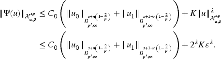
Consider $R = C ‖ [u_{0}, u_{1}] ‖_{Z_{0}^{s}},$ where $C$ is the maximum of the constants appearing in Lemmas 3.6, 3.7 and 3.8. We will show that $Ψ : \bar{B} (0, 2 R) \to \bar{B} (0, 2 R)$ is well-defined and is a contraction. Since we are interested in a local result, we assume that $T ≲ 1.$ Therefore $T^{2 - θ - α λ} ≲ T^{1 - α λ} .$ Now, from Lemmas 3.6, 3.7, 3.8, 4.1 and 4.2 (making $v = 0$ ), we obtain
$‖ Ψ ([u, u_{t}]) ‖_{Z_{T}^{s}} \leq C ‖ u_{0} ‖_{B_{p^{'}, \infty}^{s + n (1 - \frac{2}{p})}} + C ‖ u_{1} ‖_{B_{p^{'}, \infty}^{s + 1 + n (1 - \frac{2}{p})}} + K T^{1 - α λ} ‖ u ‖_{X_{p, \infty, T}^{s, α}}^{λ} \leq R + K T^{1 - α λ} (2 R)^{λ} .$

Now, chose $T > 0$ such that
$0 < T < \frac{1}{(2^{λ} λ R^{λ - 1} K)^{\frac{1}{1 - α λ}}} \leq \frac{1}{(2^{λ} R^{λ - 1} K)^{\frac{1}{1 - α λ}}} .$

Then, we arrive at
$‖ Ψ ([u, u_{t}]) ‖_{Z_{T}^{s}} \leq 2 R .$

On the other hand,
$\begin{aligned} ‖ Ψ ([u, u_{t}]) - Ψ ([\tilde{u}, {\tilde{u}}_{t}]) ‖_{Z_{T}^{s}} & = {‖ \int_{0}^{t} S (t - τ) (I - Δ)^{- 1} (- Δ)^{θ} (u^{λ} - {\tilde{u}}^{λ}) d τ ‖}_{X_{p, \infty, T}^{s, α}} \\ + {‖ \int_{0}^{t} \partial_{t} S (t - τ) (I - Δ)^{- 1} (- Δ)^{θ} (u^{λ} - {\tilde{u}}^{λ}) d τ ‖}_{Y_{p, \infty, T}^{s - 1, α}} \\ \leq K T^{1 - α λ} ‖ u - \tilde{u} ‖_{X_{p, \infty, T}^{s, α}} \sum_{i = 0}^{λ - 1} ‖ u ‖_{X_{p, \infty, T}^{s, α}}^{(λ - 1) - i} ‖ \tilde{u} ‖_{X_{p, \infty, T}^{s, α}}^{i} \\ \leq λ 2^{λ - 1} R^{λ - 1} K T^{1 - α λ} ‖ [u, u_{t}] - [\tilde{u}, {\tilde{u}}_{t}] ‖_{Z_{T}^{s}}, \end{aligned}$
and taking into account that
$λ 2^{λ - 1} R^{λ - 1} K T^{1 - α λ} < 1,$
we get that $Ψ$ is a contraction. Thus, the Banach Fixed Point Theorem implies that $Ψ$ has a unique fixed point in $Z_{T}^{s}$ which is a local solution of (2.2).
4.2. Existence of Global Solutions. Proof of Theorem 2.3.

For simplicity in writing, we use the following notation

{‖ u ‖}_{X_{α, β}^{s, p}} := sup_{t > 0} (1 + t)^{α} ‖ u ‖_{B_{p, \infty}^{s}} + sup_{t > 0} (1 + t)^{β} ‖ u_{t} ‖_{B_{p, \infty}^{s - 1}} .

Lemma 4.3
Let $α = \frac{n}{2} (1 - \frac{2}{p}) - (1 - θ)$ , $θ \in (\frac{2 - n}{2}, 1]$ and $λ, p, s$ as in Lemma 3.11. Moreover, assume that $s - 1 + n (1 - \frac{2}{p}) - 2 (1 - θ) \leq λ (s - (\frac{n}{p} - \frac{n}{λ p^{'}}))$ and $α > \frac{1}{λ}$ . Then,
$sup_{t > 0} (1 + t)^{α} {‖ \int_{0}^{t} S (t - τ) (I - Δ)^{- 1} (- Δ)^{θ} (u^{λ} - v^{λ}) d τ ‖}_{B_{p, \infty}^{s}} \leq C ‖ u - v ‖_{X_{α, β}^{s, p}} \sum_{i = 0}^{λ - 1} ‖ u ‖_{X_{α, β}^{s, p}}^{(λ - 1) - i} ‖ v ‖_{X_{α, β}^{s, p}}^{i} .$

Proof.
Notice that $S (t - τ) (I - Δ)^{- 1} (- Δ)^{θ} f = Λ_{θ} (t - τ) (I - Δ)^{- \frac{1}{2}} f$ . Thus, from Lemma 3.3 and since $‖ (I - Δ)^{- \frac{1}{2}} g ‖_{B_{p^{'}, \infty}^{r}} \leq C ‖ g |_{B_{p^{'}, \infty}^{r - 1}},$ we have
$\begin{aligned} {‖ \int_{0}^{t} S (t - τ) (I - Δ)^{- 1} (- Δ)^{θ} (u^{λ} - v^{λ}) d τ ‖}_{B_{p, \infty}^{s}} \\ \leq \int_{0}^{t} ‖ Λ_{θ} (t - τ) (I - Δ)^{- \frac{1}{2}} (u^{λ} - v^{λ}) ‖_{B_{p, \infty}^{s}} d τ \\ \leq C \int_{0}^{t} (1 + t - τ)^{- α} ‖ (I - Δ)^{- \frac{1}{2}} (u^{λ} - v^{λ}) ‖_{B_{p^{'}, \infty}^{s + n (1 - \frac{2}{p}) - 2 (1 - θ)}} d τ \\ \leq C \int_{0}^{t} (1 + t - τ)^{- α} ‖ u^{λ} - v^{λ} ‖_{B_{p^{'}, \infty}^{s - 1 + n (1 - \frac{2}{p}) - 2 (1 - θ)}} d τ \\ \leq C \int_{0}^{t} (1 + t - τ)^{- α} ‖ u^{λ} - v^{λ} ‖_{B_{p^{'}, \infty}^{γ (s - (\frac{n}{p} - \frac{n}{λ p^{'}}))}} d τ . \end{aligned}$
Using Lemma 3.11 and the last inequality, we obtain
$\begin{aligned} {‖ \int_{0}^{t} S (t - τ) (I - Δ)^{- 1} (- Δ)^{θ} (u^{λ} - v^{λ}) d τ ‖}_{B_{p, \infty}^{s}} \\ = C \int_{0}^{t} (1 + t - τ)^{- α} ‖ [u - v] \sum_{i = 0}^{λ - 1} u^{(λ - 1) - i} v^{i} (τ) ‖_{B_{p^{'}, \infty}^{λ (s - (\frac{n}{p} - \frac{n}{λ p^{'}}))}} d τ \\ \leq C \int_{0}^{t} (1 + t - τ)^{- α} ‖ u - v ‖_{B_{p, \infty}^{s}} \sum_{i = 0}^{λ - 1} ‖ u ‖_{B_{p, \infty}^{s}}^{(λ - 1) - i} ‖ v ‖_{B_{p, \infty}^{s}}^{i} d τ \\ \leq C ‖ u - v ‖_{X_{α, β}^{s, p}} \sum_{i = 0}^{λ - 1} ‖ u ‖_{X_{α, β}^{s, p}}^{(λ - 1) - i} ‖ v ‖_{X_{α, β}^{s, p}}^{i} \int_{0}^{t} (1 + t - τ)^{- α} (1 + τ)^{- α λ} d τ \\ \leq C ‖ u - v ‖_{X_{α, β}^{s, p}} \sum_{i = 0}^{λ - 1} ‖ u ‖_{X_{α, β}^{s, p}}^{(λ - 1) - i} ‖ v ‖_{X_{α, β}^{s, p}}^{i} (1 + t)^{- α} \int_{0}^{t} (1 + τ)^{- α λ} d τ \\ \leq C ‖ u - v ‖_{X_{α, β}^{s, p}} \sum_{i = 0}^{λ - 1} ‖ u ‖_{X_{α, β}^{s, p}}^{(λ - 1) - i} ‖ v ‖_{X_{α, β}^{s, p}}^{i} (1 + t)^{- α}, \end{aligned}$
which implies the desired result.
Lemma 4.4
Let $α = \frac{n}{2} (1 - \frac{2}{p}) - (1 - θ)$ , $β = \frac{n}{2} (1 - \frac{2}{p}) + θ$ , $θ \in (\frac{2 - n}{2}, 1]$ , and $λ, p, s$ as in Lemma 3.11. Moreover, assume that $s - 1 + n (1 - \frac{2}{p}) - 2 (1 - θ) \leq λ (s - (\frac{n}{p} - \frac{n}{λ p^{'}}))$ , $α > \frac{1}{λ}$ and $λ α \geq β$ . Then
$sup_{t > 0} (1 + t)^{β} {‖ \int_{0}^{t} \partial_{t} S (t - τ) (I - Δ)^{- 1} (- Δ)^{θ} (u^{λ} - v^{λ}) d τ ‖}_{B_{p, \infty}^{s - 1}} \leq C ‖ u - v ‖_{X_{α, β}^{s, p}} \sum_{i = 0}^{λ - 1} ‖ u ‖_{X_{α, β}^{s, p}}^{(λ - 1) - i} ‖ v ‖_{X_{α, β}^{s, p}}^{i} .$

Proof.
Notice that $\partial_{t} S (t - τ) (I - Δ)^{- 1} (- Δ)^{θ} f = \partial_{t} Λ_{θ} (t - τ) (I - Δ)^{- \frac{1}{2}} f$ . Thus, using Lemma 3.4 we have
$\begin{aligned} {‖ \int_{0}^{t} \partial_{t} S (t - τ) (I - Δ)^{- 1} (- Δ)^{θ} (u^{λ} - v^{λ}) d τ ‖}_{B_{p, \infty}^{s - 1}} \\ \leq \int_{0}^{t} ‖ \partial_{t} Λ_{θ} (t - τ) (I - Δ)^{- \frac{1}{2}} (u^{λ} - v^{λ}) ‖_{B_{p, \infty}^{s - 1}} d τ \\ \leq C \int_{0}^{t} (1 + t - τ)^{- β} ‖ (I - Δ)^{- \frac{1}{2}} (u^{λ} - v^{λ}) ‖_{B_{p^{'}, \infty}^{s + n (1 - \frac{2}{p}) - 2 (1 - θ)}} d τ \\ \leq C \int_{0}^{t} (1 + t - τ)^{- β} ‖ u^{λ} - v^{λ} ‖_{B_{p^{'}, \infty}^{s - 1 + n (1 - \frac{2}{p}) - 2 (1 - θ)}} d τ \\ \leq C \int_{0}^{t} (1 + t - τ)^{- β} ‖ u^{λ} - v^{λ} ‖_{B_{p^{'}, \infty}^{λ (s - (\frac{n}{p} - \frac{n}{λ p^{'}}))}} d τ . \end{aligned}$
From Lemma 3.11 and the last inequality, we arrive at
$\begin{aligned} {‖ \int_{0}^{t} \partial_{t} S (t - τ) (I - Δ)^{- 1} (- Δ)^{θ} (u^{λ} - v^{λ}) d τ ‖}_{B_{p, \infty}^{s - 1}} \\ \leq C \int_{0}^{t} (1 + t - τ)^{- β} ‖ [u - v] \sum_{i = 0}^{λ - 1} u^{(λ - 1) - i} v^{i} (τ) ‖_{B_{p^{'}, \infty}^{λ (s - (\frac{n}{p} - \frac{n}{λ p^{'}}))}} d τ \\ \leq C \int_{0}^{t} (1 + t - τ)^{- β} ‖ u - v ‖_{B_{p, \infty}^{s}} \sum_{i = 0}^{λ - 1} ‖ u ‖_{B_{p, q}^{s}}^{(λ - 1) - i} ‖ v ‖_{B_{p, \infty}^{s}}^{i} d τ \\ \leq C ‖ u - v ‖_{X_{α, β}^{s, p}} \sum_{i = 0}^{λ - 1} ‖ u ‖_{X_{α, β}^{s, p}}^{(λ - 1) - i} ‖ v ‖_{X_{α, β}^{s, p}}^{i} \int_{0}^{t} (1 + t - τ)^{- β} (1 + τ)^{- α λ} d τ \\ \leq C ‖ u - v ‖_{X_{α, β}^{s, p}} \sum_{i = 0}^{γ - 1} ‖ u ‖_{X_{α, β}^{s, p}}^{(λ - 1) - i} ‖ v ‖_{X_{α, β}^{s, p}}^{i} (1 + t)^{- β} \int_{0}^{t} (1 + τ)^{- α λ} d τ \\ \leq C ‖ u - v ‖_{X_{α, β}^{s, p}} \sum_{i = 0}^{γ - 1} ‖ u ‖_{X_{α, β}^{s, p}}^{(λ - 1) - i} ‖ v ‖_{X_{α, β}^{s, p}}^{i} (1 + t)^{- β}, \end{aligned}$
which implies the desired result. Now we are in position to use the Banach Fixed Point Theorem. For that, we consider the mapping
$Ψ (u) := \partial_{t} S (t) u_{0} (x) + S (t) Δ u_{1} (x) - \int_{0}^{t} S (t - τ) (I - Δ)^{- 1} (- Δ)^{θ} [u (x, τ)]^{λ} d τ .$
For $ε > 0$ suitable, we will prove that $Ψ : \bar{B} (0, 2 ε) \to \bar{B} (0, 2 ε)$ is well-defined and has a unique fixed point. Here, $\bar{B} (0, 2 ε) \subset X_{α, β}^{s, p}$ denotes the closed ball centered in $0$ and radius $2 ε$ . From Lemmas 3.9, 3.10, 4.3 and 4.4, it holds
$\begin{aligned} sup_{t > 0} (1 + t)^{α} ‖ Ψ (u) ‖_{B_{p, \infty}^{s}} \leq sup_{t > 0} (1 + t)^{α} ‖ \partial_{t} S (t) u_{0} ‖_{B_{p, \infty}^{s}} + sup_{t > 0} (1 + t)^{α} ‖ S (t) Δ u_{1} ‖_{B_{p, \infty}^{s}} \\ + sup_{t > 0} (1 + t)^{α} ‖ \int_{0}^{t} S (t - τ) (I - Δ)^{- 1} (- Δ)^{θ} u^{λ} d τ ‖_{B_{p, \infty}^{s}} \\ \leq C (sup_{t > 0} (1 + t)^{- (1 - θ)} ‖ u_{0} ‖_{B_{p^{'}, \infty}^{s + n (1 - \frac{2}{p})}} + sup_{t > 0} (1 + t)^{- (1 - θ)} ‖ u_{1} ‖_{B_{p^{'}, \infty}^{s + 1 + n (1 - \frac{2}{p})}} + ‖ u ‖_{X_{α, β}^{s, p}}^{λ}) \\ \leq C (‖ u_{0} ‖_{B_{p^{'}, \infty}^{s + n (1 - \frac{2}{p})}} + ‖ u_{1} ‖_{B_{p^{'}, \infty}^{s + 1 + n (1 - \frac{2}{p})}} + ‖ u ‖_{X_{α, β}^{s, p}}^{λ}) . \end{aligned}$
(4.1)
Moreover,
$\begin{aligned} sup_{t > 0} (1 + t)^{β} ‖ \partial_{t} Ψ (u) ‖_{B_{p, \infty}^{s - 1}} \leq sup_{t > 0} (1 + t)^{β} ‖ \partial_{t}^{2} S (t) u_{0} ‖_{B_{p, \infty}^{s - 1}} + sup_{t > 0} (1 + t)^{β} ‖ \partial_{t} S (t) Δ u_{1} (x) ‖_{B_{p, \infty}^{s - 1}} \\ + sup_{t > 0} (1 + t)^{β} ‖ \int_{0}^{t} \partial_{t} S (t - τ) (I - Δ)^{- 1} (- Δ)^{θ} [u (x, τ)]^{λ} d τ ‖_{B_{p, \infty}^{s - 1}} \\ \leq C (sup_{t > 0} (1 + t)^{- (1 - θ)} ‖ u_{0} ‖_{B_{p^{'}, \infty}^{s + n (1 - \frac{2}{p})}} + sup_{t > 0} (1 + t)^{- (1 - θ}) ‖ u_{1} ‖_{B_{p^{'}, \infty}^{s + 1 + n (1 - \frac{2}{p})}} + ‖ u ‖_{X_{α, β}^{s, p}}^{λ}) \\ \leq C (‖ u_{0} ‖_{B_{p^{'}, \infty}^{s + n (1 - \frac{2}{p})}} + ‖ u_{1} ‖_{B_{p^{'}, \infty}^{s + 1 + n (1 - \frac{2}{p})}} + ‖ u ‖_{X_{α, β}^{s, p}}^{λ}) \end{aligned}$
(4.2)
From (4.1) and (4.2) we arrive at
$\begin{aligned} ‖ Ψ (u) ‖_{X_{α, β}^{s, p}} & \leq C_{0} (‖ u_{0} ‖_{B_{p^{'}, \infty}^{s + n (1 - \frac{2}{p})}} + ‖ u_{1} ‖_{B_{p^{'}, \infty}^{s + 1 + n (1 - \frac{2}{p})}}) + K ‖ u ‖_{X_{α, β}^{s, p}}^{λ} \\ \leq C_{0} (‖ u_{0} ‖_{B_{p^{'}, \infty}^{s + n (1 - \frac{2}{p})}} + ‖ u_{1} ‖_{B_{p^{'}, \infty}^{s + 1 + n (1 - \frac{2}{p})}}) + 2^{λ} K ε^{λ} . \end{aligned}$
Choosing $ε > o$ such that
$0 < ε < {(\frac{1}{λ 2^{(λ - 1)} K})}^{1 / (λ - 1)} \leq {(\frac{1}{2^{λ} K})}^{1 / (λ - 1)},$
and $δ = \frac{ε}{C_{0}}$ we get
$‖ Ψ (u) ‖_{X_{α, β}^{s, p}} \leq 2 ε .$

On the other hand, from Lemmas 4.3 and 4.4, we get
$\begin{aligned} ‖ Ψ (u) - Ψ (v) ‖_{X_{α, β}^{s, p}} & = ‖ \int_{0}^{t} S (t - τ) (I - Δ)^{- 1} (- Δ)^{θ} (u^{λ} - v^{λ}) d τ ‖_{X_{α, β}^{s, p}} \\ \leq K ‖ u - v ‖_{X_{α, β}^{s, p}} \sum_{i = 0}^{λ - 1} ‖ u ‖_{X_{α, β}^{s, p}}^{(λ - 1) - i} ‖ v ‖_{X_{α, β}^{s, p}}^{i} \leq λ 2^{(λ - 1)} ε^{(λ - 1)} K ‖ u - v ‖_{X_{α, β}^{s, p}}, \end{aligned}$
and since that
$λ 2^{(λ - 1)} ε^{(p - 1)} K < 1,$
it follows that $Ψ$ is a contraction. Thus, by the Banach Fixed Point Theorem, we conclude that $Ψ$ has a unique fixed point which is the global solution of (2.2).
4.3. Asymptotic Stability. Proof of Theorem 2.4

In this subsection we prove Theorem 2.4. Let $u, \tilde{u},$ be two solutions of (2.2) with initial data $[u_{0}, u_{1}],$ $[{\tilde{u}}_{0}, {\tilde{v}}_{1}] \in B_{p^{'}, \infty}^{s + n (1 - \frac{2}{p})} \times B_{p^{'}, \infty}^{s + 1 + n (1 - \frac{2}{p})},$ respectively. Taking the difference between the integral equations (2.2) and computing the $B_{p, \infty}^{s}$ -norm we get

\begin{aligned} ‖ u (t) - \tilde{u} (t) ‖_{B_{p, \infty}^{s}} \leq {‖ \partial_{t} S (t) [u_{0} - {\tilde{u}}_{0}] + S (t) Δ [u_{1} - {\tilde{u}}_{1}] ‖}_{B_{p, \infty}^{s}} \\ + {‖ \int_{0}^{t} S (t - τ) (I - Δ)^{- 1} (- Δ)^{θ} (u^{λ} - v^{λ}) d τ ‖}_{B_{p, \infty}^{s}} := J_{1} + J_{2} . \end{aligned}

(4.3)

Multiplying (4.3) by

(1 + t)^{α}

it holds

(1 + t)^{α} ‖ u (t) - \tilde{u} (t) ‖_{B_{p, \infty}^{s}} \leq (1 + t)^{α} J_{1} + (1 + t)^{α} J_{2} .

(4.4)

From the hypothesis, we have that

lim_{t \to \infty} (1 + t)^{α} J_{1} = 0.

Working as in Lemma 4.3, and using that

u, \tilde{u} \in \bar{B} (0, 2 ε) \subset X_{α, β}^{s, p}

, we bound

J_{2}

as follows

\begin{aligned} J_{2} & ≲ \int_{0}^{t} (1 + t - τ)^{- α} ‖ u - \tilde{u} ‖_{B_{p, \infty}^{s}} \sum_{i = 0}^{λ - 1} ‖ u ‖_{B_{p, \infty}^{s}}^{(λ - 1) - i} ‖ \tilde{u} ‖_{B_{p, \infty}^{s}}^{i} d τ \\ ≲ 2^{λ} ε^{λ - 1} \int_{0}^{t} (1 + t - τ)^{- α} (1 + τ)^{- α (λ - 1)} ‖ u (τ) - \tilde{u} (τ) ‖_{B_{p, \infty}^{s}} d τ . \end{aligned}

(4.5)

Let us denote by

M := \underset{t \to \infty}{lim sup} (1 + t)^{α} ‖ u (t) - \tilde{u} (t) ‖_{B_{p, \infty}^{s}} = lim_{k \to \infty} sup_{t \geq k} (1 + t)^{α} ‖ u (t) - \tilde{u} (t) ‖_{B_{p, \infty}^{s}} .

From Theorem 2.3,

M < \infty .

Moreover, by (4.5) it holds

\begin{aligned} (1 + t)^{α} J_{2} & ≲ (1 + t)^{α} 2^{λ} ε^{λ - 1} \int_{0}^{t / 2} (1 + t - τ)^{- α} (1 + τ)^{- α (λ - 1)} ‖ u - \tilde{u} ‖_{B_{p, \infty}^{s}} d τ \\ + (1 + t)^{α} 2^{λ} ε^{λ - 1} \int_{t / 2}^{t} (1 + t - τ)^{- α} (1 + τ)^{- α (λ - 1)} ‖ u - \tilde{u} ‖_{M_{p, \infty}^{s}} d τ \\ := 2^{λ} ε^{λ - 1} (N_{1} + N_{2}) . \end{aligned}

(4.6)

Thus,

N_{1} ≲ \int_{0}^{t / 2} (1 + τ)^{- α (λ - 1)} ‖ u (τ) - \tilde{u} (τ) ‖_{B_{p, \infty}^{s}} d τ = \int_{0}^{1 / 2} (1 + t ω)^{- α (λ - 1)} t ‖ u (t ω) - \tilde{u} (t ω) ‖_{B_{p, \infty}^{s}} d ω .

Therefore,

sup_{t \geq k} N_{1} \leq \int_{0}^{1 / 2} sup_{t \geq k} (1 + t ω)^{- α (λ - 1)} t ‖ u (t ω) - \tilde{u} (t ω) ‖_{B_{p, \infty}^{s}} d ω .

For

ω \in (0, 1 / 2)

we have

lim_{k \to \infty} sup_{t \geq k} (1 + t ω)^{α} ‖ u (t ω) - \tilde{u} (t ω) ‖_{B_{p, \infty}^{s}} = M,

and, for each

k \geq 0,

sup_{t \geq k} (1 + t ω)^{- α (λ - 1)} t ‖ u (t ω) - \tilde{u} (t ω) ‖_{B_{p, \infty}^{s}} = sup_{t \geq k} t (1 + t ω)^{- α λ} t (1 + t ω)^{α} ‖ u (t ω) - \tilde{u} (t ω) ‖_{B_{p, \infty}^{s}} ≲ C 2^{λ} ε^{λ - 1} .

Then, using Dominated Convergence Theorem we get

\underset{t \to \infty}{lim sup} N_{1} ≲ 2^{λ} ε^{λ - 1} M .

(4.7)

On the other hand, following the proof of Lemma 4.3 we have

\begin{aligned} N_{2} & ≲ sup_{t / 2 < τ < t} (1 + τ)^{α} ‖ u (τ) - \tilde{u} (τ) ‖_{B_{p, \infty}^{s}} \times (1 + t)^{α} \int_{t / 2}^{t} (1 + t - τ)^{- α} (1 + τ)^{- α λ} d τ \\ ≲ sup_{t / 2 < τ < t} (1 + τ)^{α} ‖ u (τ) - \tilde{u} (τ) ‖_{B_{p, \infty}^{s}} . \end{aligned}

For all

t \geq k,

sup_{t / 2 < τ < t} (1 + τ)^{α} ‖ u (τ) - \tilde{u} (τ) ‖_{B_{p, \infty}^{s}} \leq sup_{k / 2 < τ} (1 + τ)^{- α} ‖ u (τ) - \tilde{u} (τ) ‖_{B_{p, \infty}^{s}},

which implies that

\underset{t \to \infty}{lim sup} N_{2} ≲ M .

(4.8)

Therefore, from (4.6)–(4.8), noting that

2^{λ} ε^{λ - 1} < 1

and taking the

\underset{t \to \infty}{lim sup}

in (4.4) we have

lim_{t \to \infty} (1 + t)^{α} ‖ u (t) - \tilde{u} (t) ‖_{B_{p, \infty}^{s}} = 0.

Working analogously, we can prove that

lim_{t \to \infty} (1 + t)^{β} ‖ u_{t} (t) - {\tilde{u}}_{t} (t) ‖_{B_{p, \infty}^{s - 1}} = 0.

In order to prove the converse, we note that from Theorem 2.3

L := ‖ u ‖_{X_{α, β}^{s, p}}^{λ - 1} + ‖ \tilde{u} ‖_{X_{α, β}^{s, p}}^{λ - 1} < \infty .

Therefore,

\begin{aligned} \underset{t \to \infty}{lim sup} (1 + t)^{α} ‖ \partial_{t} S (t) [u_{0} - {\tilde{u}}_{0}] + S (t) Δ [u_{1} - {\tilde{u}}_{1}] ‖_{B_{p, \infty}^{s}} \\ \leq \underset{t \to \infty}{lim sup} (1 + t)^{α} ‖ u (t) - \tilde{u} (t) ‖_{B_{p, \infty}^{s}} \\ + \underset{t \to \infty}{lim sup} (1 + t)^{α} {‖ \int_{0}^{t} S (t - τ) (I - Δ)^{- 1} (- Δ)^{θ} (u^{λ} - v^{λ}) d τ ‖}_{B_{p, \infty}^{s}} \\ \leq 0 + C L M = 0. \end{aligned}

because

M = 0

by hypothesis. Similarly, we can prove that

\underset{t \to \infty}{lim sup} (1 + t)^{β} ‖ \partial_{t}^{2} S (t) [u_{0} - {\tilde{u}}_{0}] + \partial_{t} S (t) Δ [u_{1} - {\tilde{u}}_{1}] ‖_{B_{p, \infty}^{s - 1}} = 0.

Then, the proof of Theorem 2.4 is finished.

Footnotes

Acknowledgments

The third author has been supported by the Vicerrectoría de Investigación y Extensión of the Universidad Industrial de Santander and the Project 4210: Controlabilidad y problemas inversos de sistemas discretos.

Funding

The authors received no financial support for the research, authorship and/or publication of this article.

Declaration of Conflicting Interests

The authors declared no potential conflicts of interest with respect to the research, authorship, and/or publication of this article.

ORCID iDs

Carlos Banquet

Jhean E Pérez-López

Élder J Villamizar-Roa

References

Banquet

Corpa-Liñan

Villamizar-Roa

E. J.

(2025). On a class of nonlinear plate equations on modulation spaces. Potential Analysis. https://doi.org/10.1007/s11118-025-10190-8

Banquet

Doria

Villamizar-Roa

E. J.

(2023). On the existence theory for the nonlinear thermoelastic plate equation. Applicable Analysis, 103(3), 636–656.

Banquet

Ferreira

L. C. F.

Villamizar-Roa

E. J.

(2017). Solutions in Bessel-potential spaces for wave equations with nonlinear damping. Mathematical Methods in the Applied Sciences, 40(15), 5613–5618.

Banquet

Garbugio

Villamizar-Roa

E. J.

(2022). On the existence theory for nonlinear plate equations. Zeitschrift für Angewandte Mathematik und Physik, 73(1), 25.

Banquet

Villamizar-Roa

E. J.

(2020). Existence theory for the Boussinesq equation in modulation spaces. Bulletin of the Brazilian Mathematical Society, New Series, 51(4), 1057–1082.

Bergh

Löfström

(1976). Interpolation spaces. Springer-Verlag.

Boussinesq

(1872). Théorie des ondes et de remous qui se propagent le long d’un canal rectangulaire horizontal, en communiquant au liquide dans ce canal des vitesses sensiblement de la surface au fond. Journal de Mathematiques Pures et Appliquees, 17, 55–108.

Cazenave

Weissler

F. B.

(1998). Asymptotically self-similar global solutions of the nonlinear Schrödinger and heat equations. Mathematische Zeitschrift, 228(1), 83–120.

D’Abbicco

(2017). The critical exponent for the dissipative plate equation with power nonlinearity. Computers & Mathematics with Applications, 74, 1006–1014.

10.

da Luz

Charão

(2009). Asymptotic properties for a semilinear plate equation in unbounded domains. Journal of Hyperbolic Differential Equations, 6, 269–294.

11.

Denk

Schnaubelt

(2015). A structurally damped plate equation with Dirichlet–Neumann boundary conditions. Journal of Differential Equations, 259, 1323–1353.

12.

Ferreira

L. C. F.

Pérez-López

J. E.

(2020). Global well-posedness and self-similarity for semilinear wave equations in a time-weighted framework of Besov type. Journal of Hyperbolic Differential Equations, 17(1), 123–139.

13.

Ferreira

L. C. F.

Villamizar-Roa

E. J.

(2006). Self-similar solutions, uniqueness and long-time asymptotic behavior for semilinear heat equations. Differential Integral Equations, 19(12), 1349–1370.

14.

Geredeli

Lasiecka

(2013). Asymptotic analysis and upper semicontinuity with respect to rotational inertia of attractors to von Karman plates with geometrically localized dissipation and critical nonlinearity. Nonlinear Analysis, 91, 72–92.

15.

Lasiecka

Pokojovy

Wan

(2017). Global existence and exponential stability for a nonlinear thermoelastic Kirchhoff–Love plate. Nonlinear Analysis: Real World Applications, 38, 184–221.

16.

Lasiecka

Pokojovy

Wan

(2019). Long-time behavior of quasilinear thermoelastic Kirchhoff–Love plates with second sound. Nonlinear Analysis, 186, 219–258.

17.

Lemarie-Rieusset

(2002). Recent developments in the Navier–Stokes problem, vol. 431. Research notes in mathematics. Chapman & Hall/CRC Press.

18.

Muñoz-Rivera

Racke

Sepúlveda

Vera

(2021). On exponential stability for thermoelastic plates: Comparison and singular limits. Applied Mathematics and Optimization, 84(1), 1045–1081.

19.

Pecher

(2000). Self-similar and asymptotically self-similar solutions of nonlinear wave equations. Mathematische Annalen, 316(2), 259–281.

20.

Planchon

(2000). Self-similar solutions and semi-linear wave equations in Besov spaces. Journal de Mathematiques Pures et Appliquees, 79(8), 809–820.

21.

Racke

Ueda

(2016). Dissipative structures for thermoelastic plate equations in

R^{n}

. Advances in Differential Equations, 21(7), 601–630.

22.

Racke

Ueda

(2017). Nonlinear thermoelastic plate equations-global existence and decay rates for the Cauchy problem. Journal of Differential Equations, 263(12), 8138–8177.

23.

Racke

Ueda

(2020). The Cauchy problem for thermoelastic plates with two temperatures. Zeitschrift für Analysis und ihre Anwendungen, 39(1), 103–129.

24.

Sugitani

Kawashima

(2010). Decay estimates of solutions to a semi-linear dissipative plate equation. Journal of Hyperbolic Differential Equations, 7, 471–501.

25.

Wang

Huo

Hao

Guo

(2011). Harmonic analysis method for nonlinear evolution equations I. World Scientific.