Time Decay Estimates of Solutions to the Magnetic Bénard System in a Half-Space

Abstract

This paper aims to derive the time decay estimates for both weak and strong solutions to the incompressible magnetic Bénard system in a half-space. To address the technical challenges posed by the boundary effects in unbounded domains, we primarily employ $L^{q} - L^{r}$ estimates, together with properties of the Stokes operator and a suitable decomposition of the nonlinear terms. We establish the $L^{2}$ -estimates of weak solutions and obtain the $L^{q} (1 \leq q \leq \infty)$ -estimates of strong solutions and their first three derivatives. In addition, if the given initial data belongs to a suitable weighted space, more optimal decay effects are established.

Keywords

magnetic Bénard system weak and strong solutions asymptotic behavior half-space

1. Introduction and Main Results

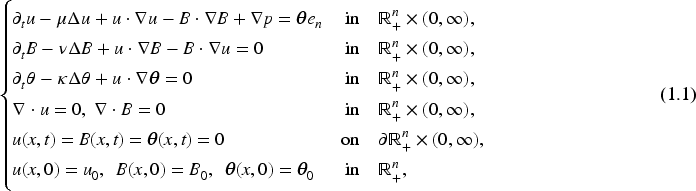
We consider the time decay estimates of solutions to the viscous incompressible magnetic Bénard system in a half-space

\begin{aligned} {\begin{aligned} \partial_{t} u - μ Δ u + u \cdot \nabla u - B \cdot \nabla B + \nabla p = θ e_{n} & in & R_{+}^{n} \times (0, \infty), \\ \partial_{t} B - ν Δ B + u \cdot \nabla B - B \cdot \nabla u = 0 & in & R_{+}^{n} \times (0, \infty), \\ \partial_{t} θ - κ Δ θ + u \cdot \nabla θ = 0 & in & R_{+}^{n} \times (0, \infty), \\ \nabla \cdot u = 0, \nabla \cdot B = 0 & in & R_{+}^{n} \times (0, \infty), \\ u (x, t) = B (x, t) = θ (x, t) = 0 & on & \partial R_{+}^{n} \times (0, \infty), \\ u (x, 0) = u_{0}, B (x, 0) = B_{0}, θ (x, 0) = θ_{0} & in & R_{+}^{n}, \end{aligned} \end{aligned}

(1.1)

where

n \geq 3

, and

R_{+}^{n} = {x = (x^{'}, x_{n}) \in R^{n} ∣ x_{n} > 0}

is the upper half-space of

R^{n}

. The unknown functions

u = (u_{1} (x, t), u_{2} (x, t), \dots, u_{n} (x, t))

B = (B_{1} (x, t), B_{2} (x, t), \dots, B_{n} (x, t))

, and

θ = θ (x, t)

denote the velocity, the magnetic field, and the temperature, respectively,

p = p (x, t)

is the pressure and

e_{n}

is the unit vector. The constants

μ > 0

and

ν > 0

are the coefficients of dissipation and magnetic diffusion, and

κ

characterizes the strength of heat conduction.

The magnetic Bénard system is widely used to model thermal convection dynamics under the influence of a magnetic field (see Fan et al., 2019; Rionero, 1998), which is derived from the magnetohydrodynamic (MHD) equations by introducing the Boussinesq approximation. This simplified model confines and restricts the effects arising from density variations to the buoyancy term, thus preserving the interplay between gravitational and magnetic forces.

In the absence of magnetic field and temperature effects, the equations in (1.1) reduce to the incompressible Navier–Stokes equations. There is a great literature to date on the existence and time decay estimates of solutions to the incompressible Navier–Stokes equations. Leray (1934) first established the existence of global weak solutions to the three-dimensional Navier–Stokes equations in the whole space, though without addressing the decay and regularity properties of these weak solutions. Based on the strong $L^{p}$ -solution theory, Kato (1984) proved that for $n \leq 4$ , the $L^{2}$ -norm of weak solutions vanishes as time tends to infinity, pioneering research into decay rates. To determine the decay rate of weak solutions in a three-dimensional space, Schonbek (1992, 1995) introduced the Fourier-splitting method and extended the results to higher-order norms decay (Schonbek & Wiegner, 1996). Notably, the whole-space Fourier-transform techniques are inapplicable to half-spaces. Using the Stokes operator fractional power estimates, Borchers and Miyakawa (1988) first derived $L^{2}$ -decay of solutions to Navier–Stokes flow in the half-space. Later, Bae and Choe (2001) refined the precision of the time decay rate through the Stokes solution formula. It is also well known that in higher space dimensions, the existence of regular solutions can only be proved when the initial data satisfies the smallness assumption within a specific function space (Lemarié, 2002). There are relatively few results on $L^{q}$ ( $1 \leq q \leq \infty$ ) estimates for solutions to the Navier–Stokes equations in the half-space and general unbounded domains. Han (2010, 2011, 2012) investigated the solutions of the incompressible Stokes equations and Navier–Stokes equations in half-spaces, along with the decay properties of their spatial derivatives of all orders, deriving specific decay rate estimates in the $L^{q} (1 \leq q \leq \infty)$ space. Liu (2020) studied the decay of weak solutions to three-dimensional Navier–Stokes equations in general unbounded domains and derived explicit $L^{2}$ -decay rates as $t ⟶ \infty$ . Han (2024) has recently achieved significant progress in this field, establishing the $L^{1}$ -decay behavior of higher-order norms for solutions to the Navier–Stokes equations in the upper half-space, which provides a crucial reference for analyzing higher-order decay behavior in $L^{1}$ .

In recent years, the existence, regularity, and decay estimates of solutions to the magnetic Bénard system have attracted considerable attention. The classical decay results for related models, including the Navier–Stokes equations and the Boussinesq equations, provide crucial theoretical references and methodological implications (see, e.g., Brandolese, 2004; Brandolese & Schonbek, 2012; Cannone et al., 2000; Chen & Wang, 2024; Fujigaki & Miyakawa, 2001; Kato, 1984; Kozono & Ogawa, 1992; Liu, 2019; Schonbek, 1992). For the magnetic Bénard system itself, significant advancements have been made concerning the global existence and the regularity criteria of weak solutions, with relevant conclusions presented in Abidi, Gui, et al. (2011), He and Xin (2005), and Regmi and Sharma (2019). With a small assumption about the initial data, strong solutions have also been investigated in Huang (2023), Li (2024), Li et al. (2022), Li and Wang (2020), Luo et al. (2025), and Pan (2022). Additionally, for special initial conditions, particularly axisymmetric data, the specific impact of initial configurations on enhancing solution regularity and damping rates has been investigated in Abidi, Hmidi, et al. (2011), Hmidi and Rousset (2010), and Pan (2022).

As far as we know, relatively few mathematical results exist regarding time decay estimates for solutions of the magnetic Bénard system in the half-space and general unbounded domains. Inspired by the $L^{q} - L^{r}$ estimates developed by Han (2022), Han and Schonbek (2014), and Han (2024) for the Navier–Stokes equations and Boussinesq system in the half-space, as well as the spectral analysis and energy estimate methods employed by Liu (2019), Liu and Yu (2015), and Liu and Han (2024) for MHD flows in general domains, the main aim of this paper is to systematically explore the time decay estimates of weak and strong solutions to problem (1.1).

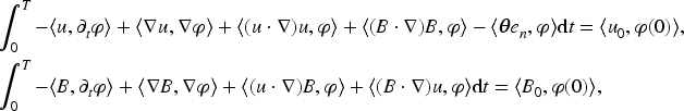
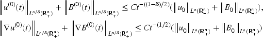
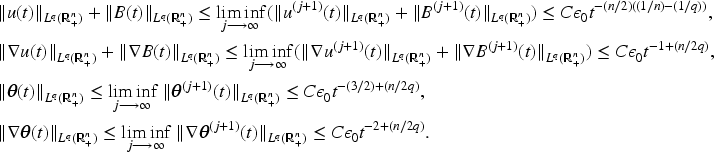
Without loss of generality, we assume $μ = ν = κ = 1$ . Our main results are stated as follows. The first result establishes the $L^{2}$ -decay for weak solutions of the magnetic Bénard system in the half-space.

Theorem 1.1

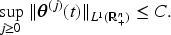
Let $u_{0}, B_{0} \in L_{σ}^{2} (R_{+}^{n})$ and $θ_{0} \in L^{1} (R_{+}^{n}) \cap L^{2} (R_{+}^{n})$ , $n \geq 3$ . Then, problem (1.1) admits a weak solution $(u, B, θ)$ satisfying for $t > 0$

\begin{aligned} {‖ θ (t) ‖}_{L^{2} (R_{+}^{n})} \leq C (1 + t)^{- (n / 4)} \end{aligned}

(1.2)

and

\begin{aligned} {‖ u (t) ‖}_{L^{2} (R_{+}^{n})} + {‖ B (t) ‖}_{L^{2} (R_{+}^{n})} \leq {\begin{cases} C (1 + t)^{1 / 4} & if n = 3, \\ C \log_{e} (1 + t) & if n = 4, \\ C & if n \geq 5. \end{cases} \end{aligned}

(1.3)

If there exists

δ > 0

depending on

‖ u_{0} ‖_{L^{2} (R_{+}^{n})}

, such that

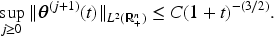
\begin{aligned} ‖ θ_{0} ‖_{L^{1} (R_{+}^{n})} \leq δ for n = 3 and ‖ x_{n} θ_{0} ‖_{L^{1} (R_{+}^{n})} < \infty for n \geq 4 \end{aligned}

(1.4)

holds, then the weak solution

(u, B, θ)

satisfies

\begin{aligned} {‖ θ (t) ‖}_{L^{2} (R_{+}^{n})} \leq C (1 + t)^{- ((n + 2) / 4)}, \forall t > 0 \end{aligned}

(1.5)

and

\begin{aligned} {‖ u (t) ‖}_{L^{2} (R_{+}^{n})} + {‖ B (t) ‖}_{L^{2} (R_{+}^{n})} ⟶ 0 as t ⟶ + \infty . \end{aligned}

(1.6)

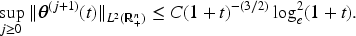
Further, if

u_{0}, B_{0} \in L^{(n / (n - 1))} (R_{+}^{n})

, then for any small

ϵ > 0

and

t > 0

, it holds that

\begin{aligned} {‖ u (t) ‖}_{L^{2} (R_{+}^{n})} + {‖ B (t) ‖}_{L^{2} (R_{+}^{n})} \leq C_{ϵ} (1 + t)^{- ((n - 2) / 4) + ϵ} . \end{aligned}

(1.7)

The $L^{q}$ estimates of solutions to the Navier–Stokes equations have been obtained (see, e.g., Fujigaki & Miyakawa, 2001; Han, 2010, 2011), but establishing the $L^{q}$ -decay estimates of solutions to problem (1.1) is typically more challenging and less common. The following Theorems 1.2 and 1.3 focus on the $L^{q}$ -decay estimates of solutions to problem (1.1) under the assumption on the small initial data condition and the weighted initial data, respectively.

Theorem 1.2

Let $u_{0}, B_{0} \in L_{σ}^{n} (R_{+}^{n})$ , and $θ_{0} \in L^{n / 3} (R_{+}^{n})$ , $n \geq 3$ . There exists $ϵ_{0} > 0$ sufficiently small such that if $‖ u_{0} ‖_{L^{n} (R_{+}^{n})} + ‖ B_{0} ‖_{L^{n} (R_{+}^{n})} + ‖ θ_{0} ‖_{L^{n / 3} (R_{+}^{n})} \leq ϵ_{0}$ , then problem (1.1) admits a strong solution $(u, B, θ)$ satisfying for $t > 0$ . Moreover, the solution satisfies that

\begin{aligned} ‖ \nabla^{k} u (t) ‖_{L^{q} (R_{+}^{n})} + ‖ \nabla^{k} B (t) ‖_{L^{q} (R_{+}^{n})} \leq C ϵ_{0} t^{- (k / 2) - (n / 2) ((1 / n) - (1 / q))} for k = 0, 1 and n \leq q \leq \infty, \\ ‖ \nabla^{k} θ (t) ‖ y_{L^{q} (R_{+}^{n})} \leq C ϵ_{0} t^{- (k / 2) - 1 - (n / 2) ((1 / n) - (1 / q))} for k = 0, 1 and n \leq q \leq \infty . \end{aligned}

Theorem 1.3

Let $u_{0}, B_{0} \in L_{σ}^{n} (R_{+}^{n}) \cap L^{(n / (n - 1))} (R_{+}^{n})$ , and $θ_{0} \in L^{1} (R_{+}^{n}) \cap L^{2} (R_{+}^{n}) \cap L^{n / 3} (R_{+}^{n})$ , $n \geq 3$ . Assume (1.4) holds. Let $(u, B, θ)$ be the strong solution to problem (1.1) obtained in Theorem 1.2. Then, for $t > 0$ , it holds that

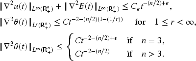
\begin{aligned} [‖ \nabla^{k} u (t) ‖_{L^{q} (R_{+}^{n})} + ‖ \nabla^{k} B (t) ‖_{L^{q} (R_{+}^{n})} \leq C t^{- ((k - 1) / 2) - (n / 2) (1 - (1 / q))} for k = 0, 1 and \frac{n}{n - 1} \leq q \leq \infty, \\ ‖ \nabla^{k} θ (t) ‖_{L^{q} (R_{+}^{n})} \leq C t^{- ((k + 1) / 2) - (n / 2) (1 - (1 / q))} for k = 0, 1 and 1 \leq q \leq \infty . \end{aligned}

Building on the foundational research of Schonbek and Wiegner (1996) for the Navier–Stokes equations in the whole space, and Han and Schonbek (2014) for the Boussinesq system in the half-space, the following theorem establishes decay estimates of the second-order derivatives of the strong solution to problem (1.1). The decay estimates of the third-order derivatives of the temperature are also established under additional conditions.

Theorem 1.4

‖ \nabla^{2} u (t) ‖_{L^{r} (R_{+}^{n})} + ‖ \nabla^{2} B (t) ‖_{L^{r} (R_{+}^{n})} + {‖ \partial_{t} u (t) ‖}_{L^{r} (R_{+}^{n})} + {‖ \partial_{t} B (t) ‖}_{L^{r} (R_{+}^{n})} + {‖ \nabla p (t) ‖}_{L^{r} (R_{+}^{n})} \leq C t^{- (1 / 2) - (n / 2) (1 - (1 / r))},

provided that

n / (n - 1) \leq r < \infty

, and

‖ \nabla^{2} θ (t) ‖_{L^{r} (R_{+}^{n})} \leq C t^{- (3 / 2) - (n / 2) (1 - (1 / r))} for 1 \leq r \leq \infty .

Further, if

y_{n} θ_{0}, y_{n}^{2} θ_{0} \in L^{1} (R_{+}^{n})

, and

y_{n} θ_{0} \in L^{\infty} (R_{+}^{n})

, then for any sufficiently small number

ϵ > 0

and

t \geq 1

, it holds that

\begin{aligned} ‖ \nabla^{2} u (t) ‖_{L^{\infty} (R_{+}^{n})} + ‖ \nabla^{2} B (t) ‖_{L^{\infty} (R_{+}^{n})} \leq C_{ϵ} t^{- (n / 2) + ϵ}, \\ ‖ \nabla^{3} θ (t) ‖_{L^{r} (R_{+}^{n})} \leq C t^{- 2 - (n / 2) (1 - (1 / r))} for 1 \leq r < \infty, \\ ‖ \nabla^{3} θ (t) ‖_{L^{\infty} (R_{+}^{n})} \leq {\begin{cases} C t^{- 2 - (n / 2) + ϵ} & if n = 3, \\ C t^{- 2 - (n / 2)} & if n > 3. \end{cases} \end{aligned}

The structure of this paper is organized as follows: In Section 1, the required background and main findings are introduced. Section 2 discusses some inequalities. In Section 3, we present the decay behaviors of weak and strong solutions to problem (1.1). Finally, Section 4 focuses on establishing the estimates of the second-order derivatives of the strong solution and the third-order derivatives of the temperature field to problem (1.1).

2. Preliminaries

In this section, we list some notations and several inequalities that are frequently employed in this work.

Notation. We denote the usual $L^{q}$ spaces by

L^{q} (R_{+}^{3}) = {f (x) ∣ ‖ f (x) ‖_{L^{q} (R_{+}^{n})} < \infty}, 1 \leq q \leq \infty .

The

L^{\infty} (R_{+}^{n})

norm is given by

‖ u ‖_{L^{\infty} (R_{+}^{n})} = ess sup_{x \in R_{+}^{n}} | u (x) | .

And we denote by

C_{0, σ}^{\infty} (R_{+}^{n})

the set of all

C^{\infty}

divergence-free vector fields with compact support in

R_{+}^{n} .

The space

L_{σ}^{q} (R_{+}^{n}) (1 < q < \infty)

is the closure of

C_{0, σ}^{\infty} (R_{+}^{n})

with respect to

‖ \cdot ‖_{L}^{q} (R_{+}^{n})

, namely

L_{σ}^{q} (R_{+}^{n}) = {ϕ = (ϕ_{1}, ϕ_{2}, \dots, ϕ_{n}) \in L^{q} (R_{+}^{n}) ∣ \nabla \cdot ϕ = 0} .

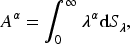
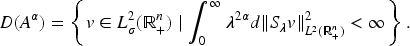
Then, we recall some facts about the Stokes operator $A$ . The Stokes operator $A$ is defined by $A = - P Δ : D (A) \to L_{σ}^{2} (R_{+}^{n})$ be the Stokes operator for $R_{+}^{n}$ , $P : L^{2} (R_{+}^{n}) \to L_{σ}^{2} (R_{+}^{n})$ is the Helmholtz projection operator. Let $A$ is self-adjoint and dense defined on $L_{σ}^{2} (R_{+}^{n})$ . By the spectral theorem, there exists a uniquely determined spectral resolution ${S_{λ} | λ \geq 0}$ in $L_{σ}^{2} (R_{+}^{n})$ . The operator $A^{α}$ , for $0 < α \leq 1$ , is then defined as follows:

A^{α} = \int_{0}^{\infty} λ^{α} d S_{λ},

with domain

D (A^{α}) = {v \in L_{σ}^{2} (R_{+}^{n}) ∣ \int_{0}^{\infty} λ^{2 α} d ‖ S_{λ} v ‖_{L^{2} (R_{+}^{n})}^{2} < \infty} .

Definition 2.1
$(u, B, θ)$ is a weak solution to problem (1.1) if

(i)
$u, B \in L^{\infty} (0, T; L_{σ}^{2} (R_{+}^{n})) \cap L^{2} (0, T; H_{0}^{1} (R_{+}^{n})), θ \in L^{\infty} (0, T; L^{2} (R_{+}^{n})) \cap L^{2} (0, T; H_{0}^{1} (R_{+}^{n}))$
(ii)
$u, B, θ$ satisfy the weak forms
$\begin{aligned} \int_{0}^{T} - ⟨ u, \partial_{t} φ ⟩ + ⟨ \nabla u, \nabla φ ⟩ + ⟨ (u \cdot \nabla) u, φ ⟩ + ⟨ (B \cdot \nabla) B, φ ⟩ - ⟨ θ e_{n}, φ ⟩ d t = ⟨ u_{0}, φ (0) ⟩, \\ \int_{0}^{T} - ⟨ B, \partial_{t} φ ⟩ + ⟨ \nabla B, \nabla φ ⟩ + ⟨ (u \cdot \nabla) B, φ ⟩ + ⟨ (B \cdot \nabla) u, φ ⟩ d t = ⟨ B_{0}, φ (0) ⟩, \end{aligned}$
for all text functions $φ \in C_{0}^{\infty} ([0, T); C_{0, σ}^{\infty} (R_{+}^{n}))$ , and
$\int_{0}^{T} - ⟨ θ, \partial_{t} ψ ⟩ + ⟨ \nabla θ, \nabla ψ ⟩ + ⟨ (u \cdot \nabla) θ, ψ ⟩ d t = ⟨ θ_{0}, ψ (0) ⟩,$
for all text functions $ψ \in C_{0}^{\infty} ([0, T); C_{0}^{\infty} (R_{+}^{n}))$ .

Remark 2.2
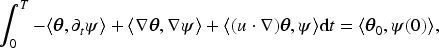
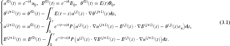
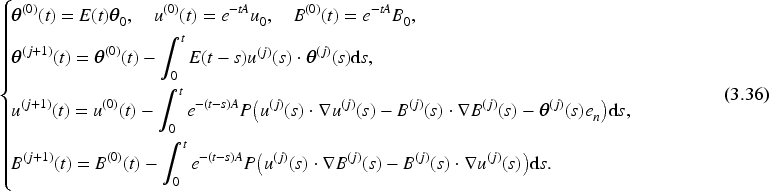
We intend to establish the algebraic decay estimates of the weak and strong solutions. To solve this problem, we usually invoke the projector P, transform problem (1.1) into the following integral forms by Duhamel’s formula:
$\begin{aligned} {\begin{cases} u (t) = e^{- t A} u_{0} - \int_{0}^{t} e^{- (t - s) A} P (u (s) \cdot \nabla u (s) - B (s) \cdot \nabla B (s) - θ (s) e_{n}) d s, \\ B (t) = e^{- t A} B_{0} - \int_{0}^{t} e^{- (t - s) A} P (u (s) \cdot \nabla B (s) - B (s) \cdot \nabla u (s)) d s, \\ θ (t) = E (t) θ_{0} - \int_{0}^{t} E (t - s) u (s) \cdot \nabla θ (s) d s, \end{cases} \end{aligned}$
(2.1)
where $u, B \in L^{\infty} (0, T; L_{σ}^{2} (R_{+}^{n})) \cap L^{2} (0, T; H_{0}^{1} (R_{+}^{n})), and θ \in L^{\infty} (0, T; L^{2} (R_{+}^{n})) \cap L^{2} (0, T; H_{0}^{1} (R_{+}^{n})),$ the operators $E (t)$ is given in (3.2).
Remark 2.3
A weak solution $(u, B, θ)$ is called a strong solution if $u, B \in L^{\infty} (0, T; L_{σ}^{2} (R_{+}^{n})) \cap L^{2} (0, T; H_{0}^{1} (R_{+}^{n})), and θ \in L^{\infty} (0, T; L^{2} (R_{+}^{n})) \cap L^{2} (0, T; H_{0}^{1} (R_{+}^{n}))$ . Further, it can be demonstrated that a strong solution is in fact classical by combining the regularity criteria for the Navier–Stokes equations with standard regularity theory for parabolic equations. This implies that it not only satisfies the weak integral form but also possesses sufficient smoothness.
Lemma 2.4 Fujigaki & Miyakawa, 2001

For any $f \in L_{σ}^{q} (R_{+}^{n})$ ,

‖ \nabla^{k} e^{- t A} f ‖_{L^{r} (R_{+}^{n})} \leq C t^{- (k / 2) - (n / 2) ((1 / q) - (1 / r))} ‖ f ‖_{L^{q} (R_{+}^{n})},

with

k = 0, 1, \dots

, provided that

1 \leq q < r \leq \infty

1 < q \leq r \leq \infty

Lemma 2.5 Han, 2012

Let $1 < q < \infty$ . Assume that $f \in W^{1, q} (R_{+}^{n}) satisfies \nabla \cdot f = 0 in R_{+}^{n} and f_{n} |_{\partial_{R_{+}^{n}}} = 0$ . Then, for any $0 < δ < 1$ and $t > 0$

‖ \nabla^{2} e^{- t A} f ‖_{L^{\infty} (R_{+}^{n})} \leq C (t^{- (1 / 2) - (n / 2 q)} {‖ \nabla f ‖}_{L^{q} (R_{+}^{n})} + t^{- 1 + δ / 2 - (n / 2 q)} ‖ y_{n}^{- δ} f ‖_{L^{q} (R_{+}^{n})}) .

Lemma 2.6 Brandolese, 2004

Let $(u_{0}, B_{0}, θ_{0}) \in L_{σ}^{2} \times L_{σ}^{2} \times L^{2}$ and let $(u, B, θ)$ be the solution to system (1.1). Assume that $1 \leq p < \infty$ . If $θ_{0} \in L^{1} \cap L^{p}$ , then

sup_{j \geq 0} ‖ θ^{(j + 1)} (t) ‖_{L^{q} (R_{+}^{n})} \leq ‖ θ_{0} ‖_{L^{1} (R_{+}^{n})} {(A + \frac{C t}{q})}^{- (n / 2) (1 - (1 / q))},

where

A = A (q, ‖ θ_{0} ‖_{L^{1} (R_{+}^{n})}, ‖ θ_{0} ‖_{L^{q} (R_{+}^{n})})

and

C > 0

is an absolute constant.

Lemma 2.7 Borchers & Miyakawa, 1988

For all $λ > 0 and w, u \in H_{0, σ}^{1} (R_{+}^{n})$

‖ S_{λ} P (w \cdot \nabla) u ‖_{L^{2} (R_{+}^{n})} \leq C λ^{(n + 2) / 4} ‖ w ‖_{L^{2} (R_{+}^{n})} ‖ u ‖_{L^{2} (R_{+}^{n})},

where C is independent of

w, u, and λ

Lemma 2.8 Han, 2010, 2012

Let $0 \leq η < 1, 1 \leq k \leq n, and 1 \leq q \leq \infty$ . Then, for any $u, v \in C_{0, σ}^{\infty} (R_{+}^{n})$

{‖ \sum_{i, j = 1}^{n} x_{n}^{- η} \nabla N \partial_{i} \partial_{j} (u_{i} v_{j}) ‖}_{L^{q} (R_{+}^{n})} \leq C ({‖ u ‖}_{L^{2 q} (R_{+}^{n})}^{2} + {‖ v ‖}_{L^{2 q} (R_{+}^{n})}^{2} + {‖ \nabla u ‖}_{L^{2 q} (R_{+}^{n})}^{2} + {‖ \nabla v ‖}_{L^{2 q} (R_{+}^{n})}^{2}),

and for any

θ \in C_{0}^{\infty} (R_{+}^{n})

‖ x_{n}^{- η} \nabla N div (e_{n} θ) ‖_{L^{q} (R_{+}^{n})} \leq C ({‖ y_{n} θ ‖}_{L^{q} (R_{+}^{n})} + {‖ \partial_{n} θ ‖}_{L^{q} (R_{+}^{n})}) .

Lemma 2.9 Han, 2011; Liu, 2019

Let $1 \leq q \leq \infty, 1 \leq i, j \leq n$ . Then, for any $u, v \in C_{0, σ}^{\infty} (R_{+}^{n})$

\begin{aligned} {‖ \sum_{i, j = 1}^{n} \nabla^{2} N \partial_{i} \partial_{j} (u_{i} v_{j}) ‖}_{L^{q} (R_{+}^{n})} & \leq C ({‖ u ‖}_{L^{2 q} (R_{+}^{n})}^{2} + {‖ v ‖}_{L^{2 q} (R_{+}^{n})}^{2} + {‖ \nabla u ‖}_{L^{2 q} (R_{+}^{n})}^{2} + {‖ \nabla v ‖}_{L^{2 q} (R_{+}^{n})}^{2} \\ + ‖ \nabla^{2} u ‖_{L^{2 q} (R_{+}^{n})}^{2} + ‖ \nabla^{2} v ‖_{L^{2 q} (R_{+}^{n})}^{2}), \end{aligned}

and for any

θ \in C_{0}^{\infty} (R_{+}^{n})

‖ \nabla^{2} N div (e_{n} θ) ‖_{L^{q} (R_{+}^{n})} \leq C ({‖ θ ‖}_{L^{q} (R_{+}^{n})} + ‖ \nabla^{2} θ ‖_{L^{q} (R_{+}^{n})}) .

3. Decay Rates of Weak and Strong Solutions

This section is devoted to prove investigating the decay behaviors of weak and strong solutions to problem (1.1). First, we establish the existence and basic decay properties of weak solutions, we then construct strong solutions with small initial data, and finally, further investigate the decay behavior of strong solutions when no small initial conditions are applied.

3.1. $L^{2}$ -Decay of Weak Solutions

In this subsection, our primary goal is to analyze the decay behavior of weak solutions to problem (1.1) within the $L^{2}$ space.

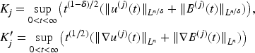
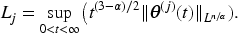
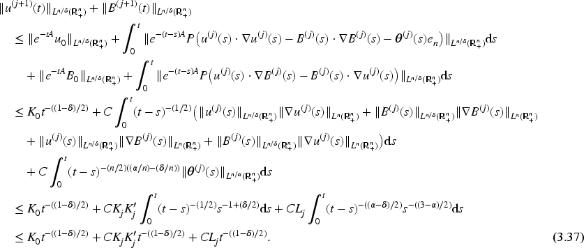
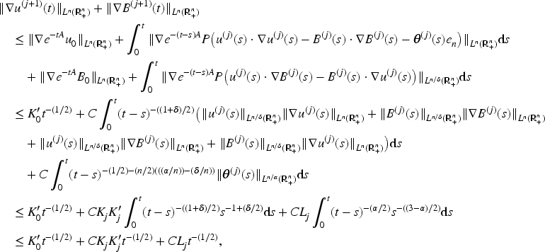
Proof of Theorem 1.1 Let $u_{0}, B_{0} \in L_{σ}^{2} (R_{+}^{n})$ , and $θ_{0} \in L^{1} (R_{+}^{n}) \cap L^{2} (R_{+}^{n})$ , we analyze the iterative approximation for $0 \leq t < \infty$ , $j = 0, 1, 2 \dots$

\begin{aligned} {\begin{cases} u^{(0)} (t) = e^{- t A} u_{0}, B^{(0)} (t) = e^{- t A} B_{0}, θ^{(0)} (t) = E (t) θ_{0}, \\ θ^{(j + 1)} (t) = θ^{(0)} (t) - \int_{0}^{t} E (t - s) u^{(j)} (s) \cdot \nabla θ^{(j + 1)} (s) d s, \\ u^{(j + 1)} (t) = u^{(0)} (t) - \int_{0}^{t} e^{- (t - s) A} P (u^{(j)} (s) \cdot \nabla u^{(j + 1)} (s) - B^{(j)} (s) \cdot \nabla B^{(j + 1)} (s) - θ^{(j)} (s) e_{n}) d s, \\ B^{(j + 1)} (t) = B^{(0)} (t) - \int_{0}^{t} e^{- (t - s) A} P (u^{(j)} (s) \cdot \nabla B^{(j + 1)} (s) - B^{(j)} (s) \cdot \nabla u^{(j + 1)} (s)) d s . \end{cases} \end{aligned}

(3.1)

The operator

E (t)

is defined for

n \geq 3

as follows

\begin{aligned} E (t) f (x) = \int_{R_{+}^{n}} [G_{t} (x^{'} - y^{'}, x_{n} - y_{n}) - G_{t} (x^{'} - y^{'}, x_{n} + y_{n})] f (y) d y \end{aligned}

(3.2)

and

G_{t} (x) = (4 π t)^{- (n / 2)} e^{- (| x |^{2} / 4 t)}

is the Gauss kernel. It can be concluded that problem (3.1) admits a unique strong solution

(θ^{(j + 1)}, u^{(j + 1)}, B^{(j + 1)})

(see Borchers & Miyakawa, 1988). We have a simple calculation:

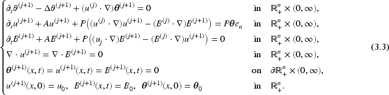
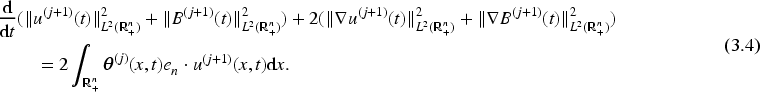
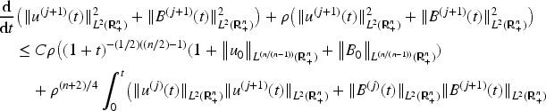
\begin{aligned} {\begin{aligned} \partial_{t} θ^{(j + 1)} - Δ θ^{(j + 1)} + (u^{(j)} \cdot \nabla) θ^{(j + 1)} = 0 & in & R_{+}^{n} \times (0, \infty), \\ \partial_{t} u^{(j + 1)} + A u^{(j + 1)} + P ((u^{(j)} \cdot \nabla) u^{(j + 1)} - (B^{(j)} \cdot \nabla) B^{(j + 1)}) = P θ e_{n} & in & R_{+}^{n} \times (0, \infty), \\ \partial_{t} B^{(j + 1)} + A B^{(j + 1)} + P ((u_{j} \cdot \nabla) B^{(j + 1)} - (B^{(j)} \cdot \nabla) u^{(j + 1)}) = 0 & in & R_{+}^{n} \times (0, \infty), \\ \nabla \cdot u^{(j + 1)} = \nabla \cdot B^{(j + 1)} = 0 & in & R_{+}^{n} \times (0, \infty), \\ θ^{(j + 1)} (x, t) = u^{(j + 1)} (x, t) = B^{(j + 1)} (x, t) = 0 & on & \partial R_{+}^{n} \times (0, \infty), \\ u^{(j + 1)} (x, 0) = u_{0}, B^{(j + 1)} (x, t) = B_{0}, θ^{(j + 1)} (x, 0) = θ_{0} & in & R_{+}^{n} . \end{aligned} \end{aligned}

(3.3)

Multiplying the second and third equations of (3.3) by

u^{(j + 1)}

and

B^{(j + 1)}

, then integrating over

R_{+}^{n}

and adding the two results together to obtain

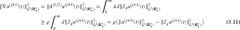
\begin{aligned} \begin{aligned} \frac{d}{d t} (‖ u^{(j + 1)} (t) ‖_{L^{2} (R_{+}^{n})}^{2} + ‖ B^{(j + 1)} (t) ‖_{L^{2} (R_{+}^{n})}^{2}) + 2 (‖ \nabla u^{(j + 1)} (t) ‖_{L^{2} (R_{+}^{n})}^{2} + ‖ \nabla B^{(j + 1)} (t) ‖_{L^{2} (R_{+}^{n})}^{2}) \\ = 2 \int_{R_{+}^{n}} θ^{(j)} (x, t) e_{n} \cdot u^{(j + 1)} (x, t) d x . \end{aligned} \end{aligned}

(3.4)

Multiply the first equation of (3.3) by

θ^{(j + 1)}

and also integrate the result over

R_{+}^{n}

, then we have for

j = 0, 1, 2 \dots

and

t > 0

\begin{aligned} \frac{d}{d t} ‖ θ^{(j + 1)} (t) ‖_{L^{2} (R_{+}^{n})}^{2} + 2 ‖ \nabla θ^{(j + 1)} (t) ‖_{L^{2} (R_{+}^{n})}^{2} = 0. \end{aligned}

(3.5)

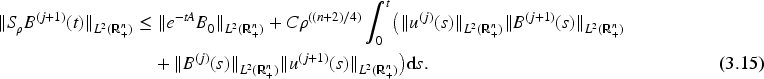
By Lemma 2.6, we get $sup_{j \geq 0} ‖ θ^{(j + 1)} (t) ‖_{L^{2} (R_{+}^{n})} \leq C ‖ θ_{0} ‖_{L^{1} (R_{+}^{n})} (1 + t)^{- (n / 4)}$ . In addition, based on the operator $E (t)$ , we infer for $t > 0$

\begin{aligned} ‖ θ^{(0)} (t) ‖_{L^{2} (R_{+}^{n})} = ‖ E (t) θ_{0} ‖_{L^{2} (R_{+}^{n})} \leq C ‖ θ_{0} ‖_{L^{1} (R_{+}^{n})} (1 + t)^{- (n / 4)} . \end{aligned}

(3.6)

Thus, for all

t > 0

\begin{aligned} sup_{j \geq 0} ‖ θ^{(j)} (t) ‖_{L^{2} (R_{+}^{n})} \leq C (1 + t)^{- (n / 4)} . \end{aligned}

(3.7)

From (3.4), we arrive at

\begin{aligned} \frac{d}{d t} (‖ u^{(j + 1)} (t) ‖_{L^{2} (R_{+}^{n})}^{2} + ‖ B^{(j + 1)} (t) ‖_{L^{2} (R_{+}^{n})}^{2}) \leq 2 ‖ u^{(j + 1)} (t) ‖_{L^{2} (R_{+}^{n})} ‖ θ^{(j)} (t) ‖_{L^{2} (R_{+}^{n})} . \end{aligned}

(3.8)

By Lemma 2.4, it follows that for $t > 0$

\begin{aligned} \begin{aligned} ‖ u^{(0)} (t) ‖_{L^{2} (R_{+}^{n})} = ‖ e^{- t A} u_{0} ‖_{L^{2} (R_{+}^{n})} \leq C {‖ u_{0} ‖}_{L^{2} (R_{+}^{n})}, \\ ‖ B^{(0)} (t) ‖_{L^{2} (R_{+}^{n})} = ‖ e^{- t A} B_{0} ‖_{L^{2} (R_{+}^{n})} \leq C {‖ B_{0} ‖}_{L^{2} (R_{+}^{n})} . \end{aligned} \end{aligned}

(3.9)

Thus, combining this with the earlier estimates and taking

C ε < 1

, we obtain

\begin{aligned} ‖ u^{(j + 1)} (t) ‖_{L^{2} (R_{+}^{n})}^{2} + ‖ B^{(j + 1)} (t) ‖_{L^{2} (R_{+}^{n})}^{2} & \leq C \int_{0}^{t} ‖ u^{(j + 1)} (s) ‖_{L^{2} (R_{+}^{n})} ‖ θ^{(j)} (s) ‖_{L^{2} (R_{+}^{n})} d s \\ \leq C sup_{j \geq 0} ‖ u^{(j + 1)} (t) ‖_{L^{2} (R_{+}^{n})} \int_{0}^{t} (1 + s)^{- (n / 4)} d s \\ \leq C ε sup_{j \geq 0} (‖ u^{(j + 1)} (t) ‖_{L^{2} (R_{+}^{n})}^{2} + ‖ B^{(j + 1)} (t) ‖_{L^{2} (R_{+}^{n})}^{2}) \\ + C (ε) {\begin{cases} (1 + t)^{(1 / 2)} & if n = 3, \\ \log_{e}^{2} (1 + t) & if n = 4, \\ 1 & if n \geq 5, \end{cases} \end{aligned}

which implies that

\begin{aligned} \begin{aligned} sup_{j \geq 0} (‖ u^{(j + 1)} (t) ‖_{L^{2} (R_{+}^{n})} + ‖ B^{(j + 1)} (t) ‖_{L^{2} (R_{+}^{n})}) \leq {\begin{cases} C (1 + t)^{1 / 4} & if n = 3, \\ C \log_{e} (1 + t) & if n = 4, \\ C & if n \geq 5, \end{cases} \end{aligned} \end{aligned}

(3.10)

where

C

depends on

n, ε, ‖ u_{0} ‖_{L^{2} (R_{+}^{n})}, ‖ B_{0} ‖_{L^{2} (R_{+}^{n})}, and ‖ θ_{0} ‖_{L^{1} (R_{+}^{n})}

. This completes the proof of (1.2) and (1.3).□

Based on assumption (1.4), the following auxiliary estimate

\begin{aligned} ‖ \nabla u^{(j + 1)} (t) ‖_{L^{2} (R_{+}^{n})}^{2} & = ‖ A^{(1 / 2)} u^{(j + 1)} (t) ‖_{L^{2} (R_{+}^{n})}^{2} = \int_{0}^{\infty} λ d ‖ S_{λ} u^{(j + 1)} (t) ‖_{L^{2} (R_{+}^{n})}^{2} \\ \geq ρ \int_{ρ}^{\infty} d ‖ S_{λ} u^{(j + 1)} (t) ‖_{L^{2} (R_{+}^{n})}^{2} = ρ (‖ u^{(j + 1)} (t) ‖_{L^{2} (R_{+}^{n})}^{2} - ‖ S_{ρ} u^{(j + 1)} (t) ‖_{L^{2} (R_{+}^{n})}^{2}) \end{aligned}

(3.11)

holds, which will be used in the proof of the second part of Theorem 1.1.

Similarly, we have

\begin{aligned} ‖ \nabla B^{(j + 1)} (t) ‖_{L^{2} (R_{+}^{n})}^{2} \geq ρ (‖ B^{(j + 1)} (t) ‖_{L^{2} (R_{+}^{n})}^{2} - ‖ S_{ρ} B^{(j + 1)} (t) ‖_{L^{2} (R_{+}^{n})}^{2}) . \end{aligned}

(3.12)

Inserting (3.11) and (3.12) into (3.4), we obtain

\begin{aligned} \frac{d}{d t} (‖ u^{(j + 1)} (t) ‖_{L^{2} (R_{+}^{n})}^{2} + ‖ B^{(j + 1)} (t) ‖_{L^{2} (R_{+}^{n})}^{2}) + ρ (‖ u^{(j + 1)} (t) ‖_{L^{2} (R_{+}^{n})}^{2} + ‖ B^{(j + 1)} (t) ‖_{L^{2} (R_{+}^{n})}^{2}) \\ \leq 2 ρ (‖ S_{ρ} u^{(j + 1)} (t) ‖_{L^{2} (R_{+}^{n})}^{2} + ‖ S_{ρ} B^{(j + 1)} (t) ‖_{L^{2} (R_{+}^{n})}^{2}) + 2 ‖ u^{(j + 1)} (t) ‖_{L^{2} (R_{+}^{n})} ‖ θ^{(j)} (t) ‖_{L^{2} (R_{+}^{n})} . \end{aligned}

(3.13)

Combining (3.1) and Lemmas 2.4 and 2.7 yields for any

ρ > 0 and t > 0, 1 < r < 2

\begin{aligned} ‖ S_{ρ} u^{(j + 1)} (t) ‖_{L^{2} (R_{+}^{n})} \\ \leq ‖ S_{ρ} e^{- t A} u_{0} ‖_{L^{2} (R_{+}^{n})} + \int_{0}^{t} ‖ S_{ρ} e^{- (t - s) A} P (e_{n} θ^{(j)} (s)) ‖_{L^{2} (R_{+}^{n})} d s \\ + {‖ \int_{0}^{t} S_{ρ} \int_{0}^{\infty} e^{- (t - s) λ} d [S_{λ} P ((u^{(j)} (s) \cdot \nabla) u^{(j + 1)} (s) - (B^{(j)} (s) \cdot \nabla) B^{(j + 1)} (s))] d s ‖}_{L^{2} (R_{+}^{n})} \\ \leq ‖ e^{- t A} u_{0} ‖_{L^{2} (R_{+}^{n})} + \int_{0}^{t} ‖ S_{ρ} e^{- (t - s) A} P (e_{n} θ^{(j)} (s)) ‖_{L^{2} (R_{+}^{n})} d s \\ + {‖ \int_{0}^{t} (\int_{0}^{ρ} + \int_{ρ}^{\infty}) e^{- (t - s) λ} d [S_{λ} S_{ρ} P ((u^{(j)} (s) \cdot \nabla) u^{(j + 1)} (s) - (B^{(j)} (s) \cdot \nabla) B^{(j + 1)} (s))] d s ‖}_{L^{2} (R_{+}^{n})} \\ \leq ‖ e^{- t A} u_{0} ‖_{L^{2} (R_{+}^{n})} + {‖ \int_{0}^{t} e^{- (t - s) ρ} S_{ρ} P ((u^{(j)} (s) \cdot \nabla) u^{(j + 1)} (s) - (B^{(j)} (s) \cdot \nabla) B^{(j + 1)} (s)) d s ‖}_{L^{2} (R_{+}^{n})} \\ + {‖ \int_{0}^{t} (t - s) {\int_{0}^{ρ} e^{- (t - s) λ} [S_{λ} P ((u^{(j)} (s) \cdot \nabla) u^{(j + 1)} (s) - (B^{(j)} (s) \cdot \nabla) B^{(j + 1)} (s))] d λ} d s ‖}_{L^{2} (R_{+}^{n})} \\ + C \int_{0}^{t / 2} (t - s)^{- (n / 2) (1 / r - (1 / 2))} ‖ θ^{(j)} (s) ‖_{L^{r} (R_{+}^{n})} d s + C \int_{t / 2}^{t} ‖ θ^{(j)} (s) ‖_{L^{2} (R_{+}^{n})} d s \\ \leq ‖ e^{- t A} u_{0} ‖_{L^{2} (R_{+}^{n})} + C ρ^{((n + 2) / 4)} \int_{0}^{t} (‖ u^{(j)} (s) ‖_{L^{2} (R_{+}^{n})} ‖ u^{(j + 1)} (s) ‖_{L^{2} (R_{+}^{n})} + ‖ B^{(j)} (s) ‖_{L^{2} (R_{+}^{n})} ‖ B^{(j + 1)} (s) ‖_{L^{2} (R_{+}^{n})}) d s \\ + \int_{0}^{t / 2} (t - s)^{- (n / 2) (1 / r - (1 / 2))} ‖ θ^{(j)} (s) ‖_{L^{r} (R_{+}^{n})} d s + C \int_{t / 2}^{t} ‖ θ^{(j)} (s) ‖_{L^{2} (R_{+}^{n})} d s . \end{aligned}

(3.14)

Similarly, from (3.1), for any

ρ > 0 and t > 0

, we infer that

\begin{aligned} ‖ S_{ρ} B^{(j + 1)} (t) ‖_{L^{2} (R_{+}^{n})} & \leq ‖ e^{- t A} B_{0} ‖_{L^{2} (R_{+}^{n})} + C ρ^{((n + 2) / 4)} \int_{0}^{t} (‖ u^{(j)} (s) ‖_{L^{2} (R_{+}^{n})} ‖ B^{(j + 1)} (s) ‖_{L^{2} (R_{+}^{n})} \\ + ‖ B^{(j)} (s) ‖_{L^{2} (R_{+}^{n})} ‖ u^{(j + 1)} (s) ‖_{L^{2} (R_{+}^{n})}) d s . \end{aligned}

(3.15)

By combining (3.8), (3.11), and (3.12), it follows that for any

ρ, t > 0 and j = 0, 1, \dots

\begin{aligned} \frac{d}{d t} (‖ u^{(j + 1)} (t) ‖_{L^{2} (R_{+}^{n})}^{2} + ‖ B^{(j + 1)} (t) ‖_{L^{2} (R_{+}^{n})}^{2}) + ρ (‖ u^{(j + 1)} (t) ‖_{L^{2} (R_{+}^{n})}^{2} + ‖ B^{(j + 1)} (t) ‖_{L^{2} (R_{+}^{n})}^{2}) \\ \leq C ρ (‖ e^{- t A} u_{0} ‖_{L^{2} (R_{+}^{n})} + ‖ e^{- t A} B_{0} ‖_{L^{2} (R_{+}^{n})} + ρ^{((n + 2) / 4)} \int_{0}^{t} (‖ u^{(j)} (t) ‖_{L^{2} (R_{+}^{n})} ‖ u^{(j + 1)} (t) ‖_{L^{2} (R_{+}^{n}))} \\ + ‖ B^{(j)} (t) ‖_{L^{2} (R_{+}^{n})} ‖ B^{(j + 1)} (t) ‖_{L^{2} (R_{+}^{n})} + ‖ u^{(j)} (t) ‖_{L^{2} (R_{+}^{n})} ‖ B^{(j + 1)} (t) ‖_{L^{2} (R_{+}^{n})} \\ + ‖ B^{(j)} (t) ‖_{L^{2} (R_{+}^{n})} ‖ u^{(j + 1)} (t) ‖_{L^{2} (R_{+}^{n})}) d s + \int_{0}^{t / 2} (t - s)^{- (n / 2) (1 / r - (1 / 2))} ‖ θ^{(j)} (s) ‖_{L^{1} (R_{+}^{n})}^{(2 / r) - 1} ‖ θ^{(j)} (s) ‖_{L^{2} (R_{+}^{n})}^{2 (1 - (1 / r))} d s \\ + \int_{t / 2}^{t} ‖ θ^{(j)} (s) ‖_{L^{2} (R_{+}^{n})} d s)^{2} + 2 ‖ u^{(j + 1)} (t) ‖_{L^{2} (R_{+}^{n})} ‖ θ^{(j)} (t) ‖_{L^{2} (R_{+}^{n})} . \end{aligned}

(3.16)

The same procedure leads to (3.13) yields for

ρ, t > 0 and j = 0, 1, \dots

\begin{aligned} \frac{d}{d t} ‖ θ^{(j + 1)} (t) ‖_{L^{2} (R_{+}^{n})}^{2} + ρ ‖ θ^{(j + 1)} (t) ‖_{L^{2} (R_{+}^{n})}^{2} \\ \leq C ρ {(‖ E (t) θ_{0} ‖_{L^{2} (R_{+}^{n})} + ρ^{((n + 2) / 4)} \int_{0}^{t} ‖ u^{(j)} (s) ‖_{L^{2} (R_{+}^{n})} ‖ θ^{(j + 1)} (s) ‖_{L^{2} (R_{+}^{n})} d s)}^{2} . \end{aligned}

(3.17)

Further, by means of formula (3.2), we can obtain that for

t > 0

E (t) θ_{0} (x) = \int_{R_{+}^{n}} \int_{- 1}^{1} \partial_{x_{n}} G_{t} (x^{'} - y^{'}, x_{n} - s y_{n}) (- y_{n}) c (y) d s d y .

Then, we can estimate

θ_{0}

for

t > 0

\begin{aligned} ‖ θ^{(0)} (t) ‖_{L^{2} (R_{+}^{n})} = ‖ E (t) θ_{0} ‖_{L^{2} (R_{+}^{n})} \leq ‖ \nabla G_{t} ‖_{L^{2} (R^{n})} ‖ x_{n} θ_{0} ‖_{L^{1} (R_{+}^{n})} \leq C (1 + t)^{- ((n + 2) / 4)} ‖ x_{n} θ_{0} ‖_{L^{1} (R_{+}^{n})} . \end{aligned}

(3.18)

Next, we prove (1.5). We shall prove (1.5) by considering three cases: $n = 3$ , $n = 4$ , and $n \geq 5$ .

Case $n = 3$ . From (3.9), we can prove that (see also Han & Schonbek, 2014)

\begin{aligned} sup_{j \geq 0} ‖ u^{(j)} (t) ‖_{L^{2} (R_{+}^{n})} \leq ‖ u_{0} ‖_{L^{2} (R_{+}^{n})} + M (1 + t)^{1 / 8}, \end{aligned}

(3.19)

where

M > 0

is a constant independent of

j

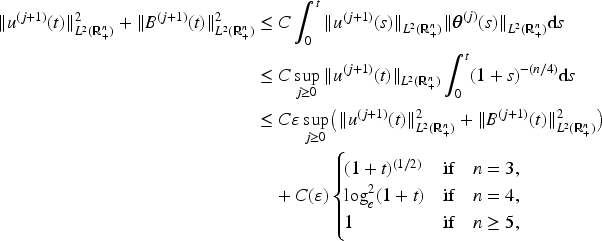
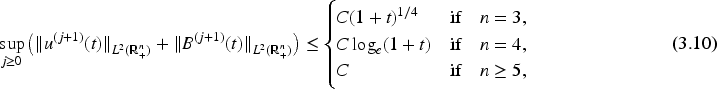
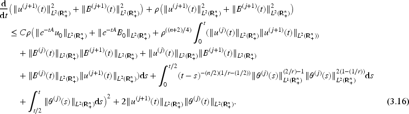
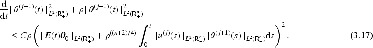
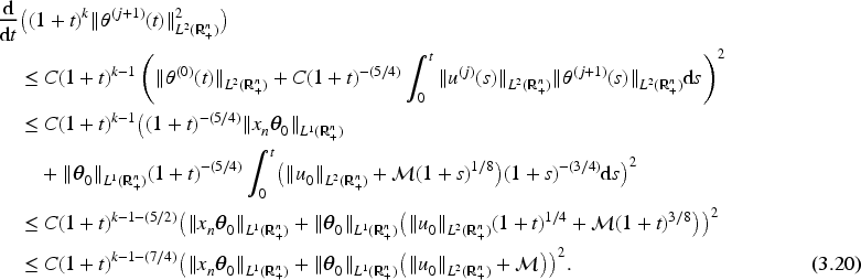
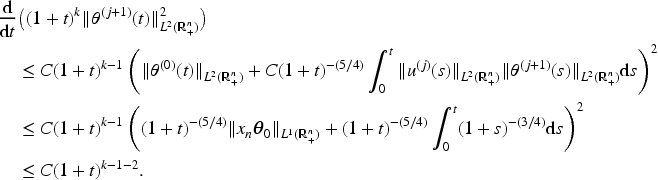
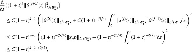
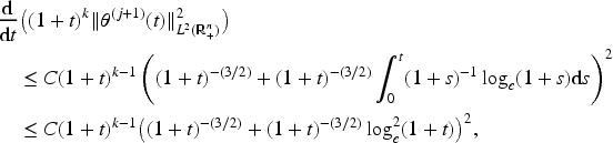
Set $ρ = k (1 + t)^{- 1},$ multiplying (3.17) by $(1 + t)^{k}$ , we combine the resulting expression with (3.7), (3.18), and (3.19) for $t > 0, j = 1, 2, \dots$

\begin{aligned} \frac{d}{d t} ((1 + t)^{k} ‖ θ^{(j + 1)} (t) ‖_{L^{2} (R_{+}^{n})}^{2}) \\ \leq C (1 + t)^{k - 1} {(‖ θ^{(0)} (t) ‖_{L^{2} (R_{+}^{n})} + C (1 + t)^{- (5 / 4)} \int_{0}^{t} ‖ u^{(j)} (s) ‖_{L^{2} (R_{+}^{n})} ‖ θ^{(j + 1)} (s) ‖_{L^{2} (R_{+}^{n})} d s)}^{2} \\ \leq C (1 + t)^{k - 1} ((1 + t)^{- (5 / 4)} ‖ x_{n} θ_{0} ‖_{L^{1} (R_{+}^{n})} \\ + ‖ θ_{0} ‖_{L^{1} (R_{+}^{n})} (1 + t)^{- (5 / 4)} \int_{0}^{t} (‖ u_{0} ‖_{L^{2} (R_{+}^{n})} + M (1 + s)^{1 / 8}) (1 + s)^{- (3 / 4)} d s)^{2} \\ \leq C (1 + t)^{k - 1 - (5 / 2)} (‖ x_{n} θ_{0} ‖_{L^{1} (R_{+}^{n})} + ‖ θ_{0} ‖_{L^{1} (R_{+}^{n})} (‖ u_{0} ‖_{L^{2} (R_{+}^{n})} (1 + t)^{1 / 4} + M (1 + t)^{3 / 8}))^{2} \\ \leq C (1 + t)^{k - 1 - (7 / 4)} (‖ x_{n} θ_{0} ‖_{L^{1} (R_{+}^{n})} + ‖ θ_{0} ‖_{L^{1} (R_{+}^{n})} (‖ u_{0} ‖_{L^{2} (R_{+}^{n})} + M))^{2} . \end{aligned}

(3.20)

Let

k > 0

be taken sufficiently large in (3.20), we infer for

t > 0

\begin{aligned} ‖ θ^{(j + 1)} (t) ‖_{L^{2} (R_{+}^{n})} \leq C ({‖ θ_{0} ‖}_{L^{2} (R_{+}^{n})} + {‖ x_{n} θ_{0} ‖}_{L^{1} (R_{+}^{n})} + {‖ θ_{0} ‖}_{L^{1} (R_{+}^{n})} ({‖ u_{0} ‖}_{L^{2} (R_{+}^{n})} + M)) (1 + t)^{- (7 / 8)} . \end{aligned}

(3.21)

Note that

‖ θ^{(0)} (t) ‖_{L^{2} (R_{+}^{n})} \leq C {‖ θ_{0} ‖}_{L^{1} (R_{+}^{n})} (1 + t)^{- (n / 4)} \leq C {‖ u_{0} ‖}_{L^{2} (R_{+}^{n})}

, by choosing

δ > 0

suitably small with

{‖ θ_{0} ‖}_{L^{1} (R_{+}^{n})} \leq δ

. From the above derivation process, it can be obtained

\begin{aligned} sup_{j \geq 0} ‖ θ^{(j)} (t) ‖_{L^{2} (R_{+}^{n})} \leq C (1 + t)^{- (7 / 8)} . \end{aligned}

(3.22)

By integrating (3.19) and (3.22), using the procedure from (3.21), yields for all

j \geq 0, t > 0

\begin{aligned} \frac{d}{d t} ((1 + t)^{k} ‖ θ^{(j + 1)} (t) ‖_{L^{2} (R_{+}^{n})}^{2}) \\ \leq C (1 + t)^{k - 1} {(‖ θ^{(0)} (t) ‖_{L^{2} (R_{+}^{n})} + C (1 + t)^{- (5 / 4)} \int_{0}^{t} ‖ u^{(j)} (s) ‖_{L^{2} (R_{+}^{n})} ‖ θ^{(j + 1)} (s) ‖_{L^{2} (R_{+}^{n})} d s)}^{2} \\ \leq C (1 + t)^{k - 1} {((1 + t)^{- (5 / 4)} ‖ x_{n} θ_{0} ‖_{L^{1} (R_{+}^{n})} + (1 + t)^{- (5 / 4)} \int_{0}^{t} (1 + s)^{- (3 / 4)} d s)}^{2} \\ \leq C (1 + t)^{k - 1 - 2} . \end{aligned}

Thus, it follows that

sup_{j \geq 0} ‖ θ^{(j)} (t) ‖_{L^{2} (R_{+}^{n})} \leq C (1 + t)^{- 1}

for

k

suitably large and

t > 0

. Combining (3.19) and still repeat the proof process of (3.21), we have

\begin{aligned} \frac{d}{d t} ((1 + t)^{k} ‖ θ^{(j + 1)} (t) ‖_{L^{2} (R_{+}^{n})}^{2}) \\ \leq C (1 + t)^{k - 1} {(‖ θ^{(0)} (t) ‖_{L^{2} (R_{+}^{n})} + C (1 + t)^{- (5 / 4)} \int_{0}^{t} ‖ u^{(j)} (s) ‖_{L^{2} (R_{+}^{n})} ‖ θ^{(j + 1)} (s) ‖_{L^{2} (R_{+}^{n})} d s)}^{2} \\ \leq C (1 + t)^{k - 1} {((1 + t)^{- (5 / 4)} ‖ x_{n} θ_{0} ‖_{L^{1} (R_{+}^{n})} + (1 + t)^{- (5 / 4)} \int_{0}^{t} (1 + s)^{- (7 / 8)} d s)}^{2} \\ \leq C (1 + t)^{k - 1 - (9 / 4)}, \end{aligned}

from which,

sup_{j \geq 0} ‖ θ^{(j)} (t) ‖_{L^{2} (R_{+}^{n})} \leq C (1 + t)^{- (9 / 8)}

. This inequality combined with (3.8) gives

\begin{aligned} sup_{j \geq 0} (‖ u^{(j)} (t) ‖_{L^{2} (R_{+}^{n})} + ‖ B^{(j)} (t) ‖_{L^{2} (R_{+}^{n})}) \leq C . \end{aligned}

(3.23)

Thus, by employing the new bounds on

‖ θ^{(j)} (t) ‖_{L^{2} (R_{+}^{n})}

and

sup_{j \geq 0} ‖ u^{(j)} (t) ‖_{L^{2} (R_{+}^{n})}

, following the procedure used to obtain (3.21), we get for

t > 0

\begin{aligned} \frac{d}{d t} ((1 + t)^{k} ‖ θ^{(j + 1)} (t) ‖_{L^{2} (R_{+}^{n})}^{2}) \\ \leq C (1 + t)^{k - 1} {(‖ θ^{(0)} (t) ‖_{L^{2} (R_{+}^{n})} + C (1 + t)^{- (5 / 4)} \int_{0}^{t} ‖ u^{(j)} (s) ‖_{L^{2} (R_{+}^{n})} ‖ θ^{(j + 1)} (s) ‖_{L^{2} (R_{+}^{n})} d s)}^{2} \\ \leq C (1 + t)^{k - 1} {((1 + t)^{- (5 / 4)} ‖ x_{n} b ‖_{L^{1} (R_{+}^{n})} + (1 + t)^{- (5 / 4)} \int_{0}^{t} (1 + s)^{- (9 / 8)} d s)}^{2} \\ \leq C (1 + t)^{k - 1 - (5 / 2)}, \end{aligned}

which implies that

\begin{aligned} sup_{j \geq 0} ‖ θ^{(j)} (t) ‖_{L^{2} (R_{+}^{n})} \leq C (1 + t)^{- (5 / 4)} . \end{aligned}

(3.24)

We finish the proof when

n = 3

. □

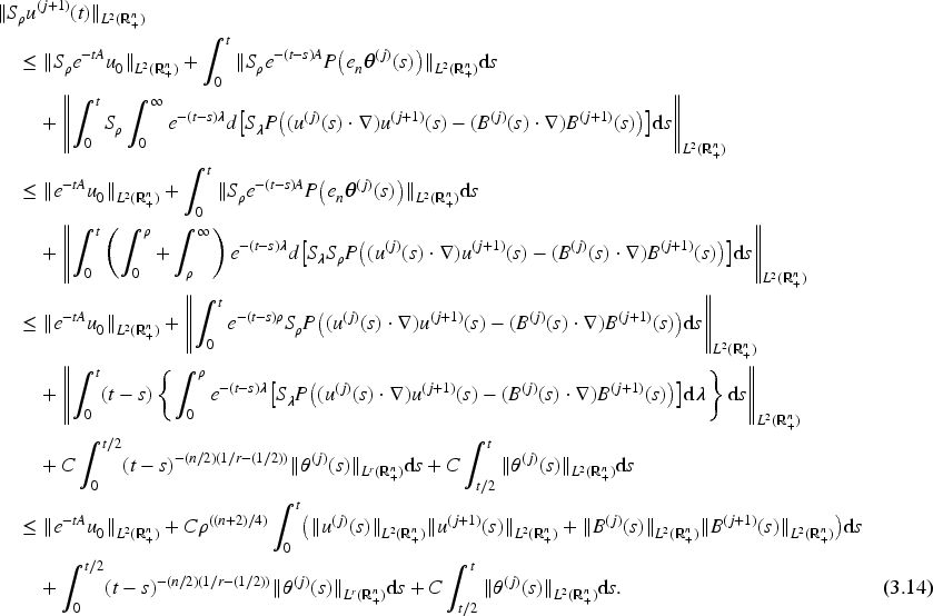
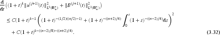
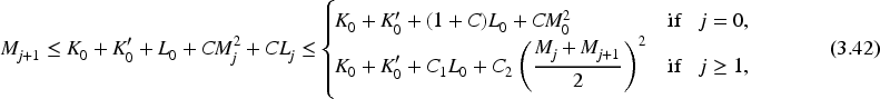
Case $n = 4$ . Setting $ρ = k (1 + t)^{- 1}$ where $k$ is a sufficiently large positive integer, we multiply both sides of (3.14) by $(1 + t)^{k}$ , together with (3.18) and (3.20), yields any $t > 0 and j = 0, 1, 2, \dots$

\begin{aligned} \frac{d}{d t} ((1 + t)^{k} ‖ θ^{(j + 1)} (t) ‖_{L^{2} (R_{+}^{n})}^{2}) \\ \leq C (1 + t)^{k - 1} {((1 + t)^{- (3 / 2)} + (1 + t)^{- (3 / 2)} \int_{0}^{t} (1 + s)^{- 1} \log_{e} (1 + s) d s)}^{2} \\ \leq C (1 + t)^{k - 1} ((1 + t)^{- (3 / 2)} + (1 + t)^{- (3 / 2)} \log_{e}^{2} (1 + t))^{2}, \end{aligned}

which implies for any

t > 0

sup_{j \geq 0} ‖ θ^{(j + 1)} (t) ‖_{L^{2} (R_{+}^{n})} \leq C (1 + t)^{- (3 / 2)} \log_{e}^{2} (1 + t) .

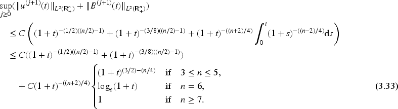
Repeating the process above, the new estimate implies that for

t > 0

and

j = 0, 1, 2, \dots

\begin{aligned} \frac{d}{d t} ((1 + t)^{k} ‖ θ^{(j + 1)} (t) ‖_{L^{2} (R_{+}^{n})}^{2}) \\ \leq C (1 + t)^{k - 1} {((1 + t)^{- (3 / 2)} + (1 + t)^{- (3 / 2)} \int_{0}^{t} (1 + s)^{- 1} \log_{e}^{3} (1 + s) d s)}^{2} \\ \leq C (1 + t)^{k - 4}, \end{aligned}

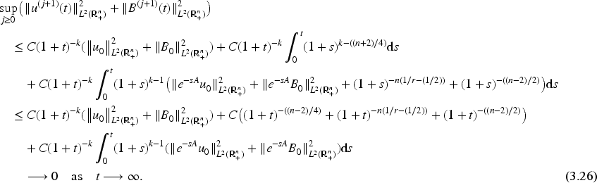
from which, we deduce that

sup_{j \geq 0} ‖ θ^{(j + 1)} (t) ‖_{L^{2} (R_{+}^{n})} \leq C (1 + t)^{- (3 / 2)} .

This shows the case

n = 4

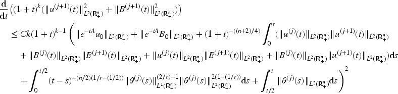
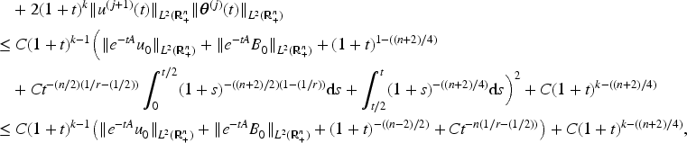
Case $n \geq 5$ . In this case, by repeating the proof process for the case $n = 4$ and using (3.10), it can be verified that (3.23) and (3.24) still hold true. Based on the above arguments, we have established that for $n \geq 3$ ,

\begin{aligned} sup_{j \geq 0} ‖ θ^{(j + 1)} (t) ‖_{L^{2} (R_{+}^{n})} \leq C (1 + t)^{- ((n + 2) / 4)} . \end{aligned}

(3.25)

In what follows, we prove (1.6). As we have noted (see Borchers & Miyakawa, 1988)

‖ e^{- t A} u_{0} ‖_{L^{2} (R_{+}^{n})} ⟶ 0, ‖ e^{- t A} B_{0} ‖_{L^{2} (R_{+}^{n})} ⟶ 0 as t ⟶ \infty,

which combines Lemma 2.6 and implies that

sup_{j \geq 0} ‖ θ^{(j)} (t) ‖_{L^{1} (R_{+}^{n})} \leq C .

Multiply both sides of (3.16) by

(1 + t)^{k}

and set

ρ = k (1 + t)^{- 1}

with

k > 1

, then combining (3.23) and (3.25), integrating over the interval

[0, t]

, we obtain for

t > 0

\begin{aligned} \frac{d}{d t} ((1 + t)^{k} (‖ u^{(j + 1)} (t) ‖_{L^{2} (R_{+}^{n})}^{2} + ‖ B^{(j + 1)} (t) ‖_{L^{2} (R_{+}^{n})}^{2})) \\ \leq C k (1 + t)^{k - 1} (‖ e^{- t A} u_{0} ‖_{L^{2} (R_{+}^{n})} + ‖ e^{- t A} B_{0} ‖_{L^{2} (R_{+}^{n})} + (1 + t)^{- ((n + 2) / 4)} \int_{0}^{t} (‖ u^{(j)} (t) ‖_{L^{2} (R_{+}^{n})} ‖ u^{(j + 1)} (t) ‖_{L^{2} (R_{+}^{n})} \\ + ‖ B^{(j)} (t) ‖_{L^{2} (R_{+}^{n})} ‖ B^{(j + 1)} (t) ‖_{L^{2} (R_{+}^{n})} + ‖ u^{(j)} (t) ‖_{L^{2} (R_{+}^{n})} ‖ B^{(j + 1)} (t) ‖_{L^{2} (R_{+}^{n})} + ‖ B^{(j)} (t) ‖_{L^{2} (R_{+}^{n})} ‖ u^{(j + 1)} (t) ‖_{L^{2} (R_{+}^{n})}) d s \\ {+ \int_{0}^{t / 2} (t - s)^{- (n / 2) (1 / r - (1 / 2))} ‖ θ^{(j)} (s) ‖_{L^{1} (R_{+}^{n})}^{(2 / r) - 1} ‖ θ^{(j)} (s) ‖_{L^{2} (R_{+}^{n})}^{2 (1 - (1 / r))} d s + \int_{t / 2}^{t} ‖ θ^{(j)} (s) ‖_{L^{2} (R_{+}^{n})} d s)}^{2} \\ + 2 (1 + t)^{k} ‖ u^{(j + 1)} (t) ‖_{L^{2} (R_{+}^{n}} ‖ θ^{(j)} (t) ‖_{L^{2} (R_{+}^{n})} \\ \leq C (1 + t)^{k - 1} (‖ e^{- t A} u_{0} ‖_{L^{2} (R_{+}^{n})} + ‖ e^{- t A} B_{0} ‖_{L^{2} (R_{+}^{n})} + (1 + t)^{1 - ((n + 2) / 4)} \\ + C t^{- (n / 2) (1 / r - (1 / 2))} \int_{0}^{t / 2} (1 + s)^{- ((n + 2) / 2) (1 - (1 / r))} d s + \int_{t / 2}^{t} (1 + s)^{- ((n + 2) / 4)} d s)^{2} + C (1 + t)^{k - ((n + 2) / 4)} \\ \leq C (1 + t)^{k - 1} (‖ e^{- t A} u_{0} ‖_{L^{2} (R_{+}^{n})} + ‖ e^{- t A} B_{0} ‖_{L^{2} (R_{+}^{n})} + (1 + t)^{- ((n - 2) / 2)} + C t^{- n (1 / r - (1 / 2))}) + C (1 + t)^{k - ((n + 2) / 4)}, \end{aligned}

where we choose

(n + 2) / 2 < r < 2

to ensure

\int_{0}^{t / 2} (1 + s)^{- ((n + 2) / 2) (1 - (1 / r))} < \infty

, then

\begin{aligned} sup_{j \geq 0} (‖ u^{(j + 1)} (t) ‖_{L^{2} (R_{+}^{n})}^{2} + ‖ B^{(j + 1)} (t) ‖_{L^{2} (R_{+}^{n})}^{2}) \\ \leq C (1 + t)^{- k} ({‖ u_{0} ‖}_{L^{2} (R_{+}^{n})}^{2} + ‖ B_{0} ‖_{L^{2} (R_{+}^{n})}^{2}) + C (1 + t)^{- k} \int_{0}^{t} (1 + s)^{k - ((n + 2) / 4)} d s \\ + C (1 + t)^{- k} \int_{0}^{t} (1 + s)^{k - 1} (‖ e^{- s A} u_{0} ‖_{L^{2} (R_{+}^{n})}^{2} + ‖ e^{- s A} B_{0} ‖_{L^{2} (R_{+}^{n})}^{2} + (1 + s)^{- n (1 / r - (1 / 2))} + (1 + s)^{- ((n - 2) / 2)}) d s \\ \leq C (1 + t)^{- k} ({‖ u_{0} ‖}_{L^{2} (R_{+}^{n})}^{2} + ‖ B_{0} ‖_{L^{2} (R_{+}^{n})}^{2}) + C ((1 + t)^{- ((n - 2) / 4)} + (1 + t)^{- n (1 / r - (1 / 2))} + (1 + t)^{- ((n - 2) / 2)}) \\ + C (1 + t)^{- k} \int_{0}^{t} (1 + s)^{k - 1} (‖ e^{- s A} u_{0} ‖_{L^{2} (R_{+}^{n})}^{2} + ‖ e^{- s A} B_{0} ‖_{L^{2} (R_{+}^{n})}^{2}) d s \\ ⟶ 0 as t ⟶ \infty . \end{aligned}

(3.26)

This completes the proof of the second part of the theorem. □

To prove (1.7), we assume that $u_{0}, B_{0} \in L^{(n / (n - 1))} (R_{+}^{n})$ . First, we require two auxiliary estimates to proceed, specifically, we derive the bounds for $‖ θ^{(j + 1)} ‖_{L^{1} (R_{+}^{n})}$ , $‖ u^{(j + 1)} ‖_{L^{2} (R_{+}^{n})}$ , and $‖ B^{(j + 1)} ‖_{L^{2} (R_{+}^{n})}$ as follows.

By (3.1), combining (3.23) and (3.25), it follows that

\begin{aligned} ‖ θ^{(j + 1)} (t) ‖_{L^{1} (R_{+}^{n})} & \leq ‖ E (t) θ_{0} ‖_{L^{1} (R_{+}^{n})} + C \int_{0}^{t} {‖ \nabla G_{t - s} ‖}_{L^{1} (R_{+}^{n})} ‖ u^{(j)} (s) θ^{(j + 1)} (s) ‖_{L^{1} (R_{+}^{n})} d s \\ \leq C t^{- (1 / 2)} {‖ x_{n} θ_{0} ‖}_{L^{1} (R_{+}^{n})} + C \int_{0}^{t} (t - s)^{- (1 / 2)} ‖ u^{(j)} (s) ‖_{L^{2} (R_{+}^{n})} ‖ θ^{(j + 1)} (s) ‖_{L^{2} (R_{+}^{n})} d s \\ \leq C t^{- (1 / 2)} + C (\int_{0}^{t / 2} + \int_{t / 2}^{t}) (t - s)^{- (1 / 2)} (1 + s)^{- ((n + 2) / 4)} d s \\ \leq C t^{- (1 / 2)} + C (1 + t)^{- (n / 4)} \\ \leq C (1 + t)^{- (1 / 2)} . \end{aligned}

(3.27)

Setting

1 < r < 2

, we obtain for

t > 0 and j = 0, 1, 2, \dots

\begin{aligned} \int_{0}^{t / 2} (t - s)^{- (n / 2) (1 / r - (1 / 2))} ‖ θ^{(j)} (s) ‖_{L^{1} (R_{+}^{n})}^{(2 / r) - 1} ‖ θ^{(j)} (s) ‖_{L^{2} (R_{+}^{n})}^{2 (1 - (1 / r))} d s + \int_{t / 2}^{t} ‖ θ^{(j)} (s) ‖_{L^{2} (R_{+}^{n})} d s \\ \leq C t^{- (n / 2) (1 / r - (1 / 2))} \int_{0}^{t / 2} (1 + s)^{- (1 / 2) ((2 / r) - 1) - ((n + 2) / 2) (1 - (1 / r))} d s + C \int_{t / 2}^{t} (1 + s)^{- ((n + 2) / 4)} d s \\ \leq C (1 + t)^{- (1 / 2) (2 / n - 1)} . \end{aligned}

(3.28)

By Lemma 2.4, (3.25) and (3.28), we have for $t > 0 and j = 0, 1, 2, \dots$

\begin{aligned} \frac{d}{d t} (‖ u^{(j + 1)} (t) ‖_{L^{2} (R_{+}^{n})}^{2} + ‖ B^{(j + 1)} (t) ‖_{L^{2} (R_{+}^{n})}^{2}) + ρ (‖ u^{(j + 1)} (t) ‖_{L^{2} (R_{+}^{n})}^{2} + ‖ B^{(j + 1)} (t) ‖_{L^{2} (R_{+}^{n})}^{2}) \\ \leq C ρ ((1 + t)^{- (1 / 2) ((n / 2) - 1)} (1 + {‖ u_{0} ‖}_{L^{(n / (n - 1))} (R_{+}^{n})} + {‖ B_{0} ‖}_{L^{(n / (n - 1))} (R_{+}^{n})}) \\ + ρ^{(n + 2) / 4} \int_{0}^{t} (‖ u^{(j)} (t) ‖_{L^{2} (R_{+}^{n})} ‖ u^{(j + 1)} (t) ‖_{L^{2} (R_{+}^{n})} + ‖ B^{(j)} (t) ‖_{L^{2} (R_{+}^{n})} ‖ B^{(j + 1)} (t) ‖_{L^{2} (R_{+}^{n})} \\ + ‖ u^{(j)} (t) ‖_{L^{2} (R_{+}^{n})} ‖ B^{(j + 1)} (t) ‖_{L^{2} (R_{+}^{n})} + ‖ B^{(j)} (t) ‖_{L^{2} (R_{+}^{n})} ‖ u^{(j + 1)} (t) ‖_{L^{2} (R_{+}^{n})}) d s)^{2} \\ + C ‖ u^{(j + 1)} (t) ‖_{L^{2} (R_{+}^{n})} (1 + t)^{- ((n + 2) / 4)} . \end{aligned}

(3.29)

Let

ρ

be defined as before, by employing the method used previously and applying (3.23), we obtain

\begin{aligned} \frac{d}{d t} ((1 + t)^{k} (‖ u^{(j + 1)} (t) ‖_{L^{2} (R_{+}^{n})}^{2} + ‖ B^{(j + 1)} (t) ‖_{L^{2} (R_{+}^{n})}^{2})) \leq C (1 + t)^{k - 1 - ((n / 2) - 1)} + C (1 + t)^{k - ((n + 2) / 4)} . \end{aligned}

(3.30)

Integrating both sides of the above inequality yields

\begin{aligned} sup_{j \geq 0} (‖ u^{(j + 1)} (t) ‖_{L^{2} (R_{+}^{n})} + ‖ B^{(j + 1)} (t) ‖_{L^{2} (R_{+}^{n})}) \leq C (1 + t)^{- ((n - 2) / 8)} . \end{aligned}

(3.31)

We now use the new estimate (3.31) and repeat the steps leading to (3.30), we obtain for any

t > 0 and j = 0, 1, 2, \dots

\begin{aligned} \frac{d}{d t} ((1 + t)^{k} ‖ u^{(j + 1)} (t) ‖_{L^{2} (R_{+}^{n})}^{2} + ‖ B^{(j + 1)} (t) ‖_{L^{2} (R_{+}^{n})}^{2}) \\ \leq C (1 + t)^{k - 1} {((1 + t)^{- (1 / 2) ((n / 2) - 1)} + (1 + t)^{- ((n + 2) / 4)} \int_{0}^{t} (1 + s)^{- ((n - 2) / 4)} d s)}^{2} \\ + C (1 + t)^{k - ((n - 2) / 8) - ((n + 2) / 4)} . \end{aligned}

(3.32)

Integrating (3.32) gives

\begin{aligned} sup_{j \geq 0} (‖ u^{(j + 1)} (t) ‖_{L^{2} (R_{+}^{n})} + ‖ B^{(j + 1)} (t) ‖_{L^{2} (R_{+}^{n})}) \\ \leq C ((1 + t)^{- (1 / 2) ((n / 2) - 1)} + (1 + t)^{- (3 / 8) ((n / 2) - 1)} + (1 + t)^{- ((n + 2) / 4)} \int_{0}^{t} (1 + s)^{- ((n - 2) / 4)} d s) \\ \leq C ((1 + t)^{- (1 / 2) ((n / 2) - 1)} + (1 + t)^{- (3 / 8) ((n / 2) - 1)}) \\ + C (1 + t)^{- ((n + 2) / 4)} {\begin{cases} (1 + t)^{(3 / 2) - (n / 4)} & if 3 \leq n \leq 5, \\ \log_{e} (1 + t) & if n = 6, \\ 1 & if n \geq 7. \end{cases} \end{aligned}

(3.33)

We replicate the steps used to derive (3.33) and thereby obtain

\begin{aligned} sup_{j \geq 0} (‖ u^{(j + 1)} (t) ‖_{L^{2} (R_{+}^{n})} + ‖ B^{(j + 1)} (t) ‖_{L^{2} (R_{+}^{n})}) \leq C_{m} ((1 + t)^{- (1 / 2) ((n / 2) - 1)} + (1 + t)^{- ((m - 1) / m) ((1 / 2) ((n / 2) - 1))}) . \end{aligned}

(3.34)

Then, for any small

ϵ > 0

, there exists a sufficiently large

m_{0} = m_{0} (ϵ) > 0

satisfying

\begin{aligned} sup_{j \geq 0} (‖ u^{(j + 1)} (t) ‖_{L^{2} (R_{+}^{n})} + ‖ B^{(j + 1)} (t) ‖_{L^{2} (R_{+}^{n})}) \leq C_{m_{0}} (1 + t)^{- ((n - 2) / 4) + ϵ} . \end{aligned}

(3.35)

Furthermore, we can find

\begin{aligned} ‖ u^{(j)} ‖_{L^{\infty} (0, \infty; L^{2} (R_{+}^{n}))} + ‖ \nabla u^{(j)} ‖_{L^{2} (0, \infty; L^{2} (R_{+}^{n}))} \leq C, \\ ‖ B^{(j)} ‖_{L^{\infty} (0, \infty; L^{2} (R_{+}^{n}))} + ‖ \nabla B^{(j)} ‖_{L^{2} (0, \infty; L^{2} (R_{+}^{n}))} \leq C, \\ ‖ θ^{(j)} ‖_{L^{\infty} (0, \infty; L^{2} (R_{+}^{n}))} + ‖ \nabla θ^{(j)} ‖_{L^{2} (0, \infty; L^{2} (R_{+}^{n}))} \leq C . \end{aligned}

Using the Banach–Alaoglu Theorem and Aubin–Lions Lemma, it is possible to find a subsequence

(u^{(j)}, B^{(j)}, θ^{(j)})

(u, B, θ)

such that as

j ⟶ \infty

\begin{aligned} u^{(j)} \overset{*}{⇀} u weakly in L^{\infty} (0, \infty; L^{2} (R_{+}^{n})), \nabla u^{(j)} ⇀ \nabla u weakly in L^{2} (0, \infty; L^{2} (R_{+}^{n})); \\ B^{(j)} \overset{*}{⇀} B weakly in L^{\infty} (0, \infty; L^{2} (R_{+}^{n})), \nabla B^{(j)} ⇀ \nabla B weakly in L^{2} (0, \infty; L^{2} (R_{+}^{n})); \\ θ^{(j)} \overset{*}{⇀} θ weakly in L^{\infty} (0, \infty; L^{2} (R_{+}^{n})), \nabla θ^{(j)} ⇀ \nabla θ weakly in L^{2} (0, \infty; L^{2} (R_{+}^{n})) . \end{aligned}

It follows that $u, B \in L^{\infty} (0, T; L_{σ}^{2} (R_{+}^{n})) \cap L^{2} (0, T; H_{0}^{1} (R_{+}^{n})) and θ \in L^{\infty} (0, T; L^{2} (R_{+}^{n})) \cap L^{2} (0, T; H_{0}^{1} (R_{+}^{n}))$ for all $t > 0$ . Therefore, $(u, B, θ)$ is a weak solution to problem (1.1) as claimed.

We thus finish the proof of Theorem 1.1. □

3.2.

L^{q}

-Decay of Strong Solutions

The main goal of this subsection is to establish $L^{q}$ -decay of strong solutions to problem (1.1).

Proof of Theorem 1.2. Inspired by Kato’s thought, we consider the corresponding approximate problem for $j = 0, 1, 2 \dots$

\begin{aligned} {\begin{aligned} θ^{(0)} (t) = E (t) θ_{0}, u^{(0)} (t) = e^{- t A} u_{0}, B^{(0)} (t) = e^{- t A} B_{0}, \\ θ^{(j + 1)} (t) = θ^{(0)} (t) - \int_{0}^{t} E (t - s) u^{(j)} (s) \cdot θ^{(j)} (s) d s, \\ u^{(j + 1)} (t) = u^{(0)} (t) - \int_{0}^{t} e^{- (t - s) A} P (u^{(j)} (s) \cdot \nabla u^{(j)} (s) - B^{(j)} (s) \cdot \nabla B^{(j)} (s) - θ^{(j)} (s) e_{n}) d s, \\ B^{(j + 1)} (t) = B^{(0)} (t) - \int_{0}^{t} e^{- (t - s) A} P (u^{(j)} (s) \cdot \nabla B^{(j)} (s) - B^{(j)} (s) \cdot \nabla u^{(j)} (s)) d s . \end{aligned} \end{aligned}

(3.36)

First, we estimate $‖ u^{(j + 1)} (t) ‖_{L^{n / δ} (R_{+}^{n})}$ , $‖ B^{(j + 1)} (t) ‖_{L^{n / δ} (R_{+}^{n})}$ and $‖ θ^{(j + 1)} (t) ‖_{L^{n / α} (R_{+}^{n})}$ respectively through induction and iteration, which is crucial for the following proof. Let $1 < α < 2$ and $0 < δ < 1$ , we define for $j = 0, 1, 2 \dots$

\begin{aligned} K_{j} = sup_{0 < t < \infty} (t^{(1 - δ) / 2} (‖ u^{(j)} (t) ‖_{L^{n / δ}} + ‖ B^{(j)} (t) ‖_{L^{n / δ}})), \\ K_{j}^{'} = sup_{0 < t < \infty} (t^{(1 / 2)} (‖ \nabla u^{(j)} (t) ‖_{L^{n}} + ‖ \nabla B^{(j)} (t) ‖_{L^{n}})) \end{aligned}

and

L_{j} = sup_{0 < t < \infty} (t^{(3 - α) / 2} ‖ θ^{(j)} (t) ‖_{L^{n / α}}) .

Using Lemma 2.4, we have

\begin{aligned} {‖ u^{(0)} (t) ‖}_{L^{n / δ} (R_{+}^{n})} + {‖ B^{(0)} (t) ‖}_{L^{n / δ} (R_{+}^{n})} \leq C t^{- ((1 - δ) / 2)} ({‖ u_{0} ‖}_{L^{n} (R_{+}^{n})} + {‖ B_{0} ‖}_{L^{n} (R_{+}^{n})}), \\ {‖ \nabla u^{(0)} (t) ‖}_{L^{n / δ} (R_{+}^{n})} + {‖ \nabla B^{(0)} (t) ‖}_{L^{n / δ} (R_{+}^{n})} \leq C t^{- (1 / 2)} ({‖ u_{0} ‖}_{L^{n} (R_{+}^{n})} + {‖ B_{0} ‖}_{L^{n} (R_{+}^{n})}) \end{aligned}

and

{‖ θ^{(0)} (t) ‖}_{L^{n / α} (R_{+}^{n})} = ‖ E (t) θ_{0} ‖_{L^{n / α} (R_{+}^{n})} \leq C t^{- ((3 - α) / 2)} {‖ θ_{0} ‖}_{L^{n} (R_{+}^{n})} .

Thus, we have $K_{0} + K_{0}^{'} + L_{0} \leq C {‖ u_{0} ‖}_{L^{n} (R_{+}^{n})} + C {‖ B_{0} ‖}_{L^{n} (R_{+}^{n})} + C {‖ θ_{0} ‖}_{L^{n} / 3 (R_{+}^{n})} < \infty$ . Now, we assume $K_{j} + K_{j}^{'} + L_{j} < \infty$ , from Lemma 2.4, we have for $t > 0$

\begin{aligned} ‖ u^{(j + 1)} (t) ‖_{L^{n / δ} (R_{+}^{n})} + ‖ B^{(j + 1)} (t) ‖_{L^{n / δ} (R_{+}^{n})} \\ \leq ‖ e^{- t A} u_{0} ‖_{L^{n / δ} (R_{+}^{n})} + \int_{0}^{t} ‖ e^{- (t - s) A} P (u^{(j)} (s) \cdot \nabla u^{(j)} (s) - B^{(j)} (s) \cdot \nabla B^{(j)} (s) - θ^{(j)} (s) e_{n}) ‖_{L^{n / δ} (R_{+}^{n})} d s \\ + ‖ e^{- t A} B_{0} ‖_{L^{n / δ} (R_{+}^{n})} + \int_{0}^{t} ‖ e^{- (t - s) A} P (u^{(j)} (s) \cdot \nabla B^{(j)} (s) - B^{(j)} (s) \cdot \nabla u^{(j)} (s)) ‖_{L^{n / δ} (R_{+}^{n})} d s \\ \leq K_{0} t^{- ((1 - δ) / 2)} + C \int_{0}^{t} (t - s)^{- (1 / 2)} (‖ u^{(j)} (s) ‖_{L^{n / δ} (R_{+}^{n})} ‖ \nabla u^{(j)} (s) ‖_{L^{n} (R_{+}^{n})} + ‖ B^{(j)} (s) ‖_{L^{n / δ} (R_{+}^{n})} ‖ \nabla B^{(j)} (s) ‖_{L^{n} (R_{+}^{n})} \\ + ‖ u^{(j)} (s) ‖_{L^{n / δ} (R_{+}^{n})} ‖ \nabla B^{(j)} (s) ‖_{L^{n} (R_{+}^{n})} + ‖ B^{(j)} (s) ‖_{L^{n / δ} (R_{+}^{n})} ‖ \nabla u^{(j)} (s) ‖_{L^{n} (R_{+}^{n})}) d s \\ + C \int_{0}^{t} (t - s)^{- (n / 2) ((α / n) - (δ / n))} ‖ θ^{(j)} (s) ‖_{L^{n / α} (R_{+}^{n})} d s \\ \leq K_{0} t^{- ((1 - δ) / 2)} + C K_{j} K_{j}^{'} \int_{0}^{t} (t - s)^{- (1 / 2)} s^{- 1 + (δ / 2)} d s + C L_{j} \int_{0}^{t} (t - s)^{- ((α - δ) / 2)} s^{- ((3 - α) / 2)} d s \\ \leq K_{0} t^{- ((1 - δ) / 2)} + C K_{j} K_{j}^{'} t^{- ((1 - δ) / 2)} + C L_{j} t^{- ((1 - δ) / 2)} . \end{aligned}

(3.37)

Hence

\begin{aligned} K_{j + 1} \leq K_{0} + C K_{j} K_{j}^{'} + C L_{j} < \infty . \end{aligned}

(3.38)

Similarly, it holds that

\begin{aligned} ‖ \nabla u^{(j + 1)} (t) ‖_{L^{n} (R_{+}^{n})} + ‖ \nabla B^{(j + 1)} (t) ‖_{L^{n} (R_{+}^{n})} \\ \leq ‖ \nabla e^{- t A} u_{0} ‖_{L^{n} (R_{+}^{n})} + \int_{0}^{t} ‖ \nabla e^{- (t - s) A} P (u^{(j)} (s) \cdot \nabla u^{(j)} (s) - B^{(j)} (s) \cdot \nabla B^{(j)} (s) - θ^{(j)} (s) e_{n}) ‖_{L^{n} (R_{+}^{n})} d s \\ + ‖ \nabla e^{- t A} B_{0} ‖_{L^{n} (R_{+}^{n})} + \int_{0}^{t} ‖ \nabla e^{- (t - s) A} P (u^{(j)} (s) \cdot \nabla B^{(j)} (s) - B^{(j)} (s) \cdot \nabla u^{(j)} (s)) ‖_{L^{n / δ} (R_{+}^{n})} d s \\ \leq K_{0}^{'} t^{- (1 / 2)} + C \int_{0}^{t} (t - s)^{- ((1 + δ) / 2)} (‖ u^{(j)} (s) ‖_{L^{n / δ} (R_{+}^{n})} ‖ \nabla u^{(j)} (s) ‖_{L^{n} (R_{+}^{n})} + ‖ B^{(j)} (s) ‖_{L^{n / δ} (R_{+}^{n})} ‖ \nabla B^{(j)} (s) ‖_{L^{n} (R_{+}^{n})} \\ + ‖ u^{(j)} (s) ‖_{L^{n / δ} (R_{+}^{n})} ‖ \nabla B^{(j)} (s) ‖_{L^{n} (R_{+}^{n})} + ‖ B^{(j)} (s) ‖_{L^{n / δ} (R_{+}^{n})} ‖ \nabla u^{(j)} (s) ‖_{L^{n} (R_{+}^{n})}) d s \\ + C \int_{0}^{t} (t - s)^{- (1 / 2) - (n / 2) (((α / n)) - (δ / n))} ‖ θ^{(j)} (s) ‖_{L^{n / α} (R_{+}^{n})} d s \\ \leq K_{0}^{'} t^{- (1 / 2)} + C K_{j} K_{j}^{'} \int_{0}^{t} (t - s)^{- ((1 + δ) / 2)} s^{- 1 + (δ / 2)} d s + C L_{j} \int_{0}^{t} (t - s)^{- (α / 2)} s^{- ((3 - α) / 2)} d s \\ \leq K_{0}^{'} t^{- (1 / 2)} + C K_{j} K_{j}^{'} t^{- (1 / 2)} + C L_{j} t^{- (1 / 2)}, \end{aligned}

which implies that

\begin{aligned} K_{j + 1}^{'} \leq K_{0}^{'} + C K_{j} K_{j}^{'} + C L_{j} < \infty . \end{aligned}

(3.39)

Likewise, with respect to

θ^{(j + 1)}

, we have

\begin{aligned} ‖ θ^{(j + 1)} (t) ‖_{L^{n / α}} \leq ‖ E (t) θ_{0} ‖_{L^{n / α} (R_{+}^{n})} + 2 \int_{0}^{t} ‖ \nabla G_{t - s} ‖_{L^{(1 - (δ / n))^{- 1}} (R^{n})} ‖ (u^{(j)} (s) θ^{(j)} (s)) ‖_{L^{n / (α + δ)} (R_{+}^{n})} d s \\ \leq L_{0} t^{- ((3 - α) / 2)} + C \int_{0}^{t} (t - s)^{- (1 / 2) - (δ / 2)} ‖ u^{(j)} (s) ‖_{L^{n / δ} (R_{+}^{n})} ‖ θ^{(j)} (s) ‖_{L^{n / α} (R_{+}^{n})} d s \\ \leq L_{0} t^{- ((3 - α) / 2)} + C K_{j} L_{j} \int_{0}^{t} (t - s)^{- ((1 + δ) / 2)} s^{- 2 + (α + δ) / 2} d s \\ \leq L_{0} t^{- ((3 - α) / 2)} + C K_{j} L_{j} t^{- ((3 - α) / 2)} . \end{aligned}

(3.40)

Thus

\begin{aligned} L_{j + 1} \leq L_{0} + C K_{j} L_{j} < \infty . \end{aligned}

(3.41)

Set $M_{j} = K_{j} + K_{j}^{'} + L_{j}$ for $j = 0, 1, 2 \dots$ . Based on the above estimates, we obtain from (3.38) to (3.41) that

\begin{aligned} M_{j + 1} \leq K_{0} + K_{0}^{'} + L_{0} + C M_{j}^{2} + C L_{j} \leq {\begin{cases} K_{0} + K_{0}^{'} + (1 + C) L_{0} + C M_{0}^{2} & if j = 0, \\ K_{0} + K_{0}^{'} + C_{1} L_{0} + C_{2} {(\frac{M_{j} + M_{j + 1}}{2})}^{2} & if j \geq 1, \end{cases} \end{aligned}

(3.42)

where

C_{1} > 1 + 2 C

C_{2} > 4 C

Let $Υ_{0} = K_{0} + K_{0}^{'} + C_{1} L_{0}$ . Note that $Υ_{0} \leq C ({‖ u_{0} ‖}_{L^{n} (R_{+}^{n})} + {‖ B_{0} ‖}_{L^{n} (R_{+}^{n})} + {‖ θ_{0} ‖}_{L^{n / 3} (R_{+}^{n})}) \leq C ϵ_{0}$ . Choosing $ϵ_{0}$ so small that $Υ_{0} < (1 / (4 C_{2}))$ and setting $X_{0} = (2 C_{2})^{- 1} (1 - \sqrt{1 - 4 Υ_{0} C_{2}})$ , We can obtain $X_{0} = B_{0} + C_{2} X_{0}^{2}$ and $X_{0} \leq 2 Υ_{0}$ . By induction, we can verify that

\begin{aligned} M_{j} \leq X_{0}, j = 0, 1, 2, \dots . \end{aligned}

(3.43)

Now, combining Lemma 2.4, (3.36), and (3.43) for

j = 0, 1, 2, \dots, t > 0

and

n \leq q \leq \infty

, we arrive at

\begin{aligned} ‖ u^{(j + 1)} (t) ‖_{L^{q} (R_{+}^{n})} + ‖ B^{(j + 1)} (t) ‖_{L^{q} (R_{+}^{n})} \\ \leq ‖ e^{- t A} u_{0} ‖_{L^{q} (R_{+}^{n})} + \int_{0}^{t} ‖ e^{- (t - s) A} P (u^{(j)} (s) \cdot \nabla u^{(j)} (s) - B^{(j)} (s) \cdot \nabla B^{(j)} (s) - θ^{(j)} (s) e_{n}) ‖_{L^{q} (R_{+}^{n})} d s \\ + ‖ e^{- t A} B_{0} ‖_{L^{q} (R_{+}^{n})} + \int_{0}^{t} ‖ e^{- (t - s) A} P (u^{(j)} (s) \cdot \nabla B^{(j)} (s) - B^{(j)} (s) \cdot \nabla u^{(j)} (s)) ‖_{L^{q} (R_{+}^{n})} d s \\ \leq C t^{- (n / 2) ((1 / n) - (1 / q))} ({‖ u_{0} ‖}_{L^{n} (R_{+}^{n})} + {‖ B_{0} ‖}_{L^{n} (R_{+}^{n})}) + C \int_{0}^{t} (t - s)^{- (n / 2) ((α / n) - (1 / q))} ‖ θ^{(j)} (s) ‖_{L^{n / α} (R_{+}^{n})} d s \\ + C \int_{0}^{t} (t - s)^{- (n / 2) (((1 + δ) / n) - (1 / q))} (‖ u^{(j)} (s) ‖_{L^{n / δ} (R_{+}^{n})} ‖ \nabla u^{(j)} (s) ‖_{L^{n} (R_{+}^{n})} + ‖ B^{(j)} (s) ‖_{L^{n / δ} (R_{+}^{n})} ‖ \nabla B^{(j)} (s) ‖_{L^{n} (R_{+}^{n})} \\ + ‖ u^{(j)} (s) ‖_{L^{n / δ} (R_{+}^{n})} ‖ \nabla B^{(j)} (s) ‖_{L^{n} (R_{+}^{n})} + ‖ B^{(j)} (s) ‖_{L^{n / δ} (R_{+}^{n})} ‖ \nabla u^{(j)} (s) ‖_{L^{n} (R_{+}^{n})}) d s \\ \leq C t^{- (n / 2) ((1 / n) - (1 / q))} ({‖ u_{0} ‖}_{L^{n} (R_{+}^{n})} + {‖ B_{0} ‖}_{L^{n} (R_{+}^{n})}) + C K_{j} K_{j}^{'} \int_{0}^{t} (t - s)^{- ((1 + δ) / 2) + (n / 2 q)} s^{- (1 + δ) / 2} d s \\ + C L_{j} \int_{0}^{t} (t - s)^{- (α / 2) + (n / 2 q)} s^{- ((3 - α) / 2)} d s \\ \leq C ({‖ u_{0} ‖}_{L^{n} (R_{+}^{n})} + {‖ B_{0} ‖}_{L^{n} (R_{+}^{n})} + M_{j} + M_{j}^{2}) t^{- (1 / 2) + (n / 2 q)} \\ \leq C ϵ_{0} t^{- (1 / 2) + (n / 2 q)} . \end{aligned}

(3.44)

Now, we estimate $‖ θ (t) ‖_{L^{q} (R_{+}^{n})}$ , it follows that for $j = 0, 1, 2, \dots$ and $t > 0$

\begin{aligned} θ^{(j + 1)} (t) = E (\frac{t}{2}) θ^{(j + 1)} (\frac{t}{2}) - \int_{t / 2}^{t} E (t - s) u^{(j)} (s) \cdot \nabla θ^{(j)} (s) d s . \end{aligned}

(3.45)

Set

n \leq q < \infty

, for sufficiently small

ϵ > 0

n \leq q < (n / (α - 1))

can be satisfied by choosing

α = 1 + 2 ϵ

. From Lemma 2.4 and (3.43)–(3.45), we derive that

\begin{aligned} ‖ θ^{(j + 1)} (t) ‖_{L^{q} (R_{+}^{n})} & \leq ‖ E (\frac{t}{2}) θ^{(j + 1)} (\frac{t}{2}) ‖_{L^{q} (R_{+}^{n})} \\ + 2 \int_{t / 2}^{t} ‖ \nabla G_{t - s} ‖_{L^{(1 + (1 / q) - ((α / n)))^{- 1}} (R^{n})} ‖ (u^{(j)} (s) θ^{(j)} (s)) ‖_{L^{n / α} (R_{+}^{n})} d s \\ \leq C t^{- (n / 2) ((α / n) - (1 / q))} ‖ θ^{(j + 1)} (\frac{t}{2}) ‖_{L^{n / α} (R_{+}^{n})} \\ + C \int_{t / 2}^{t} (t - s)^{- (1 / 2) - (n / 2) ((α / n) - (1 / q))} ‖ u^{(j)} (s) ‖_{L^{\infty} (R_{+}^{n})} ‖ θ^{(j)} (s) ‖_{L^{n / α} (R_{+}^{n})} d s \\ \leq C ϵ_{0} t^{- (n / 2) ((α / n) - (1 / q)) - ((3 - α) / 2)} + C ϵ_{0}^{2} \int_{t / 2}^{t} (t - s)^{- (1 / 2) - (n / 2) ((α / n) - (1 / q))} s^{- (1 / 2) - ((3 - α) / 2)} d s \\ \leq C ϵ_{0} t^{- (3 / 2) + (n / 2 q)} + C ϵ_{0}^{2} t^{- (1 / 2) - ((3 - α) / 2) + 1 - (1 / 2) - (n / 2) ((α / n) - (1 / q))} \\ \leq C ϵ_{0} t^{- (3 / 2) + (n / 2 q)} . \end{aligned}

(3.46)

Let

n \leq q \leq \infty

, setting

H_{j} (t) = sup_{0 < s \leq t} (s^{2 - (n / 2 q)} ‖ \nabla θ^{(j)} (t) ‖_{L^{q} (R_{+}^{n})})

, then we have

\begin{aligned} ‖ \nabla θ^{(j + 1)} (t) ‖_{L^{q} (R_{+}^{n})} \leq & ‖ \nabla E (\frac{t}{2}) θ^{(j + 1)} (\frac{t}{2}) ‖_{L^{q} (R_{+}^{n})} + \int_{t / 2}^{t} ‖ \nabla E (t - s) (u^{(j)} (s) \cdot \nabla θ^{(j)} (s)) ‖_{L^{q} (R_{+}^{n})} d s \\ \leq C t^{- (1 / 2)} ‖ θ^{(j + 1)} (t) ‖_{L^{q} (R_{+}^{n})} + C \int_{t / 2}^{t} (t - s)^{- (1 / 2)} ‖ u^{(j)} (s) ‖_{L^{\infty} (R_{+}^{n})} ‖ \nabla θ^{(j)} (s) ‖_{L^{q} (R_{+}^{n})} d s \\ \leq C ϵ_{0} t^{- 2 + (n / 2 q)} + C ϵ_{0} H_{j} (t) \int_{t / 2}^{t} (t - s)^{- (1 / 2)} s^{- (1 / 2) - 2 + (n / 2 q)} d s \\ \leq C ϵ_{0} t^{- 2 + (n / 2 q)} + C ϵ_{0} H_{j} (t) t^{- 2 + (n / 2 q)}, \end{aligned}

which implies that

\begin{aligned} H_{j + 1} (t) \leq C ϵ_{0} + C ϵ_{0} H_{j} (t) . \end{aligned}

(3.47)

Note that

‖ \nabla θ^{(0)} (s) ‖_{L^{q} (R_{+}^{n})} = ‖ \nabla E (t) θ_{0} ‖_{L^{q} (R_{+}^{n})} \leq C t^{- 2 + (n / 2 q)} {‖ θ_{0} ‖}_{L^{n / 3} (R_{+}^{n})} .

Taking

ϵ_{0} > 0

suitably small such that

C ϵ_{0} \leq (1 / 2)

, we have

\begin{aligned} ‖ \nabla θ^{(j + 1)} (t) ‖_{L^{q} (R_{+}^{n})} \leq C ϵ_{0} t^{- 2 + (n / 2 q)} . \end{aligned}

(3.48)

By using the Gagliardo–Nirenberg inequality, we have from (3.46) and (3.48) that

\begin{aligned} ‖ θ^{(j + 1)} (t) ‖_{L^{\infty} (R_{+}^{n})} \leq C ‖ θ^{(j + 1)} (t) ‖_{L^{2 n} (R_{+}^{n})}^{(1 / 2)} ‖ \nabla θ^{(j + 1)} (t) ‖_{L^{2 n} (R_{+}^{n})}^{(1 / 2)} \leq C ϵ_{0} t^{- (3 / 2)} . \end{aligned}

(3.49)

Then, about

u, B

, we can arrive at

\begin{aligned} u^{(j + 1)} (t) = e^{- (t / 2) A} u^{(j + 1)} (\frac{t}{2}) - \int_{t / 2}^{t} e^{- (t - s) A} P (u^{(j)} (s) \cdot \nabla u^{(j)} (s) - B^{(j)} (s) \cdot \nabla B^{(j)} (s) - θ^{(j)} (s) e_{n}) d s . \end{aligned}

(3.50)

Similarly, we also have

\begin{aligned} B^{(j + 1)} (t) = e^{- (t / 2) A} B^{(j + 1)} (\frac{t}{2}) - \int_{t / 2}^{t} e^{- (t - s) A} P (u^{(j)} (s) \cdot \nabla B^{(j)} (s) - B^{(j)} (s) \cdot \nabla u^{(j)} (s)) d s . \end{aligned}

(3.51)

Let

n \leq q < \infty

, (3.50) and (3.51) entails that

\begin{aligned} ‖ \nabla u^{(j + 1)} (t) ‖_{L^{q} (R_{+}^{n})} + ‖ \nabla B^{(j + 1)} (t) ‖_{L^{q} (R_{+}^{n})} \\ \leq ‖ \nabla e^{- (t / 2) A} u^{(j + 1)} (\frac{t}{2}) ‖_{L^{q} (R_{+}^{n})} + ‖ \nabla e^{- (t / 2) A} B^{(j + 1)} (\frac{t}{2}) ‖_{L^{q} (R_{+}^{n})} \\ + \int_{t / 2}^{t} ‖ \nabla e^{- (t - s) A} P (u^{(j)} (s) \cdot \nabla u^{(j)} (s) - B^{(j)} (s) \cdot \nabla B^{(j)} (s) - θ^{(j)} (s) e_{n}) ‖_{L^{q} (R_{+}^{n})} \\ + \int_{t / 2}^{t} ‖ \nabla e^{- (t - s) A} P (u^{(j)} (s) \cdot \nabla B^{(j)} (s) - B^{(j)} (s) \cdot \nabla u^{(j)} (s)) ‖_{L^{q} (R_{+}^{n})} \\ \leq C t^{- (1 / 2)} (‖ u^{(j + 1)} (\frac{t}{2}) ‖_{L^{q} (R_{+}^{n})} + ‖ B^{(j + 1)} (\frac{t}{2}) ‖_{L^{q} (R_{+}^{n})}) + C \int_{t / 2}^{t} (t - s)^{- (1 / 2)} ‖ θ^{(j)} (s) ‖_{L^{q} (R_{+}^{n})} d s \\ + C \int_{t / 2}^{t} (t - s)^{- (1 / 2)} (‖ u^{(j)} (s) ‖_{L^{\infty} (R_{+}^{n})} + ‖ B^{(j)} (s) ‖_{L^{\infty} (R_{+}^{n})}) (‖ \nabla u^{(j)} (s) ‖_{L^{q} (R_{+}^{n})} + ‖ \nabla B^{(j)} (s) ‖_{L^{q} (R_{+}^{n})}) d s \\ \leq C ϵ_{0} t^{- 1 + (n / 2 q)} + C ϵ_{0} R_{j} (t) \int_{t / 2}^{t} (t - s)^{- (1 / 2)} s^{- (3 / 2) + (n / 2 q)} d s + C ϵ_{0} \int_{t / 2}^{t} (t - s)^{- (1 / 2)} s^{- (3 / 2) + (n / 2 q)} d s \\ \leq C ϵ_{0} t^{- 1 + (n / 2 q)} + C ϵ_{0} R_{j} (t) t^{- 1 + (n / 2 q)}, \end{aligned}

(3.52)

where

R_{j} (t) = sup_{0 < s \leq t} (s^{1 - (n / 2 q)} (‖ \nabla u^{(j)} (s) ‖_{L^{q} (R_{+}^{n})} + ‖ \nabla B^{(j)} (s) ‖_{L^{q} (R_{+}^{n})}))

. This implies that

\begin{aligned} R_{j + 1} (t) \leq C ϵ_{0} + C ϵ_{0} R_{j} (t) . \end{aligned}

(3.53)

We also find that for

n \leq q \leq \infty

\begin{aligned} ‖ \nabla u^{(0)} (s) ‖_{L^{q} (R_{+}^{n})} + ‖ \nabla B^{(0)} (s) ‖_{L^{q} (R_{+}^{n})} & = ‖ \nabla e^{- t A} u_{0} ‖_{L^{q} (R_{+}^{n})} + ‖ \nabla e^{- t A} B_{0} ‖_{L^{q} (R_{+}^{n})} \\ \leq C t^{- 1 + (n / 2 q)} ({‖ u_{0} ‖}_{L^{n} (R_{+}^{n})} + {‖ B_{0} ‖}_{L^{n} (R_{+}^{n})}) . \end{aligned}

Let

C ϵ_{0} \leq (1 / 2)

in (3.52), it yields for

j = 0, 1, 2, \dots, t > 0

\begin{aligned} ‖ \nabla u^{(j + 1)} (t) ‖_{L^{q} (R_{+}^{n})} + ‖ \nabla B^{(j + 1)} (t) ‖_{L^{q} (R_{+}^{n})} \leq C ϵ_{0} t^{- 1 + (n / 2 q)} . \end{aligned}

(3.54)

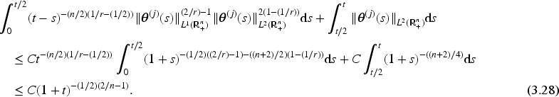
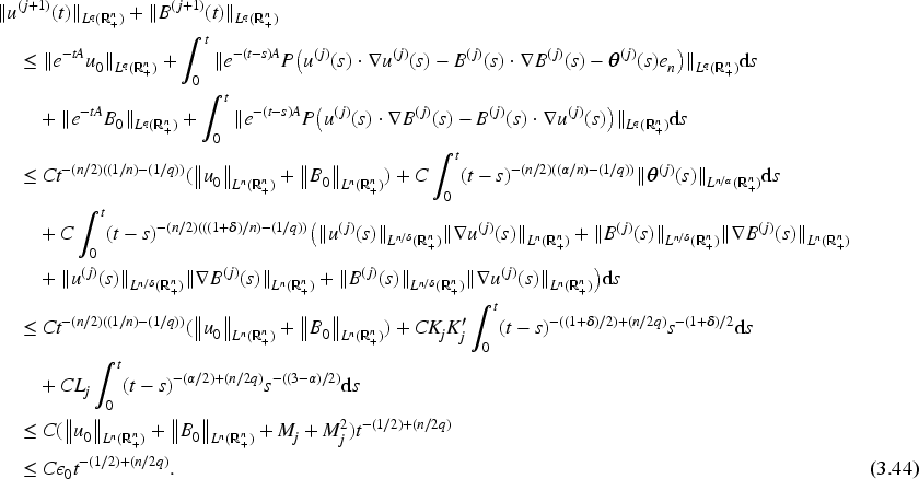
From (3.44), (3.46), and Lemma 2.4, we obtain for any

j = 0, 1, 2, \dots

and

t > 0

\begin{aligned} ‖ \nabla u^{(j + 1)} (t) ‖_{L^{\infty} (R_{+}^{n})} + ‖ \nabla B^{(j + 1)} (t) ‖_{L^{\infty} (R_{+}^{n})} \\ \leq ‖ \nabla e^{- (t / 2) A} u^{(j + 1)} (\frac{t}{2}) ‖_{L^{\infty} (R_{+}^{n})} + ‖ \nabla e^{- (t / 2) A} B^{(j + 1)} (\frac{t}{2}) ‖_{L^{\infty} (R_{+}^{n})} \\ + \int_{t / 2}^{t} ‖ \nabla e^{- (t - s) A} P (u^{(j)} (s) \cdot \nabla u^{(j)} (s) - B^{(j)} (s) \cdot \nabla B^{(j)} (s) - θ^{(j)} (s) e_{n}) ‖_{L^{\infty} (R_{+}^{n})} d s \\ + \int_{t / 2}^{t} ‖ \nabla e^{- (t - s) A} P (u^{(j)} (s) \cdot \nabla B^{(j)} (s) - B^{(j)} (s) \cdot \nabla u^{(j)} (s)) ‖_{L^{\infty} (R_{+}^{n})} d s \\ \leq C t^{- (1 / 2)} (‖ u^{(j + 1)} (\frac{t}{2}) ‖_{L^{\infty} (R_{+}^{n})} + ‖ B^{(j + 1)} (\frac{t}{2}) ‖_{L^{\infty} (R_{+}^{n})}) + C \int_{t / 2}^{t} (t - s)^{- (3 / 4)} ‖ θ^{(j)} (s) ‖_{L^{2 n} (R_{+}^{n})} d s \\ + C \int_{t / 2}^{t} (t - s)^{- (3 / 4)} (‖ u^{(j)} (s) ‖_{L^{2 n} (R_{+}^{n})} + ‖ B^{(j)} (s) ‖_{L^{2 n} (R_{+}^{n})}) (‖ \nabla u^{(j)} (s) ‖_{L^{\infty} (R_{+}^{n})} + ‖ \nabla B^{(j)} (s) ‖_{L^{\infty} (R_{+}^{n})}) d s \\ \leq C ϵ_{0} t^{- 1} + C ϵ_{0} Q_{j} (t) \int_{t / 2}^{t} (t - s)^{- (3 / 4)} s^{- (5 / 4)} d s + C ϵ_{0} \int_{t / 2}^{t} (t - s)^{- (3 / 4)} s^{- (5 / 4)} d s \\ \leq C ϵ_{0} t^{- 1} + C ϵ_{0} Q_{j} (t) t^{- 1}, \end{aligned}

(3.55)

where

Q_{j} (t) = sup_{0 < s \leq t} (s (‖ \nabla u^{(j)} (s) ‖_{L^{\infty} R_{+}^{n}} + ‖ \nabla B^{(j)} (s) ‖_{L^{\infty} R_{+}^{n}}))

. Therefore, by choosing

C ϵ_{0} \leq (1 / 2)

, we can easily obtain

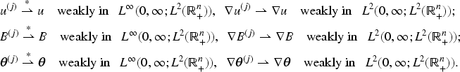
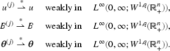
\begin{aligned} ‖ \nabla u^{(j + 1)} (t) ‖_{L^{\infty} (R_{+}^{n})} + ‖ \nabla B^{(j + 1)} (t) ‖_{L^{\infty} (R_{+}^{n})} \leq C ϵ_{0} t^{- 1} . \end{aligned}

(3.56)

From (3.44), (3.46), (3.48), (3.49), (3.54), (3.56), by using the weak convergence properties, we can find a subsequence $(u^{(j)}, B^{(j)}, θ^{(j)})$ of $(u, B, θ)$ as $j ⟶ \infty$

\begin{aligned} u^{(j)} \overset{*}{⇀} u & weakly in L^{\infty} (0, \infty; W^{1, q} (R_{+}^{n})), \\ B^{(j)} \overset{*}{⇀} B & weakly in L^{\infty} (0, \infty; W^{1, q} (R_{+}^{n})), \\ θ^{(j)} \overset{*}{⇀} θ & weakly in L^{\infty} (0, \infty; W^{1, q} (R_{+}^{n})) . \end{aligned}

Moreover, we can derive for

n \leq q \leq \infty

and

t > 0

by applying the limit under the weak convergence norm

\begin{aligned} {‖ u (t) ‖}_{L^{q} (R_{+}^{n})} + {‖ B (t) ‖}_{L^{q} (R_{+}^{n})} \leq \underset{j ⟶ \infty}{lim inf} (‖ u^{(j + 1)} (t) ‖_{L^{q} (R_{+}^{n})} + ‖ B^{(j + 1)} (t) ‖_{L^{q} (R_{+}^{n})}) \leq C ϵ_{0} t^{- (n / 2) ((1 / n) - (1 / q))}, \\ {‖ \nabla u (t) ‖}_{L^{q} (R_{+}^{n})} + {‖ \nabla B (t) ‖}_{L^{q} (R_{+}^{n})} \leq \underset{j ⟶ \infty}{lim inf} (‖ \nabla u^{(j + 1)} (t) ‖_{L^{q} (R_{+}^{n})} + ‖ \nabla B^{(j + 1)} (t) ‖_{L^{q} (R_{+}^{n})}) \leq C ϵ_{0} t^{- 1 + (n / 2 q)}, \\ {‖ θ (t) ‖}_{L^{q} (R_{+}^{n})} \leq \underset{j ⟶ \infty}{lim inf} ‖ θ^{(j + 1)} (t) ‖_{L^{q} (R_{+}^{n})} \leq C ϵ_{0} t^{- (3 / 2) + (n / 2 q)}, \\ {‖ \nabla θ (t) ‖}_{L^{q} (R_{+}^{n})} \leq \underset{j ⟶ \infty}{lim inf} ‖ \nabla θ^{(j + 1)} (t) ‖_{L^{q} (R_{+}^{n})} \leq C ϵ_{0} t^{- 2 + (n / 2 q)} . \end{aligned}

In conclusion, we can easily establish that $(u, B, θ)$ is a strong solution to problem (1.1) by combining parabolic regularity and the Serrin criteria. Additionally, $(u, B, θ)$ satisfies the estimates stated in Theorem 1.2.

3.3.

L^{q}

-Decay of Strong Solutions Without Smallness Conditions

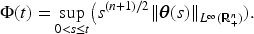
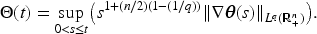
This section is devoted to investigating the $L^{q}$ -decay properties of strong solutions without smallness conditions. Based on Theorem 1.2, we relax the initial conditions and refine the required function spaces, thereby providing a basis for the subsequent derivation of Theorem 1.4. First, we introduce an auxiliary proposition to assist in completing the proof of the theorem.

Proposition 3.1
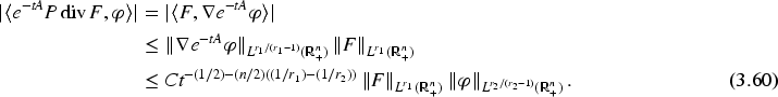
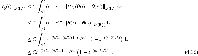
Let $u_{0}, B_{0} \in L_{σ}^{n} (R_{+}^{n}) \cap L^{(n / (n - 1))} (R_{+}^{n})$ and $θ_{0} \in L^{1} (R_{+}^{n}) \cap L^{2} (R_{+}^{n}) \cap L^{n / 3} (R_{+}^{n})$ , $n \geq 3$ and $(u, B, θ)$ is the strong solution to problem (1.1) obtained in Theorem 1.2. Assume (1.4) holds, then for $n / (n - 1) \leq r < 2$ , $r \leq q \leq \infty$ and $t > 0$ ,
$\begin{aligned} ‖ \nabla^{k} u (t) ‖_{L^{q} (R_{+}^{n})} + ‖ \nabla^{k} B (t) ‖_{L^{q} (R_{+}^{n})} \leq C t^{- (k / 2) - (n / 2) ((1 / r) - (1 / q))} for k = 0, 1. \end{aligned}$
(3.57)

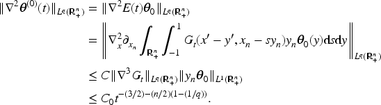
Proof. We first establish the $L^{r}$ -norm estimates of $u, B$ , which is crucial for proving the proposition. Then, we give an auxiliary estimate as follows:

Auxiliary estimates: Set
$\begin{aligned} L (q, r, t) = sup_{0 < s \leq t} (s^{(n / 2) ((1 / r) - (1 / q))} ({‖ u (s) ‖}_{L^{q} (R_{+}^{n})} + {‖ B (s) ‖}_{L^{q} (R_{+}^{n})})) . \end{aligned}$
(3.58)
Let $1 < r_{1} \leq r_{2} < \infty$ . Then
$\begin{aligned} ‖ e^{- t A} P div F ‖_{L^{r_{2}} (R_{+}^{n})} \leq C t^{- (1 / 2) - (n / 2) ((1 / r_{1}) - (1 / r_{2}))} {‖ F ‖}_{L^{r_{1}} (R_{+}^{n})} . \end{aligned}$
(3.59)
By Lemma 2.4, it follows that
$\begin{aligned} | ⟨ e^{- t A} P div F, φ ⟩ | & = | ⟨ F, \nabla e^{- t A} φ ⟩ | \\ \leq ‖ \nabla e^{- t A} φ ‖_{L^{r_{1} / (r_{1} - 1)} (R_{+}^{n})} {‖ F ‖}_{L^{r_{1}} (R_{+}^{n})} \\ \leq C t^{- (1 / 2) - (n / 2) ((1 / r_{1}) - (1 / r_{2}))} {‖ F ‖}_{L^{r_{1}} (R_{+}^{n})} {‖ φ ‖}_{L^{r_{2} / (r_{2} - 1)} (R_{+}^{n})} . \end{aligned}$
(3.60)
From Theorem 1.1, we know that ${‖ u (t) ‖}_{L^{2} (R_{+}^{n})} + {‖ B (t) ‖}_{L^{2} (R_{+}^{n})} \leq C_{ϵ} (1 + t)^{- ((n - 2) / 4) + ϵ}$ . By combining (3.59) and Theorem 1.2, we obtain
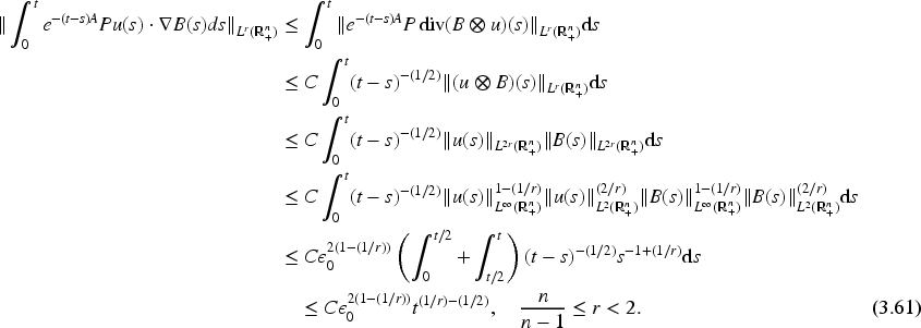
$\begin{aligned} ‖ \int_{0}^{t} e^{- (t - s) A} P u (s) \cdot \nabla B (s) d s ‖_{L^{r} (R_{+}^{n})} & \leq \int_{0}^{t} ‖ e^{- (t - s) A} P div (B \otimes u) (s) ‖_{L^{r} (R_{+}^{n})} d s \\ \leq C \int_{0}^{t} (t - s)^{- (1 / 2)} ‖ (u \otimes B) (s) ‖_{L^{r} (R_{+}^{n})} d s \\ \leq C \int_{0}^{t} (t - s)^{- (1 / 2)} ‖ u (s) ‖_{L^{2 r} (R_{+}^{n})} ‖ B (s) ‖_{L^{2 r} (R_{+}^{n})} d s \\ \leq C \int_{0}^{t} (t - s)^{- (1 / 2)} ‖ u (s) ‖_{L^{\infty} (R_{+}^{n})}^{1 - (1 / r)} ‖ u (s) ‖_{L^{2} (R_{+}^{n})}^{(2 / r)} ‖ B (s) ‖_{L^{\infty} (R_{+}^{n})}^{1 - (1 / r)} ‖ B (s) ‖_{L^{2} (R_{+}^{n})}^{(2 / r)} d s \\ \leq C ϵ_{0}^{2 (1 - (1 / r))} (\int_{0}^{t / 2} + \int_{t / 2}^{t}) (t - s)^{- (1 / 2)} s^{- 1 + (1 / r)} d s \\ \leq C ϵ_{0}^{2 (1 - (1 / r))} t^{(1 / r) - (1 / 2)}, \frac{n}{n - 1} \leq r < 2. \end{aligned}$
(3.61)

$L^{r}$ estimates of $u, B .$ Obviously, we have for $t > 0$
$\begin{aligned} u (t) = e^{- t A} u_{0} - \int_{0}^{t} e^{- (t - s) A} P (u (s) \cdot \nabla u (s) - B (s) \cdot \nabla B (s) - θ (s) e_{n}) d s, \\ B (t) = e^{- t A} B_{0} - \int_{0}^{t} e^{- (t - s) A} P (u (s) \cdot \nabla B (s) - B (s) \cdot \nabla u (s)) d s . \end{aligned}$
Using Theorem 1.1, Lemma 2.4, and (3.61), we get for $t > 0$
$\begin{aligned} {‖ u (t) ‖}_{L^{r} (R_{+}^{n})} + {‖ B (t) ‖}_{L^{r} (R_{+}^{n})} \\ \leq ‖ e^{- t A} u_{0} ‖_{L^{r} (R_{+}^{n})} + ‖ e^{- t A} B_{0} ‖_{L^{r} (R_{+}^{n})} + C \int_{0}^{t} (t - s)^{- (n / 2) ((1 / r) - (1 / 2))} ‖ θ (s) ‖_{L^{1} (R_{+}^{n})}^{(2 / r) - 1} ‖ θ (s) ‖_{L^{2} (R_{+}^{n})}^{2 (1 - (1 / r))} d s \\ + {‖ \int_{0}^{t} e^{- (t - s) A} P (u (s) \cdot \nabla u (s) - B (s) \cdot \nabla B (s)) d s ‖}_{L^{r} (R_{+}^{n})} \\ + {‖ \int_{0}^{t} e^{- (t - s) A} P (u (s) \cdot \nabla B (s) - B (s) \cdot \nabla u (s)) d s ‖}_{L^{r} (R_{+}^{n})} \\ \leq C ({‖ u_{0} ‖}_{L^{r} (R_{+}^{n})} + {‖ B_{0} ‖}_{L^{r} (R_{+}^{n})}) + C ϵ_{0}^{2 (1 - (1 / r))} t^{(1 / r) - (1 / 2)} + C \int_{0}^{t / 2} (1 + s)^{- (1 / 2) ((2 / r) - 1) - ((n + 2) / 2) (1 - (1 / r))} d s \\ \leq C ({‖ u_{0} ‖}_{L^{r} (R_{+}^{n})} + {‖ B_{0} ‖}_{L^{r} (R_{+}^{n})} + ϵ_{0}^{2 (1 - (1 / r))} t^{(1 / r) - (1 / 2)} + \log_{e} (1 + t)), \end{aligned}$
which implies that
$\begin{aligned} L (r, r, t) = sup_{0 < s \leq t} ({‖ u (s) ‖}_{L^{r} (R_{+}^{n})} + {‖ B (s) ‖}_{L^{r} (R_{+}^{n})}) \leq C (t) < \infty . \end{aligned}$
(3.62)
It is noted that $lim_{t \to \infty} C (t) = \infty$ , which implies the occurrence of a blow-up phenomenon. Although we have shown that the $L^{r}$ -norms of $u$ and $B$ are bounded in finite time, their uniform boundedness estimates have not yet been established. Next, we will accomplish this task. Let $n / (n - 1) \leq r < 2$ , it implies that $u_{0}, B_{0} \in L^{r} (R_{+}^{n})$ , we also obtain ${‖ θ (t) ‖}_{L^{1} (R_{+}^{n})} \leq C (1 + t)^{- (1 / 2)}, t > 0$ . Combining Lemma 2.4 and Theorem 1.1, we have for $r = n / (n - 1)$
$\begin{aligned} \int_{0}^{t} ‖ e^{- (t - s) A} P θ (s) e_{n} ‖_{L^{(n / (n - 1))} (R_{+}^{n})} d s \\ \leq C \int_{0}^{t} (t - s)^{- (n / 2) (1 - ((n - 1) / n))} ‖ θ (s) ‖_{L^{1} (R_{+}^{n})} d s + C \int_{t / 2}^{t} ‖ θ (s) ‖_{L^{1} (R_{+}^{n})}^{1 - (2 / n)} ‖ θ (s) ‖_{L^{2} (R_{+}^{n})}^{2 / n} d s \\ \leq C t^{- (1 / 2)} \int_{0}^{t} (1 + s)^{- (1 / 2)} + C \int_{t / 2}^{t} (1 + s)^{- (1 / 2) (1 - (2 / n)) - ((n + 2) / 2 n)} d s \\ \leq C \end{aligned}$
and $n / (n - 1) < r < 2$
$\begin{aligned} \int_{0}^{t} ‖ e^{- (t - s) A} P θ (s) e_{n} ‖_{L^{r} (R_{+}^{n})} d s & \leq C \int_{0}^{\infty} ‖ θ (s) ‖_{L^{1} (R_{+}^{n})}^{(2 / r) - 1} ‖ θ (s) ‖_{L^{2} (R_{+}^{n})}^{2 (1 - (1 / r))} d s \\ \leq C \int_{0}^{\infty} (1 + s)^{- (1 / 2) ((2 / r) - 1) - ((n + 2) / 2) (1 - (1 / r))} d s \\ \leq C . \end{aligned}$
It follows from the above estimate that for $t > 0$
$\begin{aligned} {‖ u (t) ‖}_{L^{r} (R_{+}^{n})} + {‖ B (t) ‖}_{L^{r} (R_{+}^{n})} \\ \leq ‖ e^{- t A} u_{0} ‖_{L^{r} (R_{+}^{n})} + ‖ e^{- t A} B_{0} ‖_{L^{r} (R_{+}^{n})} + C \int_{0}^{t} ‖ e^{- (t - s) A} P θ (s) e_{n} ‖_{L^{r}} d s \\ + C \int_{0}^{t} (t - s)^{- (1 / 2)} ({‖ u (s) ‖}_{L^{r} (R_{+}^{n})} + {‖ B (s) ‖}_{L^{r} (R_{+}^{n})}) ({‖ \nabla u (s) ‖}_{L^{n} (R_{+}^{n})} + {‖ \nabla B (s) ‖}_{L^{n} (R_{+}^{n})}) d s \\ \leq C (1 + {‖ u_{0} ‖}_{L^{r} (R_{+}^{n})} + {‖ B_{0} ‖}_{L^{r} (R_{+}^{n})}) + C ϵ_{0} L (r, r, t) \int_{0}^{t} (t - s)^{- (1 / 2)} s^{- (1 / 2)} d s \\ \leq C (1 + {‖ u_{0} ‖}_{L^{r} (R_{+}^{n})} + {‖ B_{0} ‖}_{L^{r} (R_{+}^{n})}) + C ϵ_{0} L (r, r, t) . \end{aligned}$
Thus, we have
$\begin{aligned} L (r, r, t) \leq C (1 + {‖ u_{0} ‖}_{L^{r} (R_{+}^{n})} + {‖ B_{0} ‖}_{L^{r} (R_{+}^{n})}) + C ϵ_{0} L (r, r, t) . \end{aligned}$
(3.63)
Let $C ϵ_{0} \leq (1 / 2)$ , from (3.62) and (3.63), we get for $n / (n - 1) \leq r < 2$ and $t > 0$
$\begin{aligned} {‖ u (t) ‖}_{L^{r} (R_{+}^{n})} + {‖ B (t) ‖}_{L^{r} (R_{+}^{n})} \leq L (r, r, t) \leq 2 C (1 + {‖ u_{0} ‖}_{L^{r} (R_{+}^{n})} + {‖ B_{0} ‖}_{L^{r} (R_{+}^{n})}) . \end{aligned}$
(3.64)
Then, we establish the $L^{q}$ -norm estimate of $θ$ . We first derive the estimation of ${‖ θ (t) ‖}_{L^{\infty} (R_{+}^{n})}$ . Let $m > n$ , by Theorem 1.2, we conclude that
$\begin{aligned} {‖ θ (t) ‖}_{L^{\infty} (R_{+}^{n})} & \leq ‖ E (\frac{t}{2}) θ (\frac{t}{2}) ‖_{L^{q} (R_{+}^{n})} + C \int_{t / 2}^{t} ‖ \nabla G_{t - s} ‖_{L^{m / (m - 1)} (R^{n})} ‖ u (s) θ (s) ‖_{L^{m} (R_{+}^{n})} d s \\ \leq C t^{- (n / 2)} ‖ θ (\frac{t}{2}) ‖_{L^{1} (R_{+}^{n})} + C \int_{t / 2}^{t} (t - s)^{- (1 / 2) - (n / 2 m)} ‖ u (s) ‖_{L^{m} (R_{+}^{n})} ‖ θ (s) ‖_{L^{\infty} (R_{+}^{n})} d s \\ \leq C t^{- ((n + 1) / 2)} + C ϵ_{0} Φ (t) \int_{t / 2}^{t} (t - s)^{- (1 / 2) - (n / 2 m)} s^{- ((n + 1) / 2) - (n / 2) ((1 / n) - (1 / m))} d s \\ \leq C t^{- ((n + 1) / 2)} + C ϵ_{0} Φ (t) t^{- ((n + 1) / 2)}, \end{aligned}$
from which
$\begin{aligned} Φ (t) \leq C + C ϵ_{0} Φ (t), \end{aligned}$
(3.65)
where
$Φ (t) = sup_{0 < s \leq t} (s^{(n + 1) / 2} ‖ θ (s) ‖_{L^{\infty} (R_{+}^{n})}) .$
Let $C ϵ_{0} \leq (1 / 2)$ , we have
$\begin{aligned} {‖ θ (t) ‖}_{L^{\infty} (R_{+}^{n})} \leq C t^{- ((n + 1) / 2)} . \end{aligned}$
(3.66)

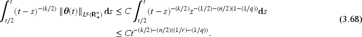
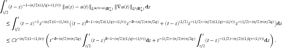
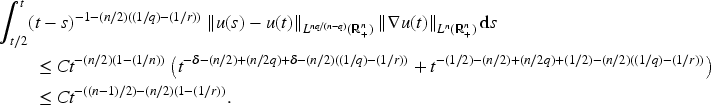
Decay of $θ \in L^{q}$ , $1 < q < \infty$ . From the interpolation inequality, we have
$\begin{aligned} {‖ θ (t) ‖}_{L^{q} (R_{+}^{n})} \leq {‖ θ (t) ‖}_{L^{1} (R_{+}^{n})}^{(1 / q)} {‖ θ (t) ‖}_{L^{\infty} (R_{+}^{n})}^{(q - 1) / q} \leq C t^{- (((n + 1) (q - 1)) / 2 q)} t^{- (1 / 2 q)} = C t^{- ((n + 1) / 2) + (n / 2 q)} = C t^{- (1 / 2) - (n / 2) (1 - (1 / q))} . \end{aligned}$
(3.67)

Decay of $u, B \in L^{q}$ , $n / (n - 1) \leq r < 2$ , $r \leq q \leq \infty$ . By (3.67), we have the auxiliary estimates for $k = 0, 1$ and any $t > 0$
$\begin{aligned} \begin{aligned} \int_{t / 2}^{t} (t - s)^{- (k / 2)} {‖ θ (t) ‖}_{L^{q} (R_{+}^{n})} d s & \leq C \int_{t / 2}^{t} (t - s)^{- (k / 2)} s^{- (1 / 2) - (n / 2) (1 - (1 / q))} d s \\ \leq C t^{- (k / 2) - (n / 2) ((1 / r) - (1 / q))} . \end{aligned} \end{aligned}$
(3.68)
From Lemma 2.4, Theorem 1.2, (3.64), and (3.68), we get for $0 < β \leq 1$ , $k = 0, 1$ and $t > 0$
$\begin{aligned} ‖ \nabla^{k} u (t) ‖_{L^{q} (R_{+}^{n})} + ‖ \nabla^{k} B (t) ‖_{L^{q} (R_{+}^{n})} \\ \leq ‖ \nabla^{k} e^{- (t / 2) A} u (\frac{t}{2}) ‖_{L^{q} (R_{+}^{n})} + ‖ \nabla^{k} e^{- (t / 2) A} B (\frac{t}{2}) ‖_{L^{q} (R_{+}^{n})} \\ + {‖ \int_{t / 2}^{t} \nabla^{k} e^{- (t - s) A} P (u (s) \cdot \nabla u (s) - B (s) \cdot \nabla B (s) - θ (s) e_{n}) d s ‖}_{L^{q} (R_{+}^{n})} \\ + {‖ \int_{t / 2}^{t} \nabla^{k} e^{- (t - s) A} P (u (s) \cdot \nabla B (s) - B (s) \cdot \nabla u (s)) d s ‖}_{L^{q} (R_{+}^{n})} \\ \leq C t^{- (k / 2) - (n / 2) ((1 / r) - (1 / q))} ({‖ u (\frac{t}{2}) ‖}_{L^{r} (R_{+}^{n})} + {‖ B (\frac{t}{2}) ‖}_{L^{r} (R_{+}^{n})}) + C \int_{t / 2}^{t} (t - s)^{- (k / 2)} {‖ θ (s) ‖}_{L^{q} (R_{+}^{n})} d s \\ + C \int_{t / 2}^{t} (t - s)^{- (k / 2) - (β / 2)} ({‖ u (s) ‖}_{L^{q} (R_{+}^{n})} + {‖ B (s) ‖}_{L^{q} (R_{+}^{n})}) ({‖ \nabla u (s) ‖}_{L^{n / β} (R_{+}^{n})} + {‖ \nabla B (s) ‖}_{L^{n / β} (R_{+}^{n})}) d s . \end{aligned}$
(3.69)
Let $k = 0 and β = 1$ , we obtain by combining the decay estimate for $‖ \nabla u ‖_{L^{n} (R_{+}^{n})}$ in Theorem 1.2
$\begin{aligned} ‖ u (t) ‖_{L^{q} (R_{+}^{n})} + ‖ B (t) ‖_{L^{q} (R_{+}^{n})} & \leq C t^{- (n / 2) ((1 / r) - (1 / q))} + C ϵ_{0} Ψ (t) \int_{t / 2}^{t} (t - s)^{- (1 / 2)} s^{- (1 / 2) - (n / 2) ((1 / r) - (1 / q))} d s \\ \leq C t^{- (n / 2) ((1 / r) - (1 / q))} + C ϵ_{0} Ψ (t) t^{- (n / 2) ((1 / r) - (1 / q))}, \end{aligned}$
(3.70)
from which
$Ψ (t) \leq C + C ϵ_{0} Ψ (t), where Ψ (t) = sup_{0 < s \leq t} (s^{(n / 2) ((1 / r) - (1 / q))} (‖ u (s) ‖_{L^{q} (R_{+}^{n})} + ‖ B (s) ‖_{L^{q} (R_{+}^{n})}) .$
By choosing $C ϵ_{0} \leq (1 / 2)$ , we obtain
$\begin{aligned} ‖ u (t) ‖_{L^{q} (R_{+}^{n})} + ‖ B (t) ‖_{L^{q} (R_{+}^{n})} \leq C t^{- (n / 2) ((1 / r) - (1 / q))} . \end{aligned}$
(3.71)
Let $k = 1 and β = (1 / 2)$ , we arrive at
$\begin{aligned} ‖ \nabla u (t) ‖_{L^{q} (R_{+}^{n})} + ‖ \nabla B (t) ‖_{L^{q} (R_{+}^{n})} & \leq C t^{- (1 / 2) - (n / 2) ((1 / r) - (1 / q))} + C \int_{t / 2}^{t} (t - s)^{- (1 / 2) - (1 / 4)} s^{- (1 / 2) - (1 / 4) - (n / 2) ((1 / r) - (1 / q))} d s \\ \leq C t^{- (1 / 2) - (n / 2) ((1 / r) - (1 / q))} . \end{aligned}$
(3.72)
The proof of Proposition 3.1 is complete. □

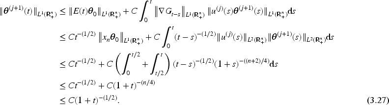
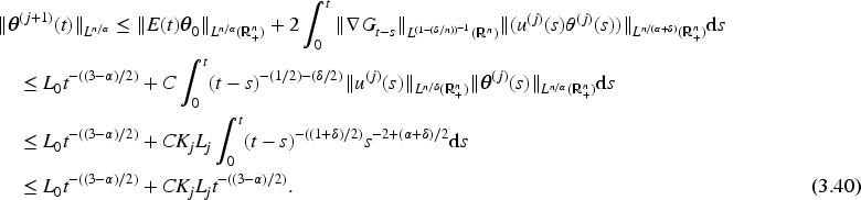
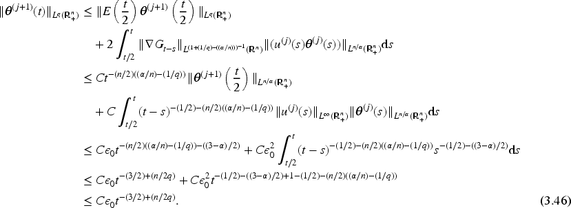
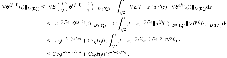
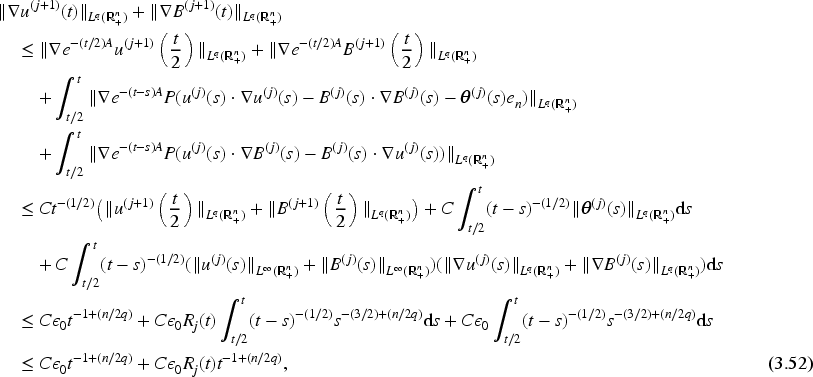
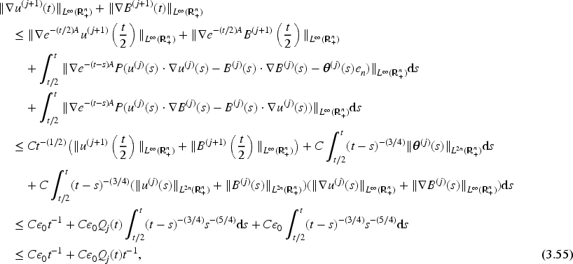
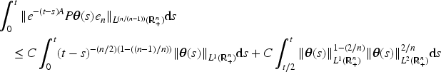
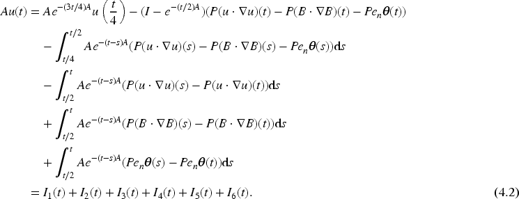
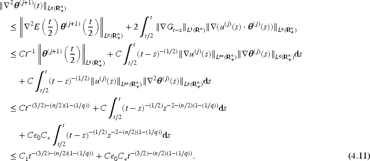
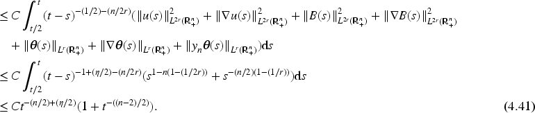
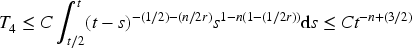
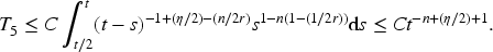
Proof of Theorem 1.3. The estimation of ${‖ θ ‖}_{L^{q} (R_{+}^{n})}$ has been accomplished in the preceding text; our next core work is to complete the estimate of $‖ \nabla θ (t) ‖_{L^{q} (R_{+}^{n})}$ . Theorem 1.2 and (3.3) yield for $1 \leq q \leq \infty$ and any $t > 0$ .
$\begin{aligned} ‖ \nabla θ (t) ‖_{L^{q} (R_{+}^{n})} & \leq {‖ \nabla E (\frac{t}{2}) θ (\frac{t}{2}) ‖}_{L^{q} (R_{+}^{n})} + \int_{t / 2}^{t} ‖ \nabla E (t - s) (u (s) \cdot \nabla θ (s)) ‖_{L^{q} (R_{+}^{n})} d s \\ \leq C t^{- (1 / 2)} ‖ θ (t) ‖_{L^{q} (R_{+}^{n})} + C \int_{t / 2}^{t} (t - s)^{- (3 / 4)} ‖ u (s) ‖_{L^{2 n} (R_{+}^{n})} ‖ \nabla θ (s) ‖_{L^{q} (R_{+}^{n})} d s \\ \leq C t^{- 1 - (n / 2) (1 - (1 / q))} + C ϵ_{0} Θ (t) \int_{t / 2}^{t} (t - s)^{- (3 / 4)} s^{- (5 / 4) - (n / 2) (1 - (1 / q))} d s \\ \leq C t^{- 1 - (n / 2) (1 - (1 / q))} + C ϵ_{0} Θ (t) t^{- 1 - (n / 2) (1 - (1 / q))}, \end{aligned}$
from which
$\begin{aligned} Θ (t) \leq C + C ϵ_{0} Θ (t), \end{aligned}$
(3.73)
where
$Θ (t) = sup_{0 < s \leq t} (s^{1 + (n / 2) (1 - (1 / q))} ‖ \nabla θ (s) ‖_{L^{q} (R_{+}^{n})}) .$
Take $ϵ_{0} > 0$ such that $C ϵ_{0} \leq (1 / 2)$ . Then, for $1 \leq q \leq \infty$ and $t > 0$
$\begin{aligned} ‖ \nabla θ (s) ‖_{L^{q} (R_{+}^{n})} \leq C t^{- 1 - (n / 2) (1 - (1 / q))} . \end{aligned}$
(3.74)
Let $r = n / (n - 1)$ in (3.71) and (3.72), we obtain
$\begin{aligned} ‖ \nabla^{k} u (s) ‖_{L^{q} (R_{+}^{n})} + ‖ \nabla^{k} B (s) ‖_{L^{q} (R_{+}^{n})} \leq C t^{- ((k - 1) / 2) - (n / 2) (1 - (1 / q))}, k = 0, 1. \end{aligned}$
(3.75)
We complete the proof of Theorem 1.3. □
4. Decay Estimates of High Order Derivatives

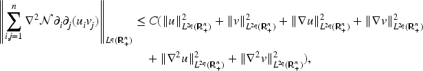
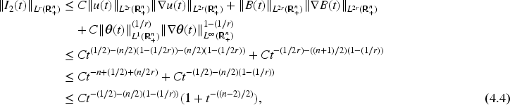
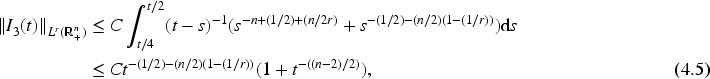
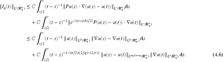
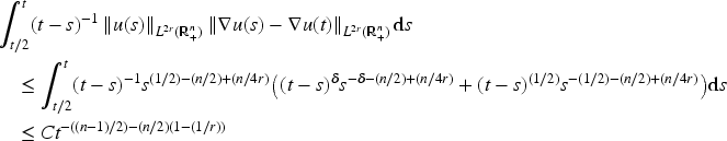
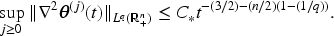
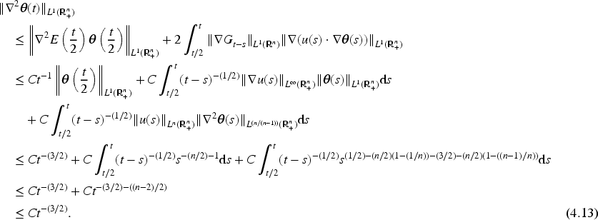
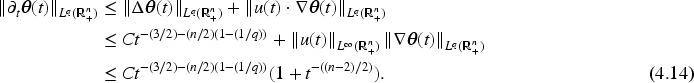
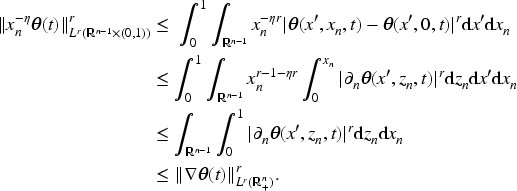
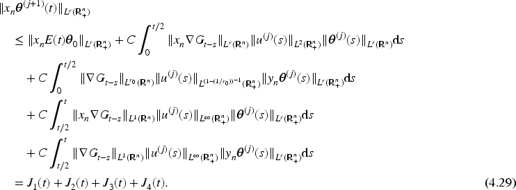
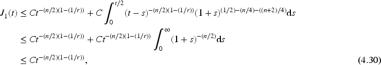
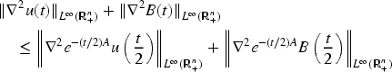
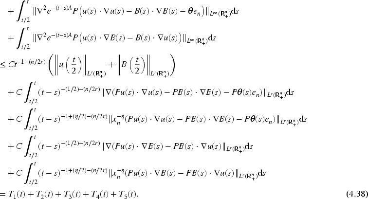
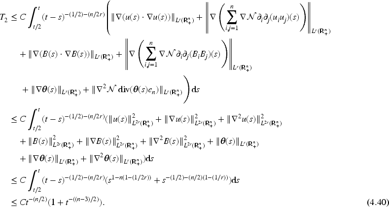
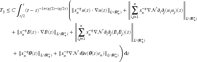
In this section, our main aim is to estimate the decay of the second spatial order derivatives and the decay of the third derivative of $θ$ for $t > 0$ . Specifically, for the first part of Theorem 1.4, we prove it by means of an auxiliary lemma.

Lemma 4.1

Let $u_{0}, B_{0} \in L_{σ}^{n} (R_{+}^{n}) \cap L^{(n / (n - 1))} (R_{+}^{n})$ and $θ_{0} \in L^{1} (R_{+}^{n}) \cap L^{2} (R_{+}^{n}) \cap L^{n / 3} (R_{+}^{n})$ , $n \geq 3$ , $(u, B, θ)$ be the strong solution to problem (1.1) obtained in Theorem 1.2. Then, for $n / (n - 1) \leq r < \infty$

‖ \nabla^{2} u (t) ‖_{L^{r} (R_{+}^{n})} + ‖ \nabla^{2} B (t) ‖_{L^{r} (R_{+}^{n})} + {‖ \partial_{t} u (t) ‖}_{L^{r} (R_{+}^{n})} + {‖ \partial_{t} B (t) ‖}_{L^{r} (R_{+}^{n})} + {‖ \nabla p (t) ‖}_{L^{r} (R_{+}^{n})} \leq C t^{- (1 / 2) - (n / 2) (1 - (1 / r))},

and

‖ \nabla^{2} θ (t) ‖_{L^{r} (R_{+}^{n})} \leq C t^{- (3 / 2) - (n / 2) (1 - (1 / r))} for 1 \leq r \leq \infty .

Proof. Using the method proposed in Kozono and Ogawa (1992), we can establish for $0 < α < 1$ and $0 < δ < 1 - α$

\begin{aligned} ‖ A^{α} u (t + h) - A^{α} u (t) ‖_{L^{r} (R_{+}^{n})} + ‖ A^{α} B (t + h) - A^{α} B (t) ‖_{L^{r} (R_{+}^{n})} \\ \leq C (h^{δ} t^{- α - δ - (n / 2) + (1 / 2) + (n / 2 r)} + h^{1 - α} t^{- (1 / 2) - (n / 2) + (n / 2 r)}), \end{aligned}

(4.1)

where

1 < r < \infty

and

t > 0, h > 0

. This inequality is crucial for the subsequent estimation of

I_{4}

. Here, we decompose

A (u)

using the following method and arrive at

\begin{aligned} A u (t) & = A e^{- (3 t / 4) A} u (\frac{t}{4}) - (I - e^{- (t / 2) A}) (P (u \cdot \nabla u) (t) - P (B \cdot \nabla B) (t) - P e_{n} θ (t)) \\ - \int_{t / 4}^{t / 2} A e^{- (t - s) A} (P (u \cdot \nabla u) (s) - P (B \cdot \nabla B) (s) - P e_{n} θ (s)) d s \\ - \int_{t / 2}^{t} A e^{- (t - s) A} (P (u \cdot \nabla u) (s) - P (u \cdot \nabla u) (t)) d s \\ + \int_{t / 2}^{t} A e^{- (t - s) A} (P (B \cdot \nabla B) (s) - P (B \cdot \nabla B) (t)) d s \\ + \int_{t / 2}^{t} A e^{- (t - s) A} (P e_{n} θ (s) - P e_{n} θ (t)) d s \\ = I_{1} (t) + I_{2} (t) + I_{3} (t) + I_{4} (t) + I_{5} (t) + I_{6} (t) . \end{aligned}

(4.2)

We next turn to estimate

I_{i}, i = 1, 2, 3, 4, 5, 6

. Let

n / (n - 1) \leq r < \infty

, by Lemma 2.4 and Theorem 1.2, we have for any

t > 0

\begin{aligned} ‖ I_{1} (t) ‖_{L^{r} (R_{+}^{n})} & \leq C t^{- 1} {‖ u (\frac{t}{4}) ‖}_{L^{r} (R_{+}^{n})} \leq C t^{- (1 / 2) - (n / 2) (1 - (1 / r))}, \end{aligned}

(4.3)

\begin{aligned} ‖ I_{2} (t) ‖_{L^{r} (R_{+}^{n})} & \leq C ‖ u (t) ‖_{L^{2 r} (R_{+}^{n})} ‖ \nabla u (t) ‖_{L^{2 r} (R_{+}^{n})} + ‖ B (t) ‖_{L^{2 r} (R_{+}^{n})} ‖ \nabla B (t) ‖_{L^{2 r} (R_{+}^{n})} \\ + C ‖ θ (t) ‖_{L^{1} (R_{+}^{n})}^{(1 / r)} ‖ \nabla θ (t) ‖_{L^{\infty} (R_{+}^{n})}^{1 - (1 / r)} \\ \leq C t^{(1 / 2) - (n / 2) (1 - (1 / 2 r)) - (n / 2) (1 - (1 / 2 r))} + C t^{- (1 / 2 r) - ((n + 1) / 2) (1 - (1 / r))} \\ \leq C t^{- n + (1 / 2) + (n / 2 r)} + C t^{- (1 / 2) - (n / 2) (1 - (1 / r))} \\ \leq C t^{- (1 / 2) - (n / 2) (1 - (1 / r))} (1 + t^{- ((n - 2) / 2)}), \end{aligned}

(4.4)

\begin{aligned} ‖ I_{3} (t) ‖_{L^{r} (R_{+}^{n})} & \leq C \int_{t / 4}^{t / 2} (t - s)^{- 1} (s^{- n + (1 / 2) + (n / 2 r)} + s^{- (1 / 2) - (n / 2) (1 - (1 / r))}) d s \\ \leq C t^{- (1 / 2) - (n / 2) (1 - (1 / r))} (1 + t^{- ((n - 2) / 2)}), \end{aligned}

(4.5)

\begin{aligned} ‖ I_{4} (t) ‖_{L^{r} (R_{+}^{n})} & \leq C \int_{t / 2}^{t} (t - s)^{- 1} ‖ P u (s) \cdot \nabla (u (s) - u (t)) ‖_{L^{r} (R_{+}^{n})} d s \\ + C \int_{t / 2}^{t} (t - s)^{- 1} ‖ e^{- ((t - s) A) / 2)} P (u (s) - u (t)) \cdot \nabla u (t) ‖_{L^{r} (R_{+}^{n})} \\ \leq C \int_{t / 2}^{t} (t - s)^{- 1} {‖ u (s) ‖}_{L^{2 r} (R_{+}^{n})} {‖ \nabla u (s) - \nabla u (t) ‖}_{L^{2 r} (R_{+}^{n})} d s \\ + C \int_{t / 2}^{t} (t - s)^{- 1 - (n / 2) ((1 / q) - (1 / r))} {‖ u (s) - u (t) ‖}_{L^{n q / (n - q)} (R_{+}^{n})} {‖ \nabla u (t) ‖}_{L^{n} (R_{+}^{n})} d s . \end{aligned}

(4.6)

Note that for

1 < q < n

\begin{aligned} {‖ φ ‖}_{L^{n q / (n - q)} (R_{+}^{n})} \leq C ‖ A^{(1 / 2)} φ ‖_{L^{q} (R_{+}^{n})}, \forall φ \in D (A^{(1 / 2)}) . \end{aligned}

(4.7)

We also note that

\begin{aligned} ‖ \nabla u (t) ‖_{L^{q} (R_{+}^{n})} \approx ‖ A^{(1 / 2)} u (t) ‖_{L^{q} (R_{+}^{n})}, 1 < q < \infty . \end{aligned}

(4.8)

Thus, by (4.1), (4.7), and (4.8), we have

\begin{aligned} \int_{t / 2}^{t} (t - s)^{- 1} {‖ u (s) ‖}_{L^{2 r} (R_{+}^{n})} {‖ \nabla u (s) - \nabla u (t) ‖}_{L^{2 r} (R_{+}^{n})} d s \\ \leq \int_{t / 2}^{t} (t - s)^{- 1} s^{(1 / 2) - (n / 2) + (n / 4 r)} ((t - s)^{δ} s^{- δ - (n / 2) + (n / 4 r)} + (t - s)^{(1 / 2)} s^{- (1 / 2) - (n / 2) + (n / 4 r)}) d s \\ \leq C t^{- ((n - 1) / 2) - (n / 2) (1 - (1 / r))} \end{aligned}

and

\begin{aligned} \int_{t / 2}^{t} (t - s)^{- 1 - (n / 2) ((1 / q) - (1 / r))} {‖ u (s) - u (t) ‖}_{L^{n q / (n - q)} (R_{+}^{n})} {‖ \nabla u (t) ‖}_{L^{n} (R_{+}^{n})} d s \\ \leq \int_{t / 2}^{t} (t - s)^{- 1} s^{- (n / 2) (1 - (1 / n))} ((t - s)^{δ - 1 - (n / 2) ((1 / q) - (1 / r))} s^{- δ - (n / 2) + (n / 2 q)} + (t - s)^{(1 / 2)} s^{- (1 / 2) - (n / 2) ((1 / q) - (1 / r))} s^{- (1 / 2) - (n / 2) + (n / 2 q)}) d s \\ \leq C t^{- (n / 2) (1 - (1 / n))} (t^{- δ - (n / 2) + (n / 2 q)} \int_{t / 2}^{t} (t - s)^{δ - 1 - (n / 2) ((1 / q) - (1 / r))} d s + t^{- (1 / 2) - (n / 2) + (n / 2 q)} \int_{t / 2}^{t} (t - s)^{- (1 / 2) - (n / 2) ((1 / q) - (1 / r))} d s) . \end{aligned}

Here, we require that

δ - (n / 2) ((1 / q) - (1 / r)) > 0

and

(1 / 2) - (n / 2) ((1 / q) - (1 / r)) > 0

. Thus, we derive

\begin{aligned} \int_{t / 2}^{t} (t - s)^{- 1 - (n / 2) ((1 / q) - (1 / r))} {‖ u (s) - u (t) ‖}_{L^{n q / (n - q)} (R_{+}^{n})} {‖ \nabla u (t) ‖}_{L^{n} (R_{+}^{n})} d s \\ \leq C t^{- (n / 2) (1 - (1 / n))} (t^{- δ - (n / 2) + (n / 2 q) + δ - (n / 2) ((1 / q) - (1 / r))} + t^{- (1 / 2) - (n / 2) + (n / 2 q) + (1 / 2) - (n / 2) ((1 / q) - (1 / r))}) \\ \leq C t^{- ((n - 1) / 2) - (n / 2) (1 - (1 / r))} . \end{aligned}

Similarly, we obtain

\begin{aligned} ‖ I_{4} (t) ‖_{L^{r} (R_{+}^{n})} \leq C t^{- ((n - 1) / 2) - (n / 2) (1 - (1 / r))}, \end{aligned}

(4.9)

and

\begin{aligned} ‖ I_{5} (t) ‖_{L^{r} (R_{+}^{n})} \leq C t^{- ((n - 1) / 2) - (n / 2) (1 - (1 / r))} . \end{aligned}

(4.10)

Next, we estimate $‖ \nabla^{2} θ (t) ‖_{L^{q} (R_{+}^{n})}$ by induction, a result that is crucial for the subsequent estimation of $I_{6}$ . Let $1 \leq q \leq \infty$ , using (3.36), we obtain for any $t > 0$

\begin{aligned} ‖ \nabla^{2} θ^{(0)} (t) ‖_{L^{q} (R_{+}^{n})} & = ‖ \nabla^{2} E (t) θ_{0} ‖_{L^{q} (R_{+}^{n})} \\ = {‖ \nabla_{x}^{2} \partial_{x_{n}} \int_{R_{+}^{n}} \int_{- 1}^{1} G_{t} (x^{'} - y^{'}, x_{n} - s y_{n}) y_{n} θ_{0} (y) d s d y ‖}_{L^{q} (R_{+}^{n})} \\ \leq C ‖ \nabla^{3} G_{t} ‖_{L^{q} (R_{+}^{n})} ‖ y_{n} θ_{0} ‖_{L^{1} (R_{+}^{n})} \\ \leq C_{0} t^{- (3 / 2) - (n / 2) (1 - (1 / q))} . \end{aligned}

We assume that there exists

j \geq 0

for which

‖ \nabla^{2} θ^{(j)} (t) ‖_{L^{q} (R_{+}^{n})} \leq C_{*} t^{- (3 / 2) - (n / 2) (1 - (1 / q))} .

Let

1 \leq q \leq \infty

, using Theorems 1.2 and 1.3, we get for any

t > 0

\begin{aligned} ‖ \nabla^{2} θ^{(j + 1)} (t) ‖_{L^{q} (R_{+}^{n})} \\ \leq {‖ \nabla^{2} E (\frac{t}{2}) θ^{(j + 1)} (\frac{t}{2}) ‖}_{L^{q} (R_{+}^{n})} + 2 \int_{t / 2}^{t} ‖ \nabla G_{t - s} ‖_{L^{1} (R^{n})} ‖ \nabla (u^{(j)} (s) \cdot θ^{(j)} (s)) ‖_{L^{q} (R_{+}^{n})} \\ \leq C t^{- 1} {‖ θ^{(j + 1)} (\frac{t}{2}) ‖}_{L^{q} (R_{+}^{n})} + C \int_{t / 2}^{t} (t - s)^{- (1 / 2)} ‖ \nabla u^{(j)} (s) ‖_{L^{\infty} (R_{+}^{n})} ‖ \nabla θ^{(j)} (s) ‖_{L^{q} (R_{+}^{n})} d s \\ + C \int_{t / 2}^{t} (t - s)^{- (1 / 2)} ‖ u^{(j)} (s) ‖_{L^{\infty} (R_{+}^{n})} ‖ \nabla^{2} θ^{(j)} (s) ‖_{L^{q} (R_{+}^{n})} d s \\ \leq C t^{- (3 / 2) - (n / 2) (1 - (1 / q))} + C \int_{t / 2}^{t} (t - s)^{- (1 / 2)} s^{- 2 - (n / 2) (1 - (1 / q))} d s \\ + C ϵ_{0} C_{*} \int_{t / 2}^{t} (t - s)^{- (1 / 2)} s^{- 2 - (n / 2) (1 - (1 / q))} d s \\ \leq C_{1} t^{- (3 / 2) - (n / 2) (1 - (1 / q))} + C ϵ_{0} C_{*} t^{- (3 / 2) - (n / 2) (1 - (1 / q))} . \end{aligned}

(4.11)

Choose

ϵ_{0} > 0

suitably small such that

C ϵ_{0} \leq (1 / 2)

in (4.11), let

C_{*} = C_{0} + 2 C_{1}

. Then, for

1 \leq q \leq \infty

and

t > 0

‖ \nabla^{2} θ^{(j + 1)} (t) ‖_{L^{q} (R_{+}^{n})} \leq C_{*} t^{- (3 / 2) - (n / 2) (1 - (1 / q))} .

By induction, we have proven that

sup_{j \geq 0} ‖ \nabla^{2} θ^{(j)} (t) ‖_{L^{q} (R_{+}^{n})} \leq C_{*} t^{- (3 / 2) - (n / 2) (1 - (1 / q))} .

We still apply the weak convergence theorem and get for each

t > 0

, as

j ⟶ \infty

\nabla^{2} θ^{(j)} \overset{*}{⇀} \nabla^{2} θ weakly in L^{q} (R_{+}^{n}), 1 \leq q \leq \infty .

Moreover, it holds that

\begin{aligned} ‖ \nabla^{2} θ (t) ‖_{L^{q} (R_{+}^{n})} \leq \underset{j ⟶ \infty}{lim inf} ‖ \nabla^{2} θ^{(j)} (t) ‖_{L^{q} (R_{+}^{n})} \leq C_{*} t^{- (3 / 2) - (n / 2) (1 - (1 / q))}, 1 < q \leq \infty . \end{aligned}

(4.12)

Now, we estimate the case

q = 1

as follows. Using

θ (t) = E (\frac{t}{2}) θ (\frac{t}{2}) - \int_{t / 2}^{t} E (t - s) P u (s) \cdot \nabla θ (s) d s .

Combining (4.12) and Theorem 1.3, we have

\begin{aligned} ‖ \nabla^{2} θ (t) ‖_{L^{1} (R_{+}^{n})} \\ \leq {‖ \nabla^{2} E (\frac{t}{2}) θ (\frac{t}{2}) ‖}_{L^{1} (R_{+}^{n})} + 2 \int_{t / 2}^{t} ‖ \nabla G_{t - s} ‖_{L^{1} (R^{n})} ‖ \nabla (u (s) \cdot \nabla θ (s)) ‖_{L^{1} (R_{+}^{n})} \\ \leq C t^{- 1} {‖ θ (\frac{t}{2}) ‖}_{L^{1} (R_{+}^{n})} + C \int_{t / 2}^{t} (t - s)^{- (1 / 2)} ‖ \nabla u (s) ‖_{L^{\infty} (R_{+}^{n})} ‖ θ (s) ‖_{L^{1} (R_{+}^{n})} d s \\ + C \int_{t / 2}^{t} (t - s)^{- (1 / 2)} ‖ u (s) ‖_{L^{n} (R_{+}^{n})} ‖ \nabla^{2} θ (s) ‖_{L^{(n / (n - 1))} (R_{+}^{n})} d s \\ \leq C t^{- (3 / 2)} + C \int_{t / 2}^{t} (t - s)^{- (1 / 2)} s^{- (n / 2) - 1} d s + C \int_{t / 2}^{t} (t - s)^{- (1 / 2)} s^{(1 / 2) - (n / 2) (1 - (1 / n)) - (3 / 2) - (n / 2) (1 - ((n - 1) / n))} d s \\ \leq C t^{- (3 / 2)} + C t^{- (3 / 2) - ((n - 2) / 2)} \\ \leq C t^{- (3 / 2)} . \end{aligned}

(4.13)

In order to estimate $I_{6}$ , securing the bound of $‖ \partial_{t} θ (t) ‖_{L^{q} (R_{+}^{n})}$ is essential. From the equation on $θ$ in (1.1), we get

\begin{aligned} ‖ \partial_{t} θ (t) ‖_{L^{q} (R_{+}^{n})} & \leq ‖ Δ θ (t) ‖_{L^{q} (R_{+}^{n})} + ‖ u (t) \cdot \nabla θ (t) ‖_{L^{q} (R_{+}^{n})} \\ \leq C t^{- (3 / 2) - (n / 2) (1 - (1 / q))} + {‖ u (t) ‖}_{L^{\infty} (R_{+}^{n})} {‖ \nabla θ (t) ‖}_{L^{q} (R_{+}^{n})} \\ \leq C t^{- (3 / 2) - (n / 2) (1 - (1 / q))} (1 + t^{- ((n - 2) / 2)}) . \end{aligned}

(4.14)

Thus, we obtain for

1 \leq q \leq \infty

and

0 < s \leq t

\begin{aligned} ‖ θ (t) - θ (s) ‖_{L^{q} (R_{+}^{n})} & \leq \int_{s}^{t} ‖ \partial_{τ} θ (τ) ‖_{L^{q} (R_{+}^{n})} d τ \leq \int_{s}^{t} τ^{- (3 / 2) - (n / 2) (1 - (1 / q))} (1 + τ^{- ((n - 2) / 2)}) d τ \\ \leq C (t - s) s^{- (3 / 2) - (n / 2) (1 - (1 / q))} (1 + s^{- ((n - 2) / 2)}) . \end{aligned}

(4.15)

From (4.15), it yields for any

n / (n - 1) \leq r < \infty

and

t > 0

\begin{aligned} ‖ I_{6} (t) ‖_{L^{r} (R_{+}^{n})} & \leq C \int_{t / 2}^{t} (t - s)^{- 1} ‖ P e_{n} (θ (t) - θ (s)) ‖_{L^{r} (R_{+}^{n})} d s \\ \leq C \int_{t / 2}^{t} (t - s)^{- 1} ‖ θ (t) - θ (s) ‖_{L^{r} (R_{+}^{n})} d s \\ \leq C \int_{t / 2}^{t} s^{- (3 / 2) - (n / 2) (1 - (1 / r))} (1 + s^{- ((n - 2) / 2)}) d s \\ \leq C t^{- (1 / 2) - (n / 2) (1 - (1 / r))} (1 + t^{- ((n - 2) / 2)}) . \end{aligned}

(4.16)

Combining the estimates for

‖ I_{i} (t) ‖_{L^{r} (R_{+}^{n})}, i = 1, 2, 3, 4, 5, 6

, we get for

t > 0

\begin{aligned} ‖ A u (t) ‖_{L^{r} (R_{+}^{n})} \leq C t^{- (1 / 2) - (n / 2) (1 - (1 / r))} for \frac{n}{n - 1} \leq r < \infty . \end{aligned}

(4.17)

By the known estimate in Borchers and Miyakawa (1988):

‖ \nabla^{2} u (t) ‖_{L^{q} (R_{+}^{n})} \leq C ‖ A u (t) ‖_{L^{q} (R_{+}^{n})}

q \in (1, \infty)

, we obtain

\begin{aligned} ‖ \nabla^{2} u (t) ‖_{L^{r} (R_{+}^{n})} \leq C t^{- (1 / 2) - (n / 2) (1 - (1 / r))} for \frac{n}{n - 1} \leq r < \infty . \end{aligned}

(4.18)

Since

\partial_{t} u (t) = - A u - P ((u \cdot \nabla u) (t) - (B \cdot \nabla B) (t) - e_{n} θ (t))

, we have for any

t > 0

\begin{aligned} ‖ \partial_{t} u (t) ‖_{L^{r} (R_{+}^{n})} & \leq ‖ A u (t) ‖_{L^{r} (R_{+}^{n})} + ‖ u (t) ‖_{L^{2 r} (R_{+}^{n})} ‖ \nabla u (t) ‖_{L^{2 r} (R_{+}^{n})} \\ + ‖ B (t) ‖_{L^{2 r} (R_{+}^{n})} ‖ \nabla B (t) ‖_{L^{2 r} (R_{+}^{n})} + ‖ θ (t) ‖_{L^{r} (R_{+}^{n})} \\ \leq C t^{- (1 / 2) - (n / 2) (1 - (1 / r))} for \frac{n}{n - 1} \leq r < \infty . \end{aligned}

(4.19)

Then, it follows from equation (1.1) that

\begin{aligned} ‖ \nabla p (t) ‖_{L^{r} (R_{+}^{n})} & \leq ‖ \partial_{t} u (t) ‖_{L^{r} (R_{+}^{n})} + ‖ \nabla^{2} u (t) ‖_{L^{r} (R_{+}^{n})} + ‖ u (t) ‖_{L^{2 r} (R_{+}^{n})} ‖ \nabla u (t) ‖_{L^{2 r} (R_{+}^{n})} \\ + ‖ B (t) ‖_{L^{2 r} (R_{+}^{n})} ‖ \nabla B (t) ‖_{L^{2 r} (R_{+}^{n})} + ‖ θ (t) ‖_{L^{r} (R_{+}^{n})} \\ \leq C t^{- (1 / 2) - (n / 2) (1 - (1 / r))} for \frac{n}{n - 1} \leq r < \infty . \end{aligned}

(4.20)

We can also have

\begin{aligned} ‖ \nabla^{2} B (t) ‖_{L^{r} (R_{+}^{n})} + {‖ \partial_{t} B (t) ‖}_{L^{r} (R_{+}^{n})} \leq C t^{- (1 / 2) - (n / 2) (1 - (1 / r))} . \end{aligned}

(4.21)

Combining the above-derived estimates, we finish the proof of Lemma 4.1. □

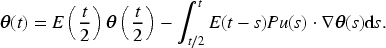
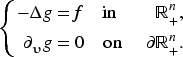
Now, we prove the rest of Theorem 1.4. Let $g = N f$ be the solution to the Neumann problem

{\begin{aligned} - Δ g & = f in & R_{+}^{n}, \\ \partial_{υ} g & = 0 on & \partial R_{+}^{n} . \end{aligned}

where

υ

is the unit outward normal vector of

\partial R_{+}^{n}

\begin{aligned} N = \int_{0}^{\infty} F (τ) d τ, \end{aligned}

(4.22)

and we define the operator

F

F (t) f (x) = \int_{R_{+}^{n}} [G_{t} (x^{'} - y^{'}, x_{n} - y_{n}) + G_{t} (x^{'} - y^{'}, x_{n} + y_{n})] f (y) d y .

In addition, for $u, v \in C_{0, σ}^{\infty} (R_{+}^{n})$ and $θ \in C_{0}^{\infty} (R_{+}^{n})$ , it holds that

\begin{aligned} P (u \cdot \nabla v) = u \cdot \nabla v + \sum_{i, j = 1}^{n} \nabla N \partial_{i} \partial_{j} (u_{i} v_{j}) \end{aligned}

(4.23)

and

\begin{aligned} P (e_{n} θ) = e_{n} θ + \nabla N div (e_{n} θ) . \end{aligned}

(4.24)

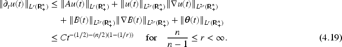
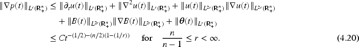
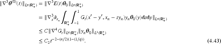
Proof of Theorem 1.4. We now establish the decay of

‖ \nabla^{2} u (t) ‖_{L^{\infty} (R_{+}^{n})}

and

\nabla^{2} B (t) ‖_{L^{\infty} (R_{+}^{n})}

Let $(u, B, θ)$ be the solution to problem (1.1), and assume $0 < η < 1$ . Then, for $1 < r < \infty$

\begin{aligned} ‖ x_{n}^{- η} u (t) \cdot \nabla B (t) ‖_{L^{r} (R_{+}^{n})} \leq C (‖ u (t) ‖_{L^{2 r} (R_{+}^{n})}^{2} + ‖ \nabla u (t) ‖_{L^{2 r} (R_{+}^{n})}^{2} + ‖ \nabla B (t) ‖_{L^{2 r} (R_{+}^{n})}^{2}) . \end{aligned}

(4.25)

Similarly, it holds that

\begin{aligned} ‖ x_{n}^{- η} θ (t) ‖_{L^{r} (R_{+}^{n})} \leq ‖ θ (t) ‖_{L^{r} (R_{+}^{n})} + ‖ \nabla θ (t) ‖_{L^{r} (R_{+}^{n})} . \end{aligned}

(4.26)

Liu and Yu (2015) contain the proof of (4.25). For readers’ convenience, we briefly provide the proof of (4.26). Note that for

t > 0

θ (x^{'}, 0, t) = 0

\begin{aligned} ‖ x_{n}^{- η} θ (t) ‖_{L^{r} (R^{n - 1} \times (0, 1))}^{r} & \leq \int_{0}^{1} \int_{R^{n - 1}} x_{n}^{- η r} | θ (x^{'}, x_{n}, t) - θ (x^{'}, 0, t) |^{r} d x^{'} d x_{n} \\ \leq \int_{0}^{1} \int_{R^{n - 1}} x_{n}^{r - 1 - η r} \int_{0}^{x_{n}} | \partial_{n} θ (x^{'}, z_{n}, t) |^{r} d z_{n} d x^{'} d x_{n} \\ \leq \int_{R^{n - 1}} \int_{0}^{1} | \partial_{n} θ (x^{'}, z_{n}, t) |^{r} d z_{n} d x_{n} \\ \leq ‖ \nabla θ (t) ‖_{L^{r} (R_{+}^{n})}^{r} . \end{aligned}

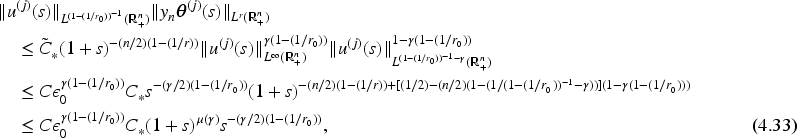
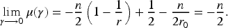
In order to estimate

‖ \nabla^{2} u (t) ‖_{L^{\infty} (R_{+}^{n})}

, Lemma 2.8 and an estimate for

‖ x_{n} θ (t) ‖_{L^{r} (R_{+}^{n})}

, with

r \in (1, \infty)

, are required. Nevertheless, as the bound of

‖ x_{n} θ (t) ‖_{L^{r} (R_{+}^{n})}

remains unobtained, we proof it by inductive hypothesis.

\begin{aligned} x_{n} E (t) θ_{0} (x) & = x_{n} \int_{R_{+}^{n}} [G_{t} (x^{'} - y^{'}, x_{n} - y_{n}) - G_{t} (x^{'} - y^{'}, x_{n} + y_{n})] θ_{0} (y) d y \\ = x_{n} \int_{R_{+}^{n}} \int_{- 1}^{1} \partial_{x_{n}} G_{t} (x^{'} - y^{'}, x_{n} - s y_{n}) (- y_{n}) θ_{0} (y) d s d y \\ = \int_{- 1}^{1} \int_{R_{+}^{n}} (x_{n} - s y_{n}) \partial_{x_{n}} G_{t} (x^{'} - y^{'}, x_{n} - s y_{n}) (- y_{n}) θ_{0} (y) d y d s \\ + \int_{- 1}^{1} \int_{R_{+}^{n}} \partial_{x_{n}} G_{t} (x^{'} - y^{'}, x_{n} - s y_{n}) s y_{n} (- y_{n}) θ_{0} (y) d y d s . \end{aligned}

(4.27)

y_{n} c, y_{n}^{2} c \in L^{1} (R_{+}^{n})

, it follows for

1 < r < \infty

and

t > 0

that

\begin{aligned} ‖ x_{n} θ^{(0)} (t) ‖_{L^{r} (R_{+}^{n})} & = ‖ x_{n} E (t) θ_{0} ‖_{L^{r} (R_{+}^{n})} \\ \leq C (‖ x_{n} \partial_{n} G_{t} ‖_{L^{r} (R^{n})} ‖ y_{n} θ_{0} ‖_{L^{1} (R_{+}^{n})} + ‖ \partial_{n} G_{t} ‖_{L^{r} (R^{n})} ‖ y_{n}^{2} θ_{0} ‖_{L^{1} (R_{+}^{n})}) \\ \leq {\tilde{C}}_{0} t^{- (n / 2) (1 - (1 / r))} . \end{aligned}

(4.28)

Assume there exists

j \geq 0

, such that

‖ x_{n} θ^{(j)} (t) ‖_{L^{r} (R_{+}^{n})} \leq C_{* *} t^{- (n / 2) (1 - (1 / r))},

where

{\tilde{C}}_{*} \geq {\tilde{C}}_{0}

. Let

(1 / r_{0}) = (1 / n) + (1 / r)

1 < r < \infty

, we have

\begin{aligned} ‖ x_{n} θ^{(j + 1)} (t) ‖_{L^{r} (R_{+}^{n})} \\ \leq ‖ x_{n} E (t) θ_{0} ‖_{L^{r} (R_{+}^{n})} + C \int_{0}^{t / 2} ‖ x_{n} \nabla G_{t - s} ‖_{L^{r} (R^{n})} ‖ u^{(j)} (s) ‖_{L^{2} (R_{+}^{n})} ‖ θ^{(j)} (s) ‖_{L^{r} (R^{n})} d s \\ + C \int_{0}^{t / 2} ‖ \nabla G_{t - s} ‖_{L^{r_{0}} (R^{n})} ‖ u^{(j)} (s) ‖_{L^{(1 - (1 / r_{0}))^{- 1}} (R_{+}^{n})} ‖ y_{n} θ^{(j)} (s) ‖_{L^{r} (R_{+}^{n})} d s \\ + C \int_{t / 2}^{t} ‖ x_{n} \nabla G_{t - s} ‖_{L^{1} (R^{n})} ‖ u^{(j)} (s) ‖_{L^{\infty} (R_{+}^{n})} ‖ θ^{(j)} (s) ‖_{L^{r} (R_{+}^{n})} d s \\ + C \int_{t / 2}^{t} ‖ \nabla G_{t - s} ‖_{L^{1} (R^{n})} ‖ u^{(j)} (s) ‖_{L^{\infty} (R_{+}^{n})} ‖ y_{n} θ^{(j)} (s) ‖_{L^{r} (R_{+}^{n})} d s \\ = J_{1} (t) + J_{2} (t) + J_{3} (t) + J_{4} (t) . \end{aligned}

(4.29)

Using Theorems 1.2 and 1.3, we obtain

\begin{aligned} J_{1} (t) & \leq C t^{- (n / 2) (1 - (1 / r))} + C \int_{0}^{t / 2} (t - s)^{- (n / 2) (1 - (1 / r))} (1 + s)^{(1 / 2) - (n / 4) - ((n + 2) / 4)} d s \\ \leq C t^{- (n / 2) (1 - (1 / r))} + C t^{- (n / 2) (1 - (1 / r))} \int_{0}^{\infty} (1 + s)^{- (n / 2)} d s \\ \leq C t^{- (n / 2) (1 - (1 / r))}, \end{aligned}

(4.30)

\begin{aligned} J_{3} (t) & \leq C ϵ_{0} \int_{t / 2}^{t} s^{- (1 / 2) - (n / 2) (1 - (1 / r))} d s \leq C t^{- (n / 2) (1 - (1 / r))} \end{aligned}

(4.31)

and

\begin{aligned} J_{4} (t) \leq C ϵ_{0} C_{*} \int_{t / 2}^{t} s^{- (1 / 2) - (1 / 2) - (n / 2) (1 - (1 / r))} d s \leq C ϵ_{0} C_{*} t^{- (n / 2) (1 - (1 / r))} . \end{aligned}

(4.32)

Now, we estimate

J_{2} (t)

. Let

2 n / (n - 2) < r < \infty

. Choosing

(1 / r_{0}) = (1 / n) + (1 / r)

, we have for

0 < γ < (1 - (1 / γ_{0}))^{- 1} - (n / (n - 1))

and

s > 0

\begin{aligned} ‖ u^{(j)} (s) ‖_{L^{(1 - (1 / r_{0}))^{- 1}} (R_{+}^{n})} ‖ y_{n} θ^{(j)} (s) ‖_{L^{r} (R_{+}^{n})} \\ \leq {\tilde{C}}_{*} (1 + s)^{- (n / 2) (1 - (1 / r))} ‖ u^{(j)} (s) ‖_{L^{\infty} (R_{+}^{n})}^{γ (1 - (1 / r_{0}))} ‖ u^{(j)} (s) ‖_{L^{(1 - (1 / r_{0}))^{- 1} - γ} (R_{+}^{n})}^{1 - γ (1 - (1 / r_{0}))} \\ \leq C ϵ_{0}^{γ (1 - (1 / r_{0}))} C_{*} s^{- (γ / 2) (1 - (1 / r_{0}))} (1 + s)^{- (n / 2) (1 - (1 / r)) + [(1 / 2) - (n / 2) (1 - (1 / (1 - (1 / r_{0}))^{- 1} - γ))] (1 - γ (1 - (1 / r_{0})))} \\ \leq C ϵ_{0}^{γ (1 - (1 / r_{0}))} C_{*} (1 + s)^{μ (γ)} s^{- (γ / 2) (1 - (1 / r_{0}))}, \end{aligned}

(4.33)

where

μ (γ) = - (n / 2) (1 - (1 / r)) + [(1 / 2) - (n / 2) (1 - (1 / (1 - (1 / r_{0}))^{- 1} - γ))] (1 - γ (1 - (1 / r_{0})))

. Note that

lim_{γ ⟶ 0} μ (γ) = - \frac{n}{2} (1 - \frac{1}{r}) + \frac{1}{2} - \frac{n}{2 r_{0}} = - \frac{n}{2} .

Thus, there exists

γ \in (0, (1 - (1 / γ_{0}))^{- 1} - (n / (n - 1)))

such that

1 + μ (γ) < 0 and 1 - (γ / 2) (1 - (1 / r_{0})) > 0.

Let $t > 2$ , then

\int_{0}^{t / 2} (1 + s)^{μ (γ)} s^{- (γ / 2) (1 - (1 / r_{0}))} d s \leq \int_{0}^{1} s^{- (γ / 2) (1 - (1 / r_{0}))} d s + \int_{1}^{t / 2} (1 + s)^{μ (γ)} d s \leq C .

0 < t \leq 2

\int_{0}^{t / 2} (1 + s)^{μ (γ)} s^{- (γ / 2) (1 - (1 / r_{0}))} d s \leq \int_{0}^{1} s^{- (γ / 2) (1 - (1 / r_{0}))} d s \leq C .

Then, for any

t > 0

, we have

\int_{0}^{t / 2} (1 + s)^{μ (γ)} s^{- (γ / 2) (1 - (1 / r_{0}))} d s \leq C .

Therefore, we obtain

\begin{aligned} \begin{aligned} J_{2} (t) & \leq C ϵ_{0}^{γ (1 - (1 / r_{0}))} C_{* *} \int_{0}^{t / 2} (t - s)^{- (1 / 2) - (n / 2) (1 - (1 / r_{0}))} (1 + s)^{μ (γ)} s^{- (γ / 2) (1 - (1 / r_{0}))} d s \\ \leq C ϵ_{0}^{γ (1 - (1 / n) - (1 / r))} C_{*} t^{- (n / 2) (1 - (1 / r))} . \end{aligned} \end{aligned}

(4.34)

Thus, we obtain

\begin{aligned} ‖ x_{n} θ^{(j + 1)} (t) ‖_{L^{r} (R_{+}^{n})} \leq {\tilde{C}}_{1} t^{- (n / 2) (1 - (1 / r))} + {\tilde{C}}_{1} (ϵ_{0} + ϵ_{0}^{γ (1 - (1 / n) - (1 / γ))}) C_{*} t^{- (n / 2) (1 - (1 / r))} . \end{aligned}

(4.35)

Take

ϵ_{0} > 0

suitably small such that

{\tilde{C}}_{1} (ϵ_{0} + ϵ_{0}^{γ (1 - (1 / n) - (1 / γ))}) \leq (1 / 2), and {\tilde{C}}_{*} = {\tilde{C}}_{0} + 2 {\tilde{C}}_{1}

, we have for any

t > 0

and

2 n / (n - 2) < r < \infty

\begin{aligned} ‖ x_{n} θ^{(j + 1)} (t) ‖_{L^{r} (R_{+}^{n})} \leq {\tilde{C}}_{*} t^{- (n / 2) (1 - (1 / r))} . \end{aligned}

(4.36)

From the estimates derived above, it follows that

sup_{j \geq 0} ‖ x_{n} θ^{(j + 1)} (t) ‖_{L^{r} (R_{+}^{n})} \leq {\tilde{C}}_{*} t^{- (n / 2) (1 - (1 / r))} .

Using the weak convergence procedure, we obtain for

2 n / (n - 2) < r < \infty

and any

t > 0

\begin{aligned} ‖ x_{n} θ (t) ‖_{L^{r} (R_{+}^{n})} \leq {\tilde{C}}_{*} t^{- (n / 2) (1 - (1 / r))} . \end{aligned}

(4.37)

Combining Lemmas 2.4 and 2.5, we have

\begin{aligned} ‖ \nabla^{2} u (t) ‖_{L^{\infty} (R_{+}^{n})} + ‖ \nabla^{2} B (t) ‖_{L^{\infty} (R_{+}^{n})} \\ \leq {‖ \nabla^{2} e^{- (t / 2) A} u (\frac{t}{2}) ‖}_{L^{\infty} (R_{+}^{n})} + {‖ \nabla^{2} e^{- (t / 2) A} B (\frac{t}{2}) ‖}_{L^{\infty} (R_{+}^{n})} \\ + \int_{t / 2}^{t} ‖ \nabla^{2} e^{- (t - s) A} P (u (s) \cdot \nabla u (s) - B (s) \cdot \nabla B (s) - θ e_{n}) ‖_{L^{\infty} (R_{+}^{n})} d s \\ + \int_{t / 2}^{t} ‖ \nabla^{2} e^{- (t - s) A} P (u (s) \cdot \nabla B (s) - B (s) \cdot \nabla u (s)) ‖_{L^{\infty} (R_{+}^{n})} d s \\ \leq C t^{- 1 - (n / 2 r)} ({‖ u (\frac{t}{2}) ‖}_{L^{r} (R_{+}^{n})} + {‖ B (\frac{t}{2}) ‖}_{L^{r} (R_{+}^{n})}) \\ + C \int_{t / 2}^{t} (t - s)^{- (1 / 2) - (n / 2 r)} ‖ \nabla (P u (s) \cdot \nabla u (s) - P B (s) \cdot \nabla B (s) - P θ (s) e_{n}) ‖_{L^{r} (R_{+}^{n})} d s \\ + C \int_{t / 2}^{t} (t - s)^{- 1 + (η / 2) - (n / 2 r)} ‖ x_{n}^{- η} (P u (s) \cdot \nabla u (s) - P B (s) \cdot \nabla B (s) - P θ (s) e_{n}) ‖_{L^{r} (R_{+}^{n})} d s \\ + C \int_{t / 2}^{t} (t - s)^{- (1 / 2) - (n / 2 r)} ‖ \nabla (P u (s) \cdot \nabla B (s) - P B (s) \cdot \nabla u (s) ‖_{L^{r} (R_{+}^{n})} d s \\ + C \int_{t / 2}^{t} (t - s)^{- 1 + (η / 2) - (n / 2 r)} ‖ x_{n}^{- η} (P u (s) \cdot \nabla B (s) - P B (s) \cdot \nabla u (s) ‖_{L^{r} (R_{+}^{n})} d s \\ = T_{1} (t) + T_{2} (t) + T_{3} (t) + T_{4} (t) + T_{5} (t) . \end{aligned}

(4.38)

Now, we turn to estimate

T_{i}, i = 1, 2, 3, 4, 5

. By Lemmas 2.8, 2.9, 4.1, Theorem 1.3 and (4.37), we obtain for any

t > 0

and

2 n / (n - 2) < r < \infty

\begin{aligned} T_{1} & \leq C t^{- ((n + 1) / 2)}, \end{aligned}

(4.39)

\begin{aligned} T_{2} & \leq C \int_{t / 2}^{t} (t - s)^{- (1 / 2) - (n / 2 r)} (‖ \nabla (u (s) \cdot \nabla u (s)) ‖_{L^{r} (R_{+}^{n})} + {‖ \nabla (\sum_{i, j = 1}^{n} \nabla N \partial_{i} \partial_{j} (u_{i} u_{j}) (s)) ‖}_{L^{r} (R_{+}^{n})} \\ + ‖ \nabla (B (s) \cdot \nabla B (s)) ‖_{L^{r} (R_{+}^{n})} + {‖ \nabla (\sum_{i, j = 1}^{n} \nabla N \partial_{i} \partial_{j} (B_{i} B_{j}) (s)) ‖}_{L^{r} (R_{+}^{n})} \\ + ‖ \nabla θ (s) ‖_{L^{r} (R_{+}^{n})} + ‖ \nabla^{2} N div (θ (s) e_{n}) ‖_{L^{r} (R_{+}^{n})}) d s \\ \leq C \int_{t / 2}^{t} (t - s)^{- (1 / 2) - (n / 2 r)} ({‖ u (s) ‖}_{L^{2 r} (R_{+}^{n})}^{2} + ‖ \nabla u (s) ‖_{L^{2 r} (R_{+}^{n})}^{2} + ‖ \nabla^{2} u (s) ‖_{L^{2 r} (R_{+}^{n})}^{2} \\ + {‖ B (s) ‖}_{L^{2 r} (R_{+}^{n})}^{2} + ‖ \nabla B (s) ‖_{L^{2 r} (R_{+}^{n})}^{2} + ‖ \nabla^{2} B (s) ‖_{L^{2 r} (R_{+}^{n})}^{2} + {‖ θ (s) ‖}_{L^{r} (R_{+}^{n})} \\ + {‖ \nabla θ (s) ‖}_{L^{r} (R_{+}^{n})} + ‖ \nabla^{2} θ (s) ‖_{L^{r} (R_{+}^{n})}) d s \\ \leq C \int_{t / 2}^{t} (t - s)^{- (1 / 2) - (n / 2 r)} (s^{1 - n (1 - (1 / 2 r))} + s^{- (1 / 2) - (n / 2) (1 - (1 / r))}) d s \\ \leq C t^{- (n / 2)} (1 + t^{- ((n - 3) / 2)}) . \end{aligned}

(4.40)

Moreover, for

max {n / η, 2 n / (n - 2)} < r < \infty

\begin{aligned} T_{3} & \leq C \int_{t / 2}^{t} (t - s)^{- 1 + (η / 2) - (η / 2 r)} (‖ x_{n}^{- η} u (s) \cdot \nabla u (s) ‖_{L^{r} (R_{+}^{n})} + {‖ \sum_{i, j = 1}^{n} x_{n}^{- η} \nabla N \partial_{i} \partial_{j} (u_{i} u_{j}) (s) ‖}_{L^{r} (R_{+}^{n})} \\ + ‖ x_{n}^{- η} B (s) \cdot \nabla B (s) ‖_{L^{r} (R_{+}^{n})} + {‖ \sum_{i, j = 1}^{n} x_{n}^{- η} \nabla N \partial_{i} \partial_{j} (B_{i} B_{j}) (s) ‖}_{L^{r} (R_{+}^{n})} \\ + ‖ x_{n}^{- η} θ (s) ‖_{L^{r} (R_{+}^{n})} + ‖ x_{n}^{- η} \nabla N div (θ (s) e_{n}) ‖_{L^{r} (R_{+}^{n})}) d s \\ \leq C \int_{t / 2}^{t} (t - s)^{- (1 / 2) - (n / 2 r)} ({‖ u (s) ‖}_{L^{2 r} (R_{+}^{n})}^{2} + ‖ \nabla u (s) ‖_{L^{2 r} (R_{+}^{n})}^{2} + {‖ B (s) ‖}_{L^{2 r} (R_{+}^{n})}^{2} + ‖ \nabla B (s) ‖_{L^{2 r} (R_{+}^{n})}^{2} \\ + {‖ θ (s) ‖}_{L^{r} (R_{+}^{n})} + {‖ \nabla θ (s) ‖}_{L^{r} (R_{+}^{n})} + ‖ y_{n} θ (s) ‖_{L^{r} (R_{+}^{n})}) d s \\ \leq C \int_{t / 2}^{t} (t - s)^{- 1 + (η / 2) - (n / 2 r)} (s^{1 - n (1 - (1 / 2 r))} + s^{- (n / 2) (1 - (1 / r))}) d s \\ \leq C t^{- (n / 2) + (η / 2)} (1 + t^{- ((n - 2) / 2)}) . \end{aligned}

(4.41)

Similarly, we have

T_{4} \leq C \int_{t / 2}^{t} (t - s)^{- (1 / 2) - (n / 2 r)} s^{1 - n (1 - (1 / 2 r))} d s \leq C t^{- n + (3 / 2)}

and

T_{5} \leq C \int_{t / 2}^{t} (t - s)^{- 1 + (η / 2) - (n / 2 r)} s^{1 - n (1 - (1 / 2 r))} d s \leq C t^{- n + (η / 2) + 1} .

From the estimates derived above, we have for

max {n / η, 2 n / (n - 2)} < r < \infty

\begin{aligned} ‖ \nabla^{2} u (t) ‖_{L^{\infty} (R_{+}^{n})} + ‖ \nabla^{2} B (t) ‖_{L^{\infty} (R_{+}^{n})} \leq C t^{- (n / 2) + (η / 2)} . \end{aligned}

(4.42)

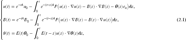
Now, we establish the decay of $‖ \nabla^{3} θ (t) ‖_{L^{r} (R_{+}^{n})}$ by induction as before. We can easily verify that for $1 \leq q \leq \infty$ and $t > 0$

\begin{aligned} ‖ \nabla^{3} θ^{(0)} (t) ‖_{L^{q} (R_{+}^{n})} & = ‖ \nabla^{3} E (t) θ_{0} ‖_{L^{q} (R_{+}^{n})} \\ = ‖ \nabla_{x}^{3} \partial_{x_{n}} \int_{R_{+}^{n}} \int_{- 1}^{1} G_{t} (x^{'} - y^{'}, x_{n} - s y_{n}) y_{n} θ_{0} (y) d s d y ‖_{L^{q} (R_{+}^{n})} \\ \leq C ‖ \nabla^{4} G_{t} ‖_{L^{q} (R_{+}^{n})} ‖ y_{n} θ_{0} ‖_{L^{1} (R_{+}^{n})} \\ \leq C_{2} t^{- 2 - (n / 2) (1 - (1 / q))} . \end{aligned}

(4.43)

Assume that

\begin{aligned} ‖ \nabla^{3} θ^{(j)} (t) ‖_{L^{q} (R_{+}^{n})} \leq C_{* *} t^{- 2 - (n / 2) (1 - (1 / q))} . \end{aligned}

(4.44)

To continue our analysis, we conclude some fundamental properties of $E (t) and F (t)$ :

\begin{aligned} \partial_{m}^{k} [E (t) g] = E (t) \partial_{m}^{k} g a n d \partial_{m}^{k} [F (t) g] = F (t) \partial_{m}^{k} g, \forall 1 \leq m \leq n - 1, k = 1, 2, \dots, \end{aligned}

(4.45)

\begin{aligned} \partial_{n} [E (t) f] = F (t) \partial_{n} f f o r a n y f |_{\partial R_{+}^{n}} = 0, \end{aligned}

(4.46)

\begin{aligned} \partial_{n} [F (t) g] = E (t) \partial_{n} g . \end{aligned}

(4.47)

As recalled earlier, for any

t > 0

and

1 \leq q \leq \infty

, then

θ^{(j + 1)} (t) = E (\frac{t}{2}) θ^{(j + 1)} (\frac{t}{2}) - \int_{t / 2}^{t} E (t - s) u^{(j)} (s) \cdot \nabla θ^{(j)} (s) d s

holds.

Let $1 \leq q < \infty$ , using (3.44)–(3.48) and Theorems 1.2 and 1.3, we obtain for any $t \geq 1$

\begin{aligned} ‖ \nabla^{3} θ^{(j + 1)} (t) ‖_{L^{q} (R_{+}^{n})} \\ \leq {‖ \nabla^{3} E (\frac{t}{2}) θ^{(j + 1)} (\frac{t}{2}) ‖}_{L^{q} (R_{+}^{n})} + 2 \int_{t / 2}^{t} ‖ \nabla G_{t - s} ‖_{L^{1} (R^{n})} ‖ \nabla^{2} (u^{(j)} (s) \cdot \nabla θ^{(j)} (s)) ‖_{L^{q} (R_{+}^{n})} d s \\ \leq C t^{- (3 / 2)} {‖ θ^{(j + 1)} (\frac{t}{2}) ‖}_{L^{q} (R_{+}^{n})} + C \int_{t / 2}^{t} (t - s)^{- (1 / 2)} ‖ \nabla^{2} u^{(j)} (s) ‖_{L^{2 q} (R_{+}^{n})} ‖ \nabla θ^{(j)} (s) ‖_{L^{2 q} (R_{+}^{n})} d s \\ + C \int_{t / 2}^{t} (t - s)^{- (1 / 2)} ‖ \nabla u^{(j)} (s) ‖_{L^{\infty} (R_{+}^{n})} ‖ \nabla^{2} θ^{(j)} (s) ‖_{L^{q} (R_{+}^{n})} d s \\ + C \int_{t / 2}^{t} (t - s)^{- (1 / 2)} ‖ u^{(j)} (s) ‖_{L^{\infty} (R_{+}^{n})} ‖ \nabla^{3} θ^{(j)} (s) ‖_{L^{q} (R_{+}^{n})} d s \\ \leq C t^{- 2 - (n / 2) (1 - (1 / q))} + C t^{- (1 / 2) - (n / 2) (1 - (1 / 2 q))} \int_{t / 2}^{t} (t - s)^{- (1 / 2)} s^{- 1 - (n / 2) (1 - (1 / 2 q))} d s \\ + C \int_{t / 2}^{t} (t - s)^{- (1 / 2)} s^{- (n / 2) - (3 / 2) - (n / 2) (1 - (1 / q))} d s + C ϵ_{0} C_{* *} \int_{t / 2}^{t} (t - s)^{- (1 / 2)} s^{- (1 / 2) - 2 - (n / 2) (1 - (1 / q))} d s \\ \leq C t^{- 2 - (n / 2) (1 - (1 / q))} + C t^{- ((n + 2) / 2) - (n / 2) (1 - (1 / q))} + C ϵ_{0} C_{* *} t^{- 2 - (n / 2) (1 - (1 / q))} \\ \leq {\tilde{C}}_{2} t^{- 2 - (n / 2) (1 - (1 / q))} + C ϵ_{0} C_{* *} t^{- 2 - (n / 2) (1 - (1 / q))} . \end{aligned}

(4.48)

Taking

C ϵ_{0} \leq (1 / 2)

C_{* *} = C_{2} + 2 {\tilde{C}}_{2}

, we conclude that

sup_{j \geq 0} ‖ \nabla^{3} θ^{(j)} (t) ‖_{L^{q} (R_{+}^{n})} \leq C_{* *} t^{- 2 - (n / 2) (1 - (1 / q))} .

By a standard weak convergence procedure, we get

\begin{aligned} ‖ \nabla^{3} θ (t) ‖_{L^{q} (R_{+}^{n})} \leq C t^{- 2 - (n / 2) (1 - (1 / q))} . \end{aligned}

(4.49)

When

q = \infty

, we have from (4.48) and taking

0 < ϵ < (n - 3) / 2

that

\begin{aligned} ‖ \nabla^{3} θ^{(j + 1)} (t) ‖_{L^{\infty} (R_{+}^{n})} & \leq C t^{- 2 - (n / 2)} + C t^{- (n / 2) + ϵ} \int_{t / 2}^{t} (t - s)^{- (1 / 2)} s^{- 1 - (n / 2)} d s \\ + C \int_{t / 2}^{t} (t - s)^{- (1 / 2)} s^{- (n / 2) - (3 / 2) - (n / 2)} d s \\ + C ϵ_{0} C_{* *} \int_{t / 2}^{t} (t - s)^{- (1 / 2)} s^{- (1 / 2) - 2 - (n / 2)} d s \\ \leq C t^{- 2 - (n / 2)} + C t^{- 2 - (n / 2) + ϵ - ((n - 3) / 2)} + C ϵ_{0} C_{* *} t^{- 2 - (n / 2)} \\ \leq {\begin{cases} \tilde{C} t^{- 2 - (n / 2) + ϵ} & if n = 3, \\ \tilde{C} t^{- 2 - (n / 2)} & if n > 3. \end{cases} \end{aligned}

(4.50)

Following a standard weak convergence argument, we get for

\tilde{C} > 0

and

t \geq 1

\begin{aligned} ‖ \nabla^{3} θ (t) ‖_{L^{\infty} (R_{+}^{n})} \leq {\begin{cases} \tilde{C} t^{- 2 - (n / 2) + ϵ} & if n = 3, \\ \tilde{C} t^{- 2 - (n / 2)} & if n > 3. \end{cases} \end{aligned}

(4.51)

Based on the estimates above, the proof of Theorem 1.4 is completed. □

Footnotes

ORCID iD

Yuzhu Wang

Funding

The authors disclosed receipt of the following financial support for the research, authorship, and/or publication of this article: This work is supported by the Program for Innovative Research Team (in Science and Technology) in the University of Henan Province (Grant No. 25IRTSTHN013).

Declaration of Conflicting Interests

The authors declared no potential conflicts of interest with respect to the research, authorship, and/or publication of this article.

Data Availability Statement

Data sharing is not applicable to this article as no data sets were generated or analyzed during the current study.

References

Abidi

Gui

G. L.

Zhang

(2011). On the decay and stability of global solutions to the 3D inhomogeneous Navier–Stokes equations. Communications on Pure and Applied Mathematics, 64, 832–881. 10.1002/cpa.20351

Abidi

Hmidi

Keraani

(2011). On the global regularity of axisymmetric Navier–Stokes–Boussinesq system. Discrete and Continuous Dynamical Systems, 29, 737–756. 10.3934/dcds.2011.29.737

Bae

H. O.

Choe

H. J.

(2001). Decay rate for the incompressible flows in half spaces. Mathematische Zeitschrift, 238, 799–816. 10.1007/s002090100276

Borchers

Miyakawa

(1988).

L^{2}

decay for the Navier–Stokes flow in half spaces. Mathematische Annalen, 282, 139–155. 10.1007/BF01457017

Brandolese

(2004). Asymptotic behavior of the energy and pointwise estimates for solutions to the Navier–Stokes equations. Revista Matematica Iberoamericana, 20, 223–256. 10.4171/rmi/387

Brandolese

Schonbek

M. E.

(2012). Large time decay and growth for solutions of a viscous Boussinesq system. Transactions of the American Mathematical Society, 364, 5057–5090. 10.1090/S0002-9947-2012-05432-8

Cannone

Planchon

Schonbek

M. E.

(2000). Strong solutions to the incompressible Navier–Stokes equations in the half-space. Communications in Partial Differential Equations, 25, 903–924. 10.1080/03605300008821536

Chen

Wang

(2024). The

L^{1}

-asymptotic behavior of strong solutions to the incompressible magneto-hydrodynamic equations in half-spaces. Applied Mathematics Letters, 150, Article 108966. 10.1016/j.aml.2023.108966

Fan

Sun

J. Z.

Tang

(2019). Uniform global strong solutions of the 2D density-dependent incompressible magnetic Bénard problem in a bounded domain. Computers & Mathematics with Applications (Oxford, England), 77, 494–500. 10.1016/j.camwa.2018.09.052

10.

Fujigaki

Miyakawa

(2001). Asymptotic profiles of non stationary incompressible Navier–Stokes flows in the half-space. Methods and Applications of Analysis, 8, 121–158. 10.4310/MAA.2001.v8.n1.a6

11.

Han

(2010). Asymptotic behavior for the Stokes flow and Navier–Stokes equations in half spaces. Journal of Differential Equations, 249, 1817–1852. 10.1016/j.jde.2010.05.021

12.

Han

(2011). Decay results of solutions to the incompressible Navier–Stokes flows in a half space. Journal of Differential Equations, 250, 3937–3959. 10.1016/j.jde.2010.11.018

13.

Han

(2012). Weighted decay properties for the incompressible Stokes flow and Navier–Stokes equations in a half space. Journal of Differential Equations, 253, 1744–1778. 10.1016/j.jde.2012.06.007

14.

Han

(2022). Decay properties for the incompressible Navier–Stokes flows in a half space. Proceedings of the Royal Society of Edinburgh Section A, 152, 1509–1532. 10.1017/prm.2021.63

15.

Han

(2024).

L^{1}

-decay of higher-order norms of solutions to the Navier–Stokes equations in the upper-half space. Mathematische Zeitschrift, 308, Article 23. 10.1007/s00209-024-03578-6

16.

Han

Schonbek

M. E.

(2014). Large time decay properties of solutions to a viscous Boussinesq system in a half space. Advances in Differential Equations, 19, 87–132. 10.57262/ade/1384278133

17.

Xin

(2005). On the regularity of weak solutions to the magnetohydrodynamic equations. Journal of Differential Equations, 213, 235–254. 10.1016/j.jde.2004.07.002

18.

Hmidi

Rousset

(2010). Global well-posedness for the Navier–Stokes–Boussinesq system with axisymmetric data. Annales de l’Institut Henri Poincaré C, Analyse Non Linéaire, 27, 1227–1246. 10.1016/j.anihpc.2010.06.001

19.

Huang

(2023). Stability and exponential decay of the magnetic Bénard system with horizontal dissipation. Journal of Mathematical Analysis and Applications, 519, Article 126767. 10.1016/j.jmaa.2022.126767

20.

Kato

(1984). Strong

L^{p}

-solutions of the Navier–Stokes equation in

R^{m}

, with applications to weak solutions. Mathematische Zeitschrift, 187, 471–480. 10.1007/BF01174182

21.

Kozono

Ogawa

(1992). Some

L^{p}

estimate for the exterior Stokes flow and an application to the nonstationary Navier–Stokes equations. Indiana University Mathematics Journal, 41, 789–808. 10.1512/iumj.1992.41.41041

22.

Lemarié

P.-G.

(2002). Recent developments in the Navier–Stokes problem. CRC Press.

23.

Leray

(1934). Sur le mouvement d’un liquide visqueux emplissant l’espace. Acta Mathematica, 63, 193–248. 10.1007/BF02547354

24.

Wang

(2020). Uniform regularity estimates of solutions to three dimensional incompressible magnetic Bénard equations with Navier-slip type boundary conditions in half space. Nonlinear Analysis, 199, Article 111932. 10.1016/j.na.2020.111932

25.

Tan

(2022). Global existence and decay estimates of solutions to the MHD–Boussinesq system with stratification effects. Nonlinearity, 35, 6067–6097. 10.1088/1361-6544/ac93e0

26.

(2024). Large time behavior of the solutions to 3D incompressible MHD system with horizontal dissipation or horizontal magnetic diffusion. Calculus of Variations and Partial Differential Equations, 63, Article 43. 10.1007/s00526-023-02647-8

27.

Liu

(2019). Asymptotic behavior of solutions to the nonstationary magneto-hydrodynamic equations. Nonlinear Analysis, 185, 29–48. 10.1016/j.na.2019.02.030

28.

Liu

(2020). Algebraic decay of weak solutions to 3D Navier–Stokes equations in general unbounded domains. Journal of Mathematical Analysis and Applications, 491, Article 124300. 10.1016/j.jmaa.2020.124300

29.

Liu

Han

(2024). Long time behavior for the two-dimensional magnetohydrodynamic flows in a general domain. Journal of Mathematical Physics, 65, Article 111501. 10.1063/5.0223634

30.

Liu

(2015). Large time behavior for the incompressible magnetohydrodynamic equations in half-spaces. Mathematical Methods in the Applied Sciences, 38, 2376–2388. 10.1002/mma.3227

31.

Luo

Sun

(2025). Global solution of 3D MHD–Boussinesq system with mixed partial dissipation and thermal damping. Discrete and Continuous Dynamical Systems—Series B, 30, 1029–1049. 10.3934/dcdsb.2024118

32.

Pan

(2022). Global regularity of solutions for the 3D non-resistive and non-diffusive MHD–Boussinesq system with axisymmetric data. Acta Applicandae Mathematicae, 180, Article 6. 10.1007/s10440-022-00508-8

33.

Regmi

Sharma

(2019). Regularity criteria on the 2D anisotropic magnetic Bénard equations. Journal of Mathematical Study, 52, 60–74. 10.4208/jms.v52n1.19.06

34.

Rionero

(1998). On the magnetic Bénard problem. Rendiconti del Circolo Matematico di Palermo, 1998(2 Suppl), 419–426.

35.

Schonbek

M. E.

(1992). Asymptotic behavior of solutions to the three-dimensional Navier–Stokes equations. Indiana University Mathematics Journal, 41, 809–823. 10.1512/iumj.1992.41.41042

36.

Schonbek

M. E.

(1995). The Fourier splitting method. In Advances in geometric analysis and continuum mechanics (pp. 269–274). International Press.

37.

Schonbek

M. E.

Wiegner

(1996). On the decay of higher-order norms of the solutions of Navier–Stokes equations. Proceedings of the Royal Society of Edinburgh Section A, 126, 677–685. 10.1017/S0308210500022976

Time Decay Estimates of Solutions to the Magnetic Bénard System in a Half-Space

Abstract

Keywords

1. Introduction and Main Results

Lemma 2.5 Han, 2012

Lemma 2.6 Brandolese, 2004

Lemma 2.7 Borchers & Miyakawa, 1988

Lemma 2.8 Han, 2010, 2012

Lemma 2.9 Han, 2011; Liu, 2019

3. Decay Rates of Weak and Strong Solutions

3.1. L 2 -Decay of Weak Solutions

Footnotes

ORCID iD

Funding

Declaration of Conflicting Interests

Data Availability Statement

References

3.1. $L^{2}$ -Decay of Weak Solutions