Perceived Average Orientation Reflects Effective Gist of the Surface

Abstract

The human ability to represent ensemble visual information, such as average orientation and size, has been suggested as the foundation of gist perception. To effectively summarize different groups of objects into the gist of a scene, observers should form ensembles separately for different groups, even when objects have similar visual features across groups. We hypothesized that the visual system utilizes perceptual groups characterized by spatial configuration and represents separate ensembles for different groups. Therefore, participants could not integrate ensembles of different perceptual groups on a task basis. We asked participants to determine the average orientation of visual elements comprising a surface with a contour situated inside. Although participants were asked to estimate the average orientation of all the elements, they ignored orientation signals embedded in the contour. This constraint may help the visual system to keep the visual features of occluding objects separate from those of the occluded objects.

Keywords

average orientation diffusion model contour integration gist perception spatial configuration open data open materials

People extract the gist of a complex visual scene at a glance, and gist information can help them to recognize objects in a scene by ruling out improper alternatives for the targeted objects (Wolfe, Võ, Evans, & Greene, 2011). In a crime scene, for example, a red blob might appear to be a blood spill but is actually an apple in an orchard. Researchers have suggested that the ability to represent ensemble visual information is the foundation of gist perception (Alvarez, 2011). People have shown the ability to estimate summary information from various visual properties, including average orientation (Dakin & Watt, 1997; Parkes, Lund, Angelucci, Solomon, & Morgan, 2001), average size (Ariely, 2001; Chong & Treisman, 2003), summed area (Lee, Baek, & Chong, 2016), numerosity (Burr & Ross, 2008), and centroid location (Alvarez & Oliva, 2008). This ability enables people to quickly judge a complex scene crowded with a vast number of objects. One example might be a farmer evaluating the quantity of apples on a tree without counting each of them. Because irrelevant stimuli, green leaves, are distinct from the red apples in the color space, the proportion of red against green may be taken as an estimate of the quantity of apples. When objects are distinct in a single feature space, categorization is a matter of allocating them to distributions with distinct averages in that space (Fig. 1a; Utochkin, 2015). When different objects share similar features, however, it becomes difficult to categorize them. Imagine you are trying to distinguish limes among green leaves. Instead of relying on color, you may want to consider the spatial arrangement of limes in the scene. To deal with a complex visual scene in which objects share similar features, the brain must create ensemble representations that reflect the arrangement of the objects.

Fig. 1.

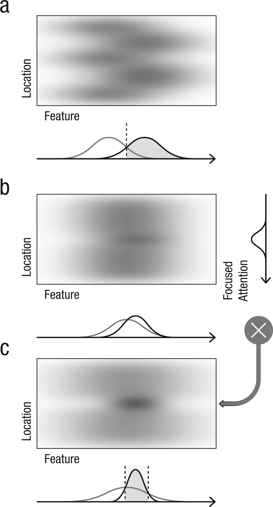
Examples of how observers discriminate feature distributions. Each panel depicts an imaginary map of responses to features over locations in one-dimensional space. Stronger responses are marked with darker shading. The line graphs below each map show a population response in the feature space. If visual features are evident from distributions with distinct peaks (gray and black lines in the graph in a), they can be discriminated on the basis of their feature values regardless of their spatial locations. However, if visual features are similar to one another (gray and black lines in the graph in b), it will be difficult to discriminate them on the basis of feature values. In this case, the visual system can consider the spatial locations of visual features. If focused attention (graph at the right side in b) is applied to a specific location, responses will increase at the focused location and decrease at the other locations (multiplicate modulation denoted by “X” in the gray circle between panels b and c). As a result, the response map in (b) will be transformed into the response map in (c). The feature distribution at the location of focused attention will be reshaped to the form of a narrow bell (black line in the graph in c) so that it can be discriminated from the other distribution (gray line in the graph in c).

One viable strategy to distinguish similar features of different objects is to modulate their responses in a feature space. When similar visual features of different elements are discriminable on the basis of their locations (Fig. 1b), the visual system can deploy different types of attention and reshape the response functions to different elements. Focusing attention on an object would narrow the response function, resulting in the selective response to the attended object feature (Carrasco, Ling, & Read, 2004; Ling & Carrasco, 2006). Distributing attention over multiple objects would form a broad population response, thereby representing the average feature at the cost of an individual object feature (Ariely, 2001; Chong & Treisman, 2003, 2005). By deploying focused and distributed attention to different perceptual groups at different spatial locations, the visual system can modulate and distinguish response functions from the different groups (Fig. 1c).

The same strategy can be applied when viewing a complex scene. In the visual periphery, object features are bound together and represented in summary because of visual crowding (Parkes et al., 2001). Although the summary features can contribute to a scene gist by themselves (Larson, Freeman, Ringer, & Loschky, 2014; Larson & Loschky, 2009), the visual system can separate crowded features of different perceptual groups by modulating responses to each group differently (Fig. 1c). For example, the salience of oriented visual elements can be boosted when those elements are aligned collinearly to form an extended contour (Field, Hayes, & Hess, 1993; Li & Gilbert, 2002; Polat & Sagi, 1994). This collinear alignment can be applied to crowded elements and can help observers distinguish perceptual groups among crowded elements. When the target stimulus is left out of a contour made of the other stimuli, it becomes easier to distinguish the target feature from the others (Livne & Sagi, 2007). It becomes difficult to distinguish the target feature if the target is part of a contour formed with the other stimuli (Mareschal, Morgan, & Solomon, 2010). Thus, the visual system can utilize spatial configuration to bind visual elements into perceptual groups while modulating responses to those groups differently.

We speculated that ensemble representation could take advantage of the perceptual groups characterized by spatial configurations. Once responses to different perceptual groups are modulated into distinct shapes, the visual system could form separate ensemble representations for each perceptual group. This speculation led us to predict that people could not blend ensembles of different perceptual groups because the responses to different groups conformed to distinctly shaped distributions. To test this prediction, we arranged oriented visual elements (Gabor patches) in such a way that some of the elements formed a contour inside a larger crowd of Gabor patches. Specifically, the experimental stimuli consisted of 60 oriented Gabor patches spread over a circular area. Among them, 9 Gabor patches were aligned on an imaginary line to form a contour. We hypothesized that participants would not blend the ensemble of the 9 contour Gabor patches to the ensemble of the other Gabor patches in the larger crowd. Thus, participants would ignore the orientations of the contour Gabor patches when asked to determine whether, on average, all 60 Gabor patches were tilted clockwise or counterclockwise. Participants were explicitly instructed to respond to the average orientation of the entire set of Gabor patches regardless of their configuration.

Method

Participants

Seven participants, including both authors, volunteered for the experiment. All participants had normal or corrected-to-normal vision, and the 5 who were not authors were naive to the purpose of the study. We determined the number of naive participants on the basis of the previous study on the integration of Gabor orientations (Dakin & Watt, 1997). All participants gave written consent, and every aspect of the study was carried out in accordance with the Yonsei University Institutional Review Board.

Apparatus and stimuli

Stimuli were generated using MATLAB (The MathWorks, Natick, MA) with the Psychophysics Toolbox Version 3 extension (Brainard, 1997; Kleiner, Brainard, & Pelli, 2007; Pelli, 1997) and were presented on a gamma-corrected CRT monitor (HP P1230; refresh rate: 85 Hz) in a dark room. Condensed but nonoverlapping placement of the stimuli was determined using custom functions in MATLAB (code is available at http://github.com/oakyoon/pretina). Each participant’s head was secured at 100 cm distance from the monitor using a head and chin rest.

The stimuli consisted of 60 Gabor patches spread over a circular area of 4.2° in diameter (Figs. 2a and 2b). The spatial frequency of the sinusoidal grating embedded in a Gabor was 8 cycles/degree, and the contrast was 84%. The standard deviation of the Gaussian envelope was 5.3 min arc. The background was uniform gray (39.31 cd/m²).

Fig. 2.

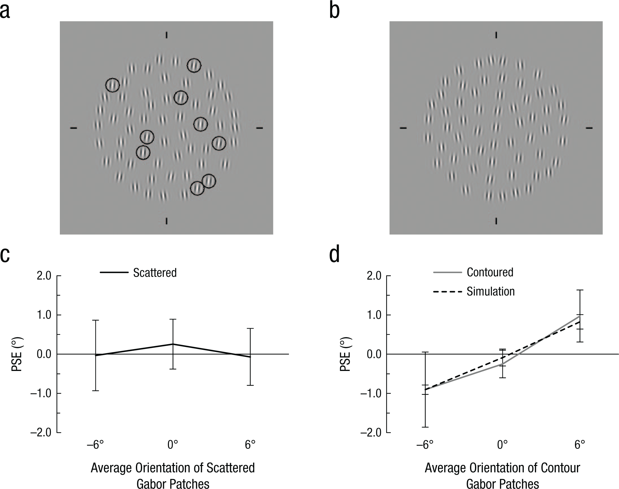
Example stimulus arrays from the scattered (a) and contoured (b) conditions and points of subject equality (PSEs) for each example (c and d, respectively). Stimulus arrays consisted of 60 Gabor patches, 9 of which were placed in a predetermined random arrangement throughout the array (scattered condition) or oriented in a vertical contour (contoured condition). The average orientation of Gabor patches is 0° (i.e., vertical meridian) in both examples. In (a), the prearranged Gabor patches are indicated by black circles (not present in the experiment), and they are tilted 6° clockwise on average. In (b), the prearranged Gabor patches are aligned on the imaginary line through the center of the circular area, forming a contour tilted 6° clockwise. Thus, the average orientation of the contour Gabor patches is 6° clockwise, and the average of the rest of the Gabor patches is about 1.06° counterclockwise, producing the total average of 0°. The graphs show the PSE in each condition, separately for each average orientation of the prearranged Gabor patches. Results are shown for the scattered and contoured conditions, as well as for simulated PSEs from the diffusion model. Note that a PSE shift toward the contour orientation leads to a response bias against the contour orientation. For instance, the PSE was around 1° with a 6° contour. Participants had a greater chance to respond “counterclockwise” in this condition, even if the average orientation was, say, 0.5°, because it was counterclockwise with reference to the PSE. Error bars indicate 95% confidence intervals.

Among the 60 Gabor patches, the location and orientation of 9 Gabor patches were prearranged depending on the experimental condition. In the scattered condition (Fig. 2a), the 9 prearranged patches were randomly scattered among the others, and they were tilted −6°, 0°, or 6° away from the vertical meridian on average. In the contoured condition (Fig. 2b), the prearranged Gabor patches were placed on an imaginary line tilted −6°, 0°, or 6° away from the vertical meridian, and they were tilted toward the same orientation as the imaginary line on average.

The average orientation of the entire crowd of 60 Gabor patches (including the prearranged Gabor patches) ran from −4.5° to 4.5° in steps of 1.5° (seven orientations total). The orientations of individual Gabor patches were sampled from a uniform probability distribution and then normalized to the designated average and standard deviation. The standard deviation in orientation of the prearranged Gabor patches was set to 1.86°, and that of the remaining 51 Gabor patches was set to 4.8°.

Design and procedure

The experimental conditions consisted of seven levels of average orientation (−4.5°, −3°, −1.5°, 0°, 1.5°, 3°, 4.5°), three levels of the prearranged Gabor orientation (−6°, 0°, 6°), and two types of configuration (scattered and contoured). Sixteen repetitions for each condition resulted in 336 trials per configuration. Every condition was tested in an intermixed fashion.

Participants started each trial by pressing the space bar. After a random delay of 600 to 1,000 ms, 60 Gabor patches were presented for 100 ms. Crosshairs were presented 1.37° outside the circular area throughout the whole experiment as a reference frame for the vertical and horizontal meridians. After the Gabor patches disappeared, participants reported whether the average orientation of the entire crowd was clockwise or counterclockwise. Self-paced breaks were given every 84 trials.

Participants completed 21 practice trials for each configuration, which resulted in 42 trials at the start of the experiment. In the practice trials, participants were encouraged to consider the entire crowd of Gabor patches to determine the average orientation, and auditory feedback was given to promote correct responses. When the average orientation was the same as the vertical meridian, feedback was given on a random basis. Feedback was not given in the experimental trials in order to prevent bias (Bauer, 2009).

Analysis

The proportion of “clockwise” responses to the seven average orientations was fitted to a cumulative Gaussian function using psignifit Version 3.0 (Fründ, Haenel, & Wichmann, 2011). A fitted function yielded four parameters: point of subjective equality (PSE), slope, lapse rate, and guessing rate. Among the parameters, PSE was a perceptual equivalent to the vertical meridian and thus provided an estimate of the response bias depending on the experimental manipulation (i.e., configuration and average orientation of the prearranged Gabor patches). The experiment produced six psychometric functions (2 configurations × 3 prearranged Gabor orientations).

Simulation

We hypothesized that participants would ignore orientation signals embedded in the contour when attention was distributed over the crowd of Gabor patches comprising the surrounding surface. To estimate the behavioral consequences of the strategies participants might employ, we simulated their responses using two different models. The models simulated behavioral responses to either all 60 Gabor patches or only 51 Gabor patches excluding the 9 contour Gabor patches.

First, we used a diffusion model (Ratcliff & Rouder, 1998) to simulate participants’ responses when orientation signals from all the Gabor patches equally contributed to the perceptual decision. The model accumulated perceptual evidence (i.e., orientation signal) to a certain threshold and determined its response. Perceptual evidence was sampled from Gaussian probability distributions centered at the orientation of each Gabor patch. The standard deviation of the Gaussian probability distribution produced perceptual noise. The model used in the current simulation is described as follows:

E (t) = E_{0} + \sum_{x = 1}^{t} e (x)

e (x) = \sum_{i = 1}^{n} X_{i}

X_{i} ~ N (θ_{i}, σ_{noise}^{2})

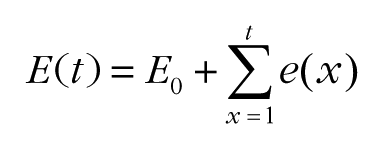
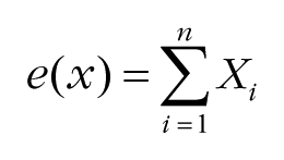
Perceptual evidence at a certain time point e(x) was accumulated over time. If the cumulative evidence E(t) reached the positive decision threshold (T_CW) first, the model responded “clockwise.” If the cumulative evidence reached the negative decision threshold (T_CCW) first, the model responded “counterclockwise.” Each Gabor patch contributed to the perceptual evidence e(x), and the amount of contribution X_i was randomly sampled from a Gaussian distribution whose mean was the Gabor orientation θ_i and whose standard deviation was σ_noise. The number of Gabor patches was denoted as n. We estimated model parameters for each participant using maximum likelihood estimation (Myung, 2003) to reproduce the behavioral data in the scattered condition. The noise standard deviation σ_noise, bias E₀, and positive decision threshold T_CW were estimated, and the negative decision threshold T_CCW was taken as the negative counterpart of T_CW . Then the model simulated participants’ responses by accumulating perceptual evidence e(x) from only 51 Gabor patches without the Gabor patches in a contour.

Second, we created an ideal observer, responses of which were determined by the average orientation of a subset of the Gabor patches. The ideal observer sampled one, two, or three Gabor patches from the entire crowd and responded whether the average orientation of the sampled patches was counterclockwise or clockwise. The goal of using varying number of samples was to identify an ideal observer that matched participants’ behaviors in our study. Only then could we test that ideal observer, with the constraint that it did not sample from the contour Gabor patches. In our study, three samples were used, but it could have been any number; we did not intend to estimate the effective number of samples required in the averaging. Then we simulated responses of the ideal observer in the contoured condition, either with or without a constraint: The constrained observer could not sample from the contour Gabor patches, whereas the unconstrained observer could. We ran seven simulations of each ideal observer to match the number of human participants, and one simulation contained the same number of trials as the behavioral experiment.

Results

Figures 2c and 2d show PSEs at the average orientation of the prearranged Gabor patches. In the scattered condition, the PSEs did not significantly differ depending on the prearranged Gabor orientation, F(2, 12) = 1.897, p = .195, η_p² = .239, justifying the use of PSEs in the scattered condition as a baseline. Then we compared the PSEs in the contoured condition with the baseline PSEs. The contoured configuration shifted PSEs toward the contour orientation, resulting in an interaction between configuration and contour orientation, F(2, 12) = 13.808, p = .001, η_p² = .697. Note that a PSE is a perceptual equivalent to the vertical meridian, and shifting of the meridian will bias responses toward the opposite direction (see the caption of Fig. 2). Therefore, these PSE shifts suggest that the contour Gabor patches had less influence on the average orientation. Because our expectations might influence the PSEs (Morgan, Dillenburger, Raphael, & Solomon, 2012), we reanalyzed data from the 5 naive participants only. The pattern of results did not change—PSEs in the scattered condition: F(2, 8) = 2.196, p = .174, η_p² = .354; interaction between configuration and contour orientation: F(2, 8) = 12.730, p = .003, η_p² = .761.

We simulated participants’ responses using two different strategies they might employ. First, the diffusion model assumed that a participant would ignore orientations of the contour Gabor patches while incorporating the other Gabor patches. A model was parameterized for each participant, and it simulated responses as if the participant ignored the contour Gabor patches. Then we fitted cumulative Gaussian functions to the simulated responses. The simulated PSEs were very similar to those of the behavioral results in the contoured condition (Fig. 2d), F(2, 12) = 0.224, p = .803, η_p² = .036. The diffusion model also predicted that participants would require more time to judge average orientation when some of the Gabor patches were ignored (Fig. 3). Participants were slower in the contoured than in the scattered condition, F(1, 6) = 6.491, p = .044, η_p² = .520, thus providing converging evidence for the ignoring account.

Fig. 3.

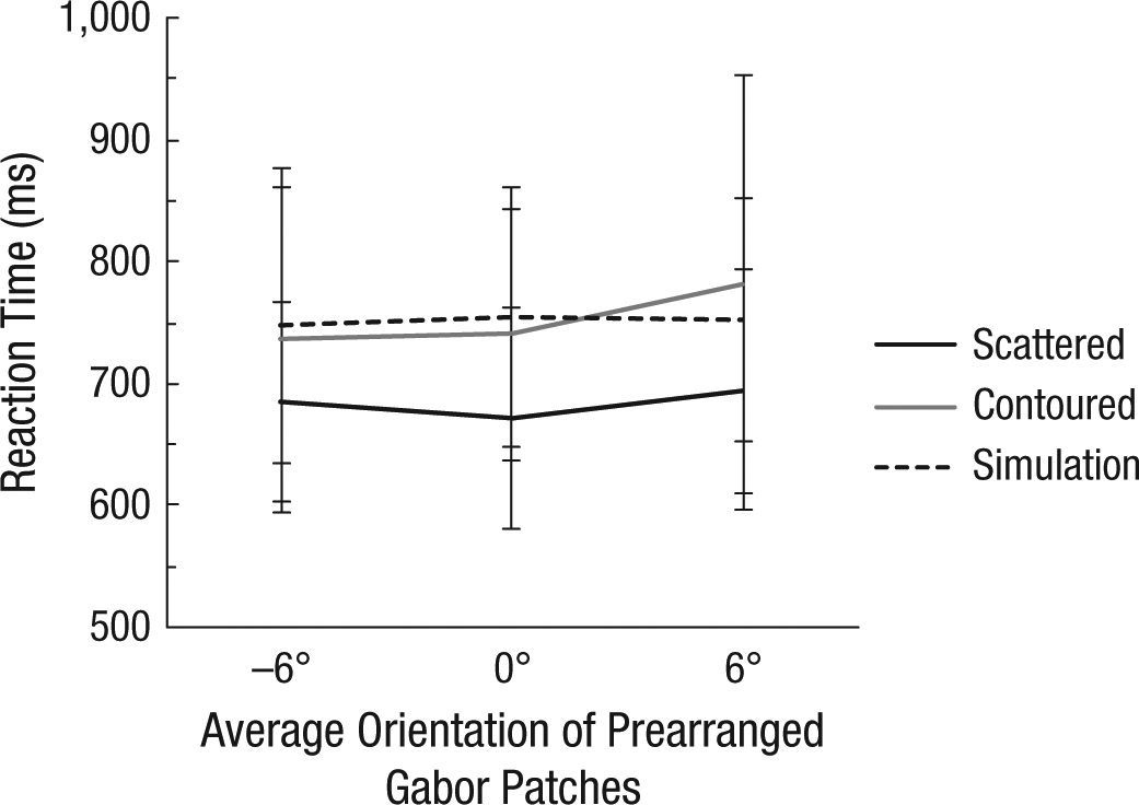
Mean reaction time predicted by the diffusion model, which accumulated perceptual evidence from 51 Gabor patches, excluding the 9 contour Gabor patches. Results are shown for each of the three average orientations of the prearranged Gabor patches, separately for the scattered and contoured conditions and for a simulation. The model was parametrized from the behavioral data in the scattered condition, and we predicted that the reaction times would be slower if the model ignored the contour Gabor patches. Error bars indicate 95% confidence intervals.

Second, the ideal observer simulation assumed that a participant would sample a few Gabor patches and calculated the average of the sampled patches. Figure 4a depicts the simulated responses of ideal observers that sampled one, two, or three out of the entire crowd of Gabor patches. The three-sample ideal observer almost approximated participants’ behavior in the scattered condition, F(6, 72) = 1.616, p = .155, η_p² = .119, but the one-sample ideal observer, F(6, 72) = 8.466, p < .001, η_p² = .414, and two-sample ideal observer, F(6, 72) = 2.993, p = .011, η_p² = .200, did not perform as well. Therefore, we used the three-sample ideal observer for further simulations. Without any constraints, the three-sample ideal observer failed to replicate the response biases in the contoured condition (Fig. 4b), as evidenced by a significant three-way interaction among type of data (behavior, simulation), contour orientation (counterclockwise, clockwise), and average orientation (seven levels), F(6, 72) = 2.778, p = .017, η_p² = .188. However, the ideal observer could predict behavioral responses nicely if it was constrained to not sample from the contour Gabor patches (Fig. 4c), as evidenced by a nonsignificant three-way interaction among type of data (behavior, simulation), contour orientation (counterclockwise, clockwise), and average orientation (seven levels), F(6, 72) = 0.375, p = .893, η_p² = .030. Both the diffusion model and the ideal observer simulation suggest that a parsimonious explanation to the response biases in the contoured condition is that entails ignoring orientation signals embedded in a contour.

Fig. 4.

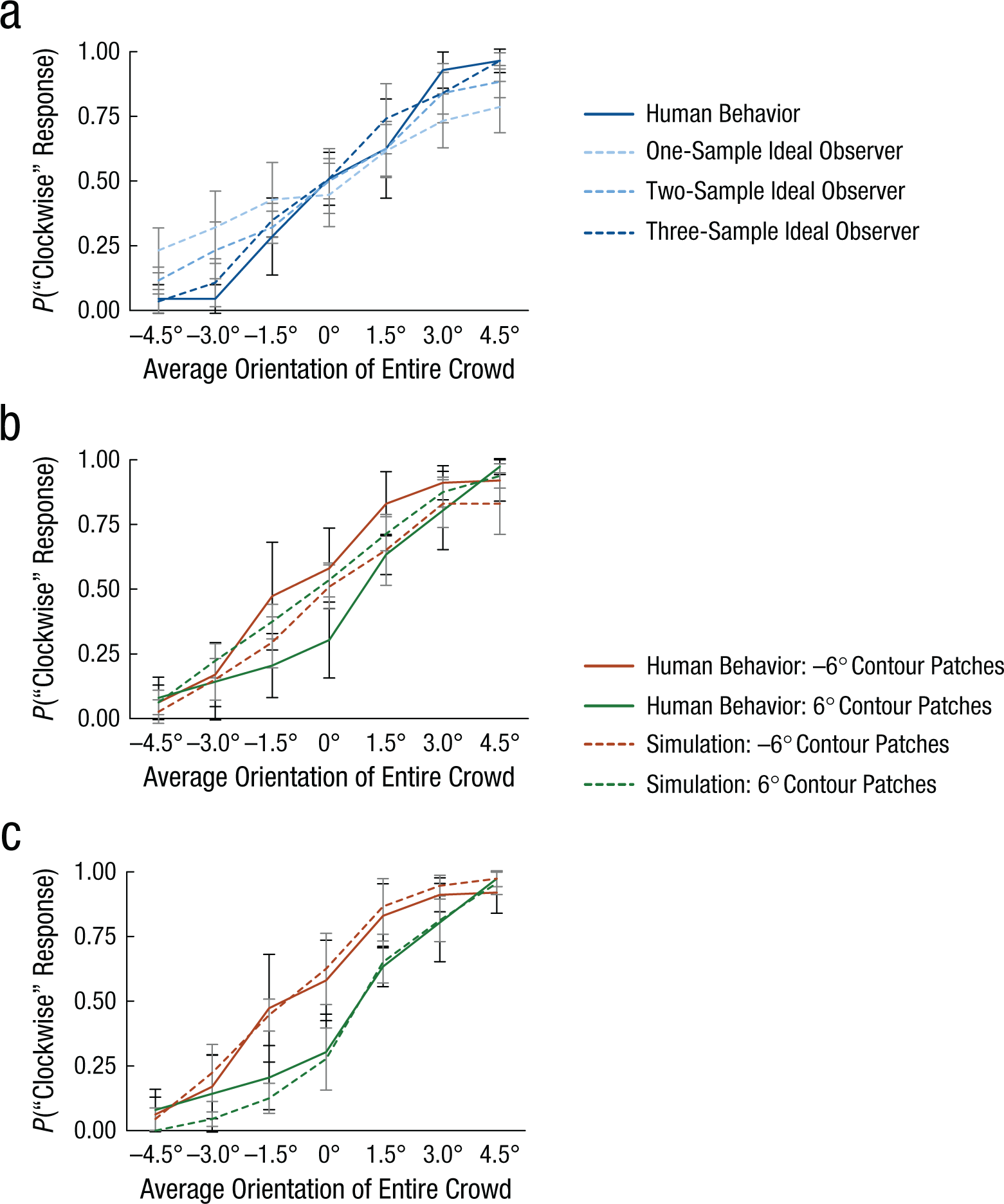
Simulated responses of the ideal observer plotted with the behavioral results. The probability of a “clockwise” response in the scattered condition (a) is shown for human participants and each ideal observer. The probability of a “clockwise” response in the contoured condition is shown for human participants and the three-sample observer when (b) the observer was able to sample from the entire crowd and (c) when it was constrained to avoid sampling from the contour Gabor patches. Responses in all graphs are shown for each average orientation of the entire crowd of Gabor patches. Error bars indicate 95% confidence intervals.

Discussion

The human visual system has the ability to estimate ensemble visual information, which may constitute building blocks of gist perception (Alvarez, 2011). The current study investigated whether spatial configuration of objects could provide boundary conditions for ensemble representation, thus enabling the visual system to form different ensembles for different perceptual groups having similar features. In the behavioral experiment, participants determined the average orientation of a crowd of Gabor patches when some of the patches formed a contour. Their responses were biased against the contour orientation, suggesting that the orientation signals embedded in the contour were ignored in the averaging. Two simulation approaches, analogous to different strategies participants might employ, predicted behavioral responses well only when the models ignored orientations of the contour Gabor patches.

The tendency to ignore a contour inside a surface can be beneficial in scene perception. If an object is surrounding another small object, it is likely that the small object is in front of and occluding part of the surrounding object. If the visual system is interested in the surrounding object, it is efficient to ignore visual features of the small object and assume that the occluded part of the surrounding object has the same ensemble as the visible part. A stained-glass window is a good example of exploiting this tendency. People see a picture of a character or an object despite the window frame splitting the character or object into several pieces. Adjacent pieces of glass with the same color are perceived as a uniform surface behind the window frame such that the colored surfaces constitute the whole picture.

It is not a new idea that grouping influences the formation of ensembles. Grouping of visual elements by color (Brady & Alvarez, 2011), location (Lew & Vul, 2015), Gestalt principles (Corbett, 2017), and synchrony (Elias, Dyer, & Sweeny, 2017) has been shown to bias participants’ reports on target items such that the target features assimilate to the average of a group. This assimilation suggests that the visual system represents visual elements as an ensemble, thereby reducing redundant information in the group of elements. It is reasonable to assume that the visual elements in the same group have several features in common. Thus the visual system can effectively represent large numbers of visual elements that would exceed capacity limits if processed individually. In previous studies, participants were asked to process numbers of objects exceeding the conventional capacity limit of three to four items (Luck & Vogel, 1997; Zhang & Luck, 2008). Participants might actively utilize ensembles to effectively perform the given tasks. As a result, it remains unclear whether the visual system would represent multiple ensembles for different groups even when it is unnecessary. In the current study, participants’ task was to integrate all visual features, regardless of their perceptual groups. If the visual system represents multiple ensembles, all groups (i.e., contour and surface) should be considered when determining the average orientation.

The current study is the first to reveal the inability to integrate features of different perceptual groups characterized by the spatial configuration. Previous studies have shown that the visual system can utilize ensembles to reduce redundant information. In exchange for this ability, individual visual elements lost precision on visual features: The features were biased toward ensemble information. Thus, individual visual features became less segregable from an ensemble. However, the inability to segregate a target feature from an ensemble is not the same as the ability to integrate that feature with others. We investigated this unclarified ability and found that the spatial configuration of features constrained their integration in such a way that the resulting ensemble representation ignored the individual contributions from the elements of different perceptual groups. Our results suggest that an ensemble is not a simple average of visual features. Rather, it is a bundle of visual elements that encloses features in the same perceptual group. This ensemble may be used to represent object properties in subsequent visual processing. An ensemble reflects effective properties of a surface, compensating for the occluded part.

In addition, simulation results of the current study have an important implication regarding ensemble representation’s incorporation of visual features of the entire objects versus a few that the visual system can handle at once (e.g., Allik, Toom, Raidvee, Averin, & Kreegipuu, 2013). As the task was to determine the average orientation of the entire array of Gabor patches, the best strategy for the ideal observer would be to sample from the entire array. The observer using that strategy (i.e., the three-sample ideal observer without constraints) accurately judged the average orientation, unlike human participants, who showed response biases against the contour orientation. If the visual system is going to sample a few Gabor patches, the best strategy may be to sample them regardless of their perceptual groups. This strategy ensures bias-free and fast decision making. The second-best strategy may be to consider perceptual groups and sample with different probabilities on the basis of the size of perceptual groups (e.g., sample one Gabor patch from the contour and two Gabor patches from the rest). In any case, ignoring Gabor patches in a specific perceptual group (e.g., a contour) will not be a good strategy. The more parsimonious explanation would be that the visual system represents different ensembles depending on the spatial configuration of elements comprising that scene.

In conclusion, we hypothesized that the ensemble representation would reflect the spatial configuration of objects. The visual system should build different ensembles for different groups of visual elements or it could not deal with a complex visual scene crowded with similar objects. As expected, participants could not integrate the visual feature of a contour to that of the surrounding surface, although they were asked to report the average visual feature of all the stimuli. Our results, in other words, highlight this constraint: The visual system cannot integrate visual features of different perceptual groups. This constraint may provide an efficient way to represent an occluded object in a real-world visual scene.

Footnotes

Acknowledgements

We thank Randolph Blake for his helpful comments.

Action Editor

Edward S. Awh served as action editor for this article.

Author Contributions

O. Cha and S. C. Chong jointly developed the study concept and design. Testing and data collection were performed by O. Cha. Both authors analyzed and interpreted the data. O. Cha drafted the manuscript, and S. C. Chong provided critical revisions. Both authors approved the final version of the manuscript for submission.

Declaration of Conflicting Interests

The author(s) declared that there were no conflicts of interest with respect to the authorship or the publication of this article.

Funding

This work was supported by a grant from the National Research Foundation of Korea, which is funded by the Korean government (NRF-2016R1A2B4016171).

Open Practices

All data and materials have been made publicly available via the Open Science Framework and can be accessed at https://osf.io/b9tse/. The complete Open Practices Disclosure for this article can be found at https://journals-sagepub-com.web.bisu.edu.cn/doi/suppl/10.1177/0956797617735533. This article has received badges for Open Data and Open Materials. More information about the Open Practices badges can be found at .

References

Allik

Toom

Raidvee

Averin

Kreegipuu

(2013). An almost general theory of mean size perception. Vision Research, 83, 25–39. doi:10.1016/j.visres.2013.02.018

Alvarez

G. A.

(2011). Representing multiple objects as an ensemble enhances visual cognition. Trends in Cognitive Sciences, 15, 122–131. doi:10.1016/j.tics.2011.01.003

Alvarez

G. A.

Oliva

(2008). The representation of simple ensemble visual features outside the focus of attention. Psychological Science, 19, 392–398. doi:10.1111/j.1467-9280.2008.02098.x

Ariely

(2001). Seeing sets: Representation by statistical properties. Psychological Science, 12, 157–162. doi:10.1111/1467-9280.00327

Bauer

(2009). The danger of trial-by-trial knowledge of results in perceptual averaging studies. Attention, Perception, & Psychophysics, 71, 655–665. doi:10.3758/APP.71.3.655

Brady

T. F.

Alvarez

G. A.

(2011). Hierarchical encoding in visual working memory: Ensemble statistics bias memory for individual items. Psychological Science, 22, 384–392. doi:10.1177/0956797610397956

Brainard

(1997). The Psychophysics Toolbox. Spatial Vision, 10, 433–436. doi:10.1163/156856897X00357

Burr

Ross

(2008). A visual sense of number. Current Biology, 18, 425–428. doi:10.1016/j.cub.2008.02.052

Carrasco

Ling

Read

(2004). Attention alters appearance. Nature Neuroscience, 7, 308–313. doi:10.1038/nn1194

10.

Chong

S. C.

Treisman

(2003). Representation of statistical properties. Vision Research, 43, 393–404. doi:10.1016/S0042-6989(02)00596-5

11.

Chong

S. C.

Treisman

(2005). Attentional spread in the statistical processing of visual displays. Perception & Psychophysics, 67, 1–13. doi:10.3758/BF03195009

12.

Corbett

J. E.

(2017). The whole warps the sum of its parts: Gestalt-defined-group mean size biases memory for individual objects. Psychological Science, 28, 12–22. doi:10.1177/0956797616671524

13.

Dakin

S. C.

Watt

R. J.

(1997). The computation of orientation statistics from visual texture. Vision Research, 37, 3181–3192. doi:10.1016/S0042-6989(97)00133-8

14.

Elias

Dyer

Sweeny

T. D.

(2017). Ensemble perception of dynamic emotional groups. Psychological Science, 28, 193–203. doi:10.1177/0956797616678188

15.

Field

D. J.

Hayes

Hess

R. F.

(1993). Contour integration by the human visual system: Evidence for a local “association field.” Vision Research, 33, 173–193. doi:10.1016/0042-6989(93)90156-Q

16.

Fründ

Haenel

N. V.

Wichmann

F. A.

(2011). Inference for psychometric functions in the presence of nonstationary behavior. Journal of Vision, 11(6), Article 16. doi:10.1167/11.6.16

17.

Kleiner

Brainard

Pelli

(2007, August). What’s new in Psychtoolbox-3? Tutorial session presented at the 30th European Conference on Visual Perception, Arezzo, Italy.

18.

Larson

A. M.

Freeman

T. E.

Ringer

R. V.

Loschky

L. C.

(2014). The spatiotemporal dynamics of scene gist recognition. Journal of Experimental Psychology: Human Perception and Performance, 40, 471–487. doi:10.1037/a0034986

19.

Larson

A. M.

Loschky

L. C.

(2009). The contributions of central versus peripheral vision to scene gist recognition. Journal of Vision, 9(10), Article 6. doi:10.1167/9.10.6

20.

Lee

Baek

Chong

S. C.

(2016). Perceived magnitude of visual displays: Area, numerosity, and mean size. Journal of Vision, 16(3), Article 12. doi:10.1167/16.3.12

21.

Lew

T. F.

Vul

(2015). Ensemble clustering in visual working memory biases location memories and reduces the Weber noise of relative positions. Journal of Vision, 15(4), Article 10. doi:10.1167/15.4.10

22.

Gilbert

C. D.

(2002). Global contour saliency and local colinear interactions. Journal of Neurophysiology, 88, 2846–2856. doi:10.1152/jn.00289.2002

23.

Ling

Carrasco

(2006). Sustained and transient covert attention enhance the signal via different contrast response functions. Vision Research, 46, 1210–1220. doi:10.1016/j.visres.2005.05.008

24.

Livne

Sagi

(2007). Configuration influence on crowding. Journal of Vision, 7(2), Article 4. doi:10.1167/7.2.4

25.

Luck

S. J.

Vogel

E. K.

(1997). The capacity of visual working memory for features and conjunctions. Nature, 390, 279–281. doi:10.1038/36846

26.

Mareschal

Morgan

M. J.

Solomon

J. A.

(2010). Attentional modulation of crowding. Vision Research, 50, 805–809. doi:10.1016/j.visres.2010.01.022

27.

Morgan

Dillenburger

Raphael

Solomon

J. A.

(2012). Observers can voluntarily shift their psychometric functions without losing sensitivity. Attention, Perception, & Psychophysics, 74, 185–193. doi:10.3758/s13414-011-0222-7

28.

Myung

I. J.

(2003). Tutorial on maximum likelihood estimation. Journal of Mathematical Psychology, 47, 90–100. doi:10.1016/S0022-2496(02)00028-7

29.

Parkes

Lund

Angelucci

Solomon

J. A.

Morgan

(2001). Compulsory averaging of crowded orientation signals in human vision. Nature Neuroscience, 4, 739–744. doi:10.1038/89532

30.

Pelli

(1997). The VideoToolbox software for visual psychophysics: Transforming numbers into movies. Spatial Vision, 10, 437–442. doi:10.1163/156856897X00366

31.

Polat

Sagi

(1994). The architecture of perceptual spatial interactions. Vision Research, 34, 73–78. doi:10.1016/0042-6989(94)90258-5

32.

Ratcliff

Rouder

J. N.

(1998). Modeling response times for two-choice decisions. Psychological Science, 9, 347–356. doi:10.1111/1467-9280.00067

33.

Utochkin

I. S.

(2015). Ensemble summary statistics as a basis for rapid visual categorization. Journal of Vision, 15(4), Article 8. doi:10.1167/15.4.8

34.

Wolfe

J. M.

Võ

M. L. H.

Evans

K. K.

Greene

M. R.

(2011). Visual search in scenes involves selective and nonselective pathways. Trends in Cognitive Sciences, 15, 77–84. doi:10.1016/j.tics.2010.12.001

35.

Zhang

Luck

S. J.

(2008). Discrete fixed-resolution representations in visual working memory. Nature, 453, 233–235. doi:10.1038/nature06860

Supplementary Material

Please find the following supplemental material available below.

For Open Access articles published under a Creative Commons License, all supplemental material carries the same license as the article it is associated with.

For non-Open Access articles published, all supplemental material carries a non-exclusive license, and permission requests for re-use of supplemental material or any part of supplemental material shall be sent directly to the copyright owner as specified in the copyright notice associated with the article.

0.00 MB

0.58 MB