Computational fluid dynamics investigation into flow behavior and acoustic mechanisms at the trailing edge of an airfoil

Abstract

Airfoil self-noise or trailing edge noise and shear noise were investigated computationally for a NACA 0012 airfoil section, focusing on noise mechanisms at the trailing edge to identify and understand sources of noise production using ANSYS Fluent. A two-dimensional computational fluid dynamics simulation has been performed for 0°, 8°, and 16° airfoil angles of attack capturing surface pressure contours, contours of turbulent intensity, contours of surface acoustic power level, vorticity magnitude levels across the airfoil profile, and x- and y-directional self-noise and shear noise sources across the airfoil profile. The results indicate that pressure gradients at the upper surface do increase as the angle of attack increases, which is a measure of vortices near the surface of the trailing edge associated with turbulence cease as the boundary layer begins to separate. Comparison of the turbulent intensity contours with surface acoustic power level contours demonstrated direct correlation between the energy contributed by turbulent structures (i.e. vortices) and the level of noise measured at the surface and within the boundary layer of the airfoil. As angle of attack is increased, both x and y sources have the same trends; however, y sources (perpendicular to the free-stream flow) appear to have a bigger impact as angle of attack is increased. Furthermore, as the angle of attack increased, shear noise contributes less and less energy further downstream of the airfoil and becomes dominated by noise energy from vortical structures within turbulence. The two-dimensional computational fluid dynamics simulation revealed that pressure, turbulent intensity, and surface acoustic power contours further corroborated the previously tested noise observations phenomena at the trailing edge of the airfoil.

Keywords

Airfoil self-generated noise trailing edge noise turbulent intensity surface acoustic power level shear noise

Introduction

Stringent regulations on noise radiated by aircraft engines are getting tighter, and this is due to forecast of future explosive growth in air transport that requires special attention in reducing noise emissions, especially during landing approaches in airport-neighboring communities. Therefore, knowledge of noise sources and mechanisms of noise production at the trailing edge of an airfoil is getting high priority in order to address and mitigate aircraft noise emissions. Furthermore, addressing the noise productions has wider implications on design of wind turbine blades, turbomachinery, ship hulls, and airfoil design.

A review of self-generated noise mechanisms associated with subsonic flow surrounding an airfoil was defined by Brooks et al.¹ Five airfoil self-generated noise mechanisms producing noise were described. At high Reynolds numbers, turbulent boundary layer is developed over most of the airfoil, and broadband noise is generated as turbulence passes the trailing edge. At low Reynolds numbers, laminar boundary develops at most of the airfoil, due to laminar boundary layer instabilities which cause vortex shedding and noise associated with the trailing edge. At non-zero angle of attack, flow separation at the trailing edge on the upper surface and noise are generated due to turbulence shed vorticities. At higher angle of attack, large separation of the flow is encountered and the airfoil experiences deep stall; in this regime, low-frequency noise is generated. Another source of radiated noise is vortex shedding in the wake of blunt trailing edge. The remaining noise sources are radiated due to development of airfoil tip vortices from turbulent flow. It is worth noting that boundary layer separation will generate several tonal peaks that are superimposed on the broadband noise, and these are perhaps due to vortex shedding associated with the airfoil trailing edge.

An airfoil self-noise or trailing edge noise (TE) is defined when noise is generated due to vortical disturbances which are transformed into acoustical ones once they are convected downstream of the trailing edge. Roger and Moreau² had noted that attached or separated turbulent boundary layer at the trailing edge generates broadband noise; however, whistles are generated due to laminar boundary disturbances. The self-noise production was addressed by Roger and Moreau³ as a balance of forces encountered during the development of vortices traveled downstream due to pressure gradients and induced centrifugal forces. The geometrical singularity at the trailing edge causes further amplification of the radiated noise downstream as the flow maintains its adjustment through rapid reorganization of the vortical structures.

Two streams of ideas gained wide acceptance from the scientific noise communities, in relation to analytical analysis of self-noise generation. The first developed by Ffowcs Williams and Hall,⁴ where the noise radiated by the vortical disturbances of the boundary layer downstream of the trailing edge is related to the vortical velocity at the trailing edge. Amiet⁵ and Howe⁶ introduced the second approach which relates the far-field acoustic signature statistics to the aerodynamic wall pressure statistics at some point upstream of the trailing edge. Based on this methodology, the surface pressure is utilized as an equivalent acoustic source, though sound is generated due to the velocity field. An experimental verification for the second approach was accomplished by Brooks et al.¹ and Roger and Moreau³ and was carried out successfully by Brooks and Hodgson.⁷

Experimental data

The experimental apparatus of the NACA 0012 airfoil including the embedded microphone locations as a function of the chord length and analysis of the acoustic data were described and reported by Jackson and Dakka.⁸ To summarize the experimental findings for the energy/frequency spectra, toward the trailing edge, the overall noise seen to be reduced and a reduction of the pressure can be observed. It appears that at the trailing edge, for smaller frequencies, the energy is relatively lower initially (than toward the leading edge), whereas past a certain point, noise energy toward the trailing edge is lost at a faster rate than at the leading edge. In general, for a laminar boundary layer, they also appear to decrease in magnitude with angle of attack, whereas under a turbulent boundary layer, the Strouhal numbers reported increase in magnitude with angle of attack.

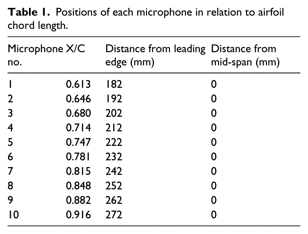
It is interesting to note that the first four peak frequencies reported by Jackson and Dakka⁸ do not deviate significantly between measurements at each angle of attack increase. The first, fifth, and “knee” frequencies are not related harmonically and must be related to the behavior of the flow itself or due to shear interactions between the flow and the airfoil surface. Based on frequency spectra in the range of around 1–10 kHz, the steepening of the slope with increase in angle of attack was observed at microphone 1 and also the decay of the slopes of microphones 5 and 10 (see Table 1 for chord locations). These observations could also be related to the steepening and magnitude of the adverse pressure gradient and would suggest that for a given point, for different angles of attack, vortices are at different stages of development.

Table 1.

Positions of each microphone in relation to airfoil chord length.

Microphone no.	X/C	Distance from leading edge (mm)
1	0.613	182
2	0.646	192
3	0.680	202
4	0.714	212
5	0.747	222
6	0.781	232
7	0.815	242
8	0.848	252
9	0.882	262
10	0.916	272

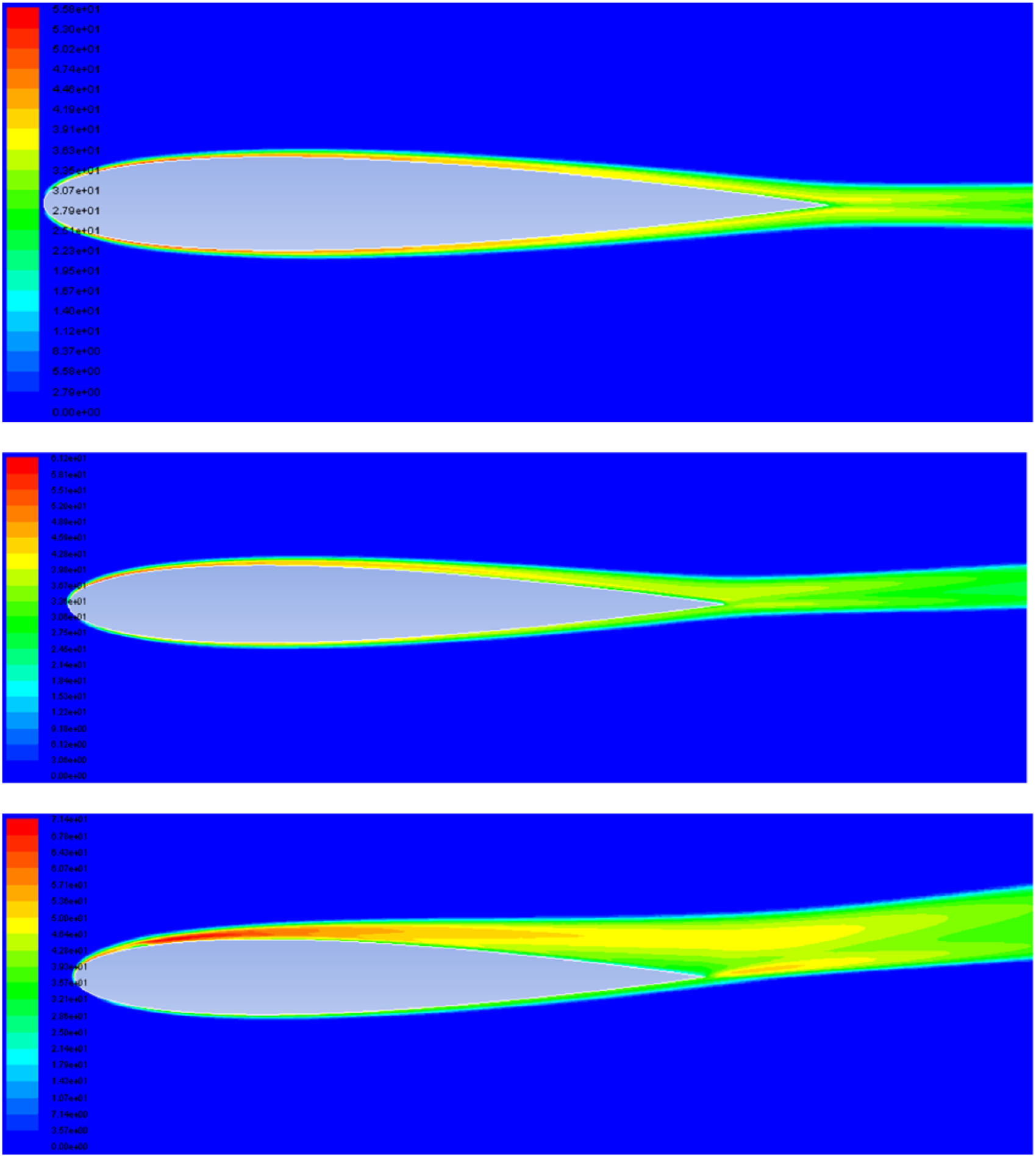
Another interesting observation based on the measured data is the fact that the sound pressure level stark behavior within the 3–10 kHz region and the 1–3 kHz region. The sound pressure level at microphone 10 appears to decay sooner as compared with microphone 5 as the angle of attack increases but still significantly higher than microphone 1, while for 1–3 kHz, sound pressure level for microphone 10 is higher than microphone 5. This would suggest that there is in fact a higher amount of turbulent energy at microphone 5 in the region of about 3–10 kHz, than there is at microphone 10, for lower angles of attack. Between 1 and 3 kHz, it was suggested that the frequency spectra show a measure of the far-field noise energy; microphone 1 measures less energy in this portion because the boundary layer is still relatively small, effectively it may be measuring the free-stream flow energy outside of the boundary layer, whereas microphones 5 and 10 are actually measuring energy within the boundary layer, which has grown to a sufficient size at this point, where microphone 5 detects the turbulent energy slightly closer to the outer edge of the boundary layer than does microphone 10, which measures a higher turbulent energy. Looking at the contours of turbulent intensity from the computational fluid dynamics (CFD) simulation in Figure 7, this visualization becomes clearer and explains why microphone 10 measures higher energy than microphone 5, as angle of attack is increased, in the 1–3 kHz band.

However, between 3 and 10 kHz, a phenomenon which would explain the differences in slope at microphones 5 and 10 is separation stall noise; as angle of attack is increased, the boundary layer at microphone 10 has a much higher affinity to separate (higher local Reynolds number) than microphone 5 (and microphone 1); therefore, within the near-field region, there is less energy due to small-scale vortical formations than there is at microphone 5, and effectively, the only noise energy being measured is due to the back-draft of wake flow, which would also explain why the slope of microphone 10 becomes closer to microphone 5 as angle of attack is increased, since microphone 5 is also beginning to detect noise mechanisms due to wake flow. This theory was further supported⁸ by the calculations of boundary layer thickness, skin friction, and wall shear stress, which show that viscous forces do in fact reduce with location along the trailing edge.

CFD analysis

A two-dimensional (2D) CFD simulation has been performed for 0°, 8°, and 16° angles of attack. The methodology and results are presented consequently.

Methodology

Initially, a mesh, Figures 1 and 2, was generated for the NACA 0012 geometry with conditions similar to those tested in the physical acoustic wind tunnel testing.⁸ This 2D mesh domain involved an enclosure of around 5 m × 4 m, with a domed inlet. Sufficient space was left between the inlet and NACA 0012 airfoil (of chord 0.297 m), and also between the trailing edge and the fluid outlet, in order to accurately capture free-stream flow, that is, no intrinsic pressure sources could affect the external flow and thus the flow around the airfoil was accurately captured. The domed inlet allowed the inlet velocity components to be changed, thus allowing the same effect of rotating the airfoil and hence its angle of attack could be changed. Three simulations were performed for 0°, 8°, and 16°.

Figure 1.

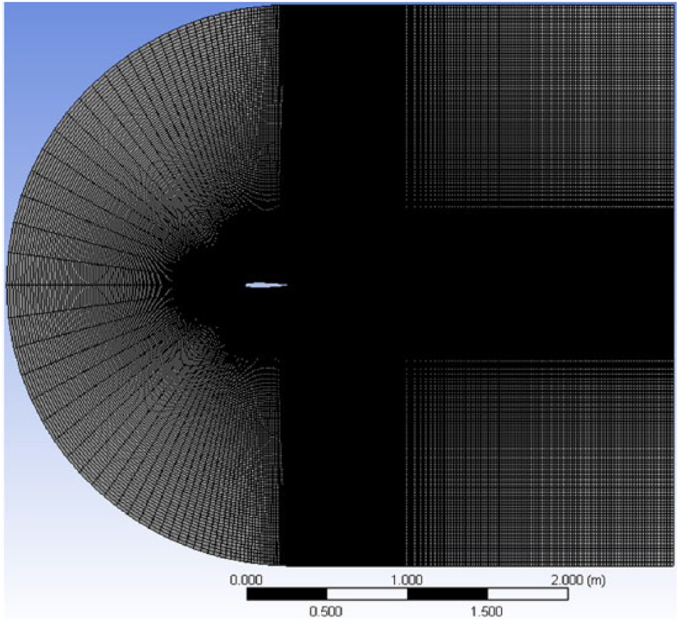
Generated mesh for 2D CFD simulation.

Figure 2.

Close-up of airfoil and mesh.

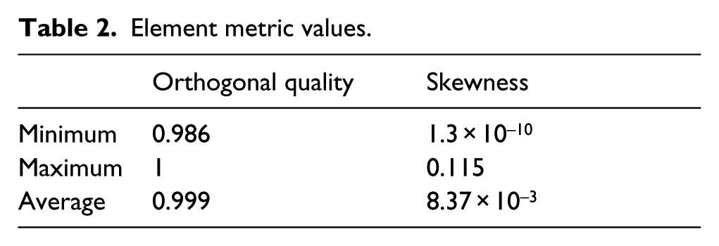
The generated mesh was of a very high quality, necessary for representative propagation of flow (essentially numerical calculations) between mesh cells (elements). There were 220,472 elements, the smallest of which being at the surface and in high activity regions around the airfoil (such as the boundary layer and wake). Figure 3 shows the element metric graphs of orthogonal quality (a measure of quality for the incident quadrilateral cell mesh) and skewness (a measure of how stretched a mesh cell is).The graphs show how the majority of mesh elements are of extremely high quality and are minimally skewed. Table 2 gives values for the minimum, maximum, and average of these element metrics (values range from 0 to 1). The airfoil surface was given the characteristics of the same material used for the physical model, acrylonitrile butadiene styrene (ABS), and boundary conditions represented the characteristics of air at room temperature and with the same parameters as at sea level, the same environment in which the physical acoustic testing was done. The numerical solution method used was the two-equation, transient-based shear stress transport (SST) k-ω model, with a broadband noise, acoustics model solver. Other than solving for conservation of mass, momentum, and energy, the parameters “k” and “ω” are the main functions calculated in this solver method, k being turbulent kinetic energy and ω being the specific dissipation rate of the turbulence.⁹ The “Shear Stress Transport” (SST) is an added factor in the model, developed by Menter et al.,¹⁰ which increases accuracy for near wall treatment of the flow by considering effects of shear stress. The model is widely used for predicting aerodynamic flows with strong adverse pressure gradients and boundary layer separation,¹⁰ and thus is sufficient for the current simulation.

Figure 3.

Mesh cell orthogonal quality (left) and mesh cell skewness (right).

Table 2.

Element metric values.

	Orthogonal quality	Skewness
Minimum	0.986	1.3 × 10–10
Maximum	1	0.115
Average	0.999	8.37 × 10–3

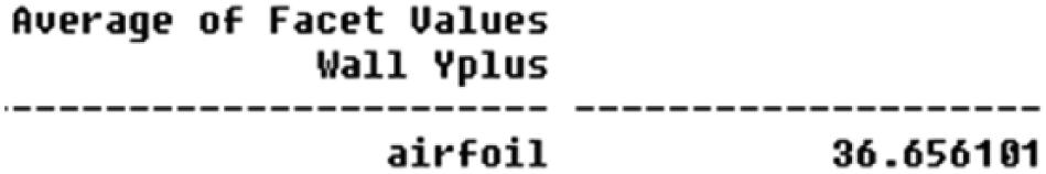
In order for the solver to accurately predict the velocity of flow near to the airfoil surface, a value known as y+ has to be within a certain value. This parameter is a non-dimensional wall distance which is defined as follows: $y^{•} \equiv u_{*} y / v$ , where the nominator is the multiplication of the friction velocity, $u_{*}$ and distance to nearest wall, y; the denominator is the local kinematic viscosity of the fluid. For an accurate prediction for the k-ω model, it was stated that even for y+ values between 2 and 100, the shear stress at the wall computed varies at less than 2%.¹⁰ Figure 4 gives the reported average y+ value across the airfoil surface for the current simulation. The residual convergence graph (Figure 5) shows how the iterative numerical calculations of the solver were reduced to within an extremely low error bar for each parameter (x-velocity, y-velocity, k, ω, and continuity).

Figure 4.

Reported average y+ value for NACA 0012 2D CFD simulation.

Figure 5.

Solver residuals convergence graph against iterations.

It can be seen from Figure 5 that a highly accurate error bar of at least 1e−06 was achieved, meaning that calculated values are correct to within this limit (x and y velocities converged at around 1e−08; k and ω residuals converged in the region of 1e−12). Note how there are three sections to the graph; each represents a solver “order”; initial simulation was done at first order, then second, then finally, a third-order solution was produced, to increase the precision of results.

Data and results

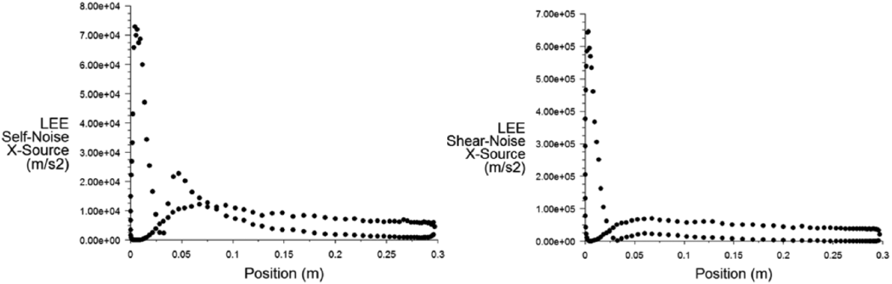
Several results have been obtained relating to noise mechanisms across the NACA 0012 airfoil at 20 m/s; these are pressure coefficient, turbulent intensity (%), surface acoustic power level (dB), self-noise, and shear noise from x-directional sources; and self-noise and shear noise from y-directional sources (units are m/s²), this is illustrated in Figures 6 –9.

Figure 6.

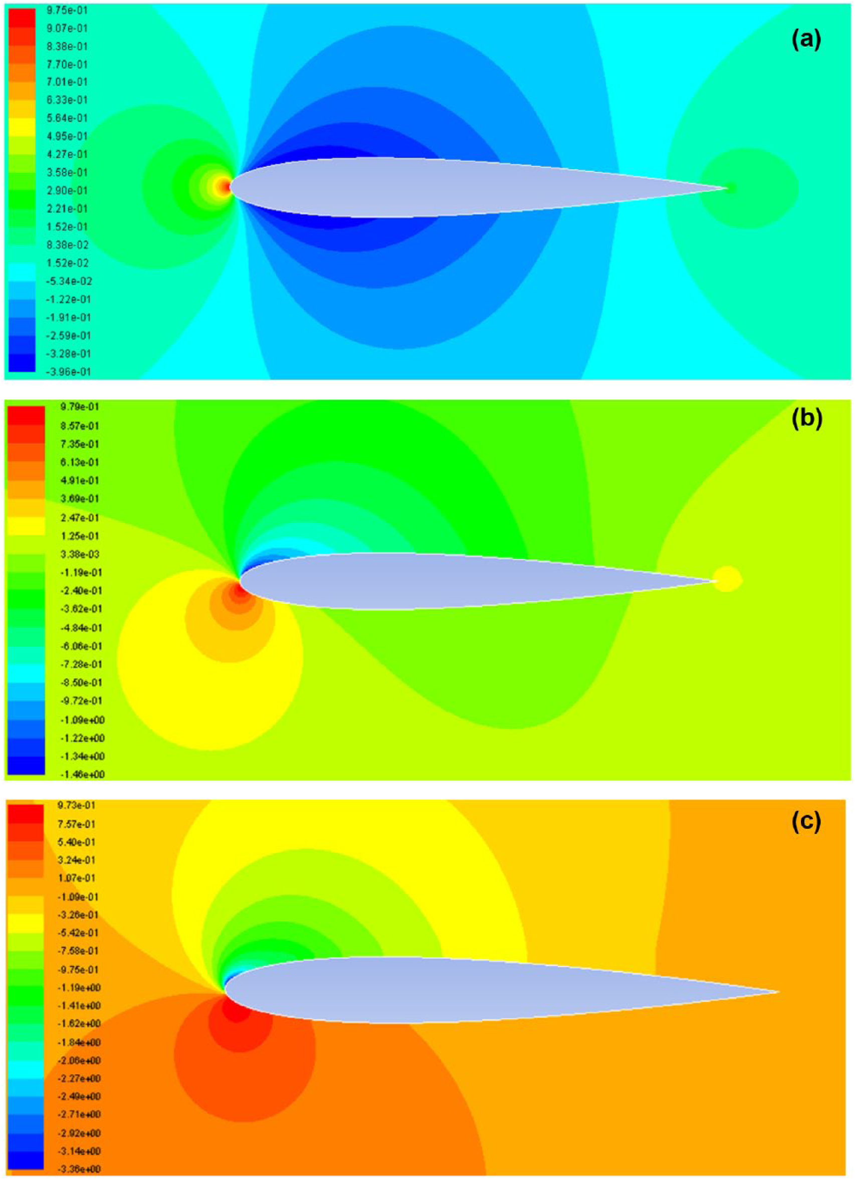
Contours of pressure coefficient for (a) 0°, (b) 8°, and (c) 16° angle of attack.

Figure 7.

Contours of turbulent intensity for (a) 0°, (b) 8°, and (c) 16° angle of attack.

Figure 8.

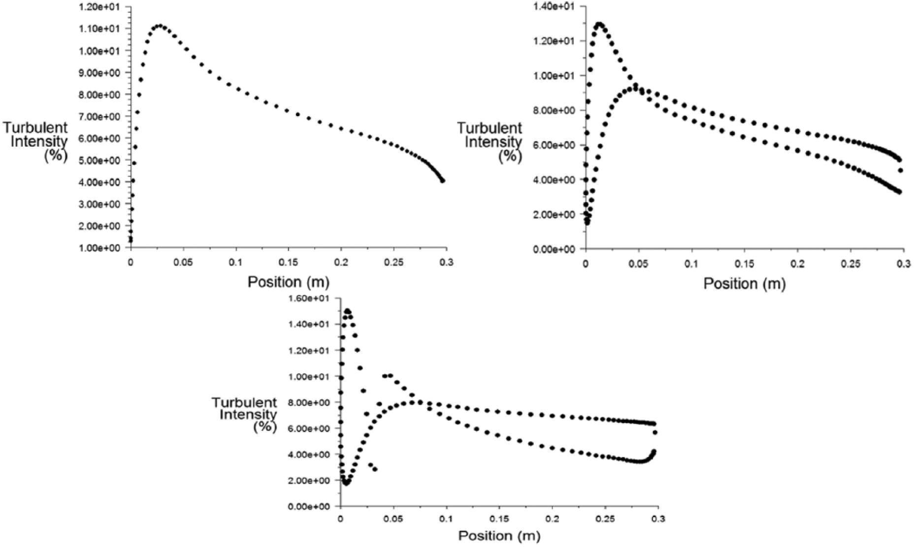
Graphs of turbulent intensity across the airfoil profile for 0° (top-left), 8° (top-right), and 16° (bottom).

Figure 9.

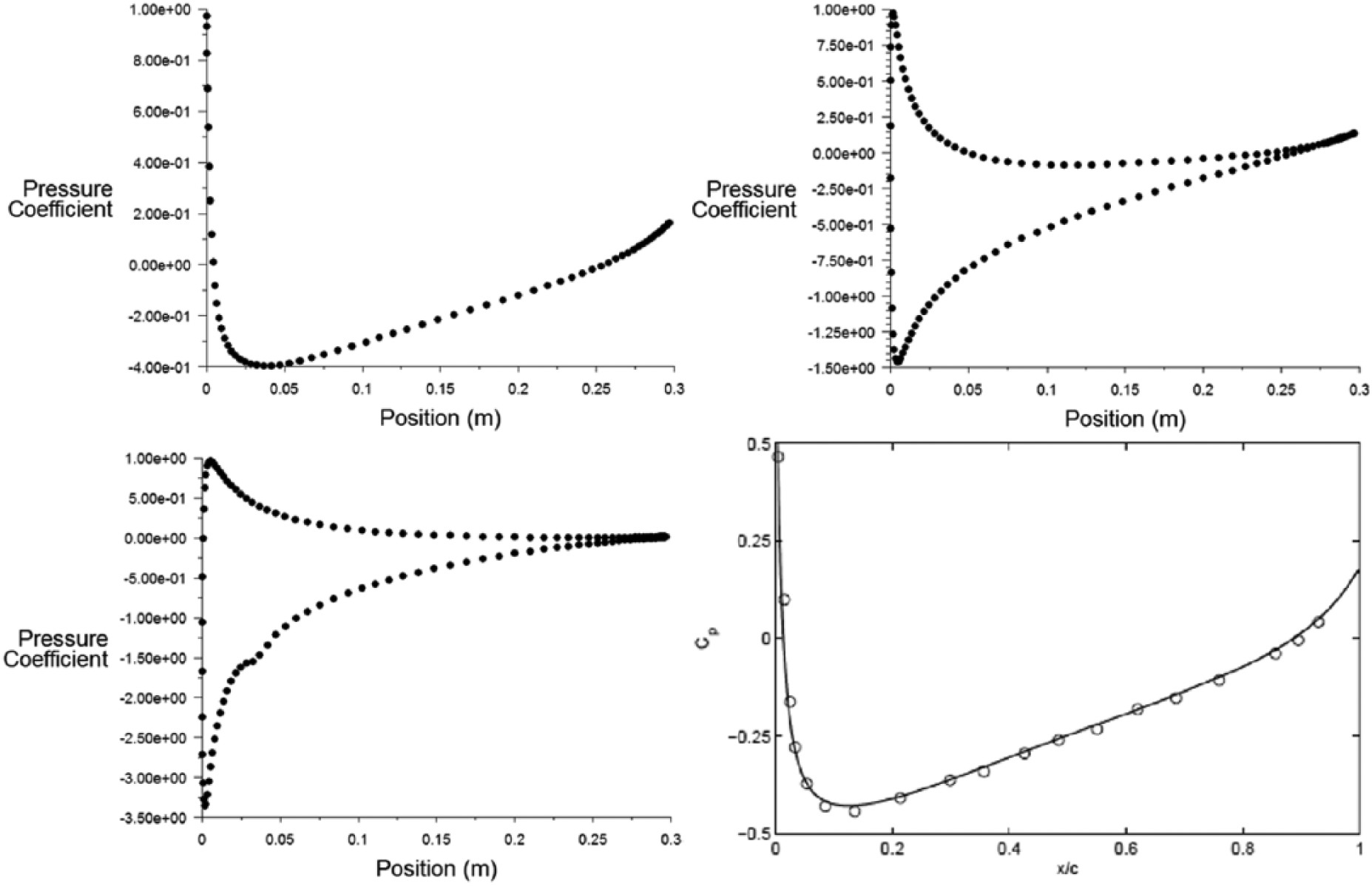
Graphs of pressure coefficient across the airfoil profile for 0° (top-left), 8° (top-right), and 16° (bottom-left). A validation source is also included for comparison with 0° (bottom-right) (Marsden et al.¹¹).

Note that an individual validation section is unnecessary for this CFD simulation, since the method of ensuring a quality mesh and simulation environment has been described in the previous section. However, the similarity between the coefficient of pressure graphs for 0° in the present simulation and against the three-dimensional (3D) simulation of a much similar NACA 0012 airfoil (and Reynolds number) at 0° by Marsden et al.¹¹ is clear—values are very similar to insignificant deviation, proving that the simulation which has been performed has achieved valid results. Results compiled will henceforth be discussed.

CFD simulation

The inclusion of CFD further supports the claims made in the previous section on the summary of the experimental data. When the simulated pressure distributions (represented by contours in Figure 6 and graphs in Figure 9) are observed, it can be surmised that the adverse pressure gradients do in fact steepen, as expected, with angle of attack, and in Figure 9, the upper surface is represented by the bottom curve and the lower surface by the top curve (upper surface is negative, lower surface is positive).

When reviewing the turbulence intensity contours and graphs (Figures 8 and 9) against the contours and graphs of surface acoustic power level (Figures 10 and 11), it is clear that there is an almost direct correlation between the energy contributed by turbulent structures (i.e. vortices) and the level of noise measured at the surface and within the boundary layer of the airfoil. In the case of each of these graphs, the upper surface is represented by the curve which has a high peak at the location of the leading edge, which, as angle of attack is increased, trails off toward the trailing edge until some point at which the turbulence intensity (and hence surface acoustic power level) of the lower surface is higher. As suggested in the previous discussion on the physical acoustic testing, as the adverse pressure gradient along the upper surface boundary layer becomes stronger with angle of attack, vortices near to the surface of the trailing edge associated with turbulence cease as the boundary layer begins to separate, and this is reflected in the plots of vorticity (Figure 12) for each angle of attack. Of course, since the adverse pressure gradient of the lower surface straightens out with angle of attack, the boundary layer remains attached, and vorticity becomes stronger due to downstream turbulence.

Figure 10.

Contours of surface acoustic power level (dB) for (a) 0°, (b) 8°, and (c) 16° angle of attack.

Figure 11.

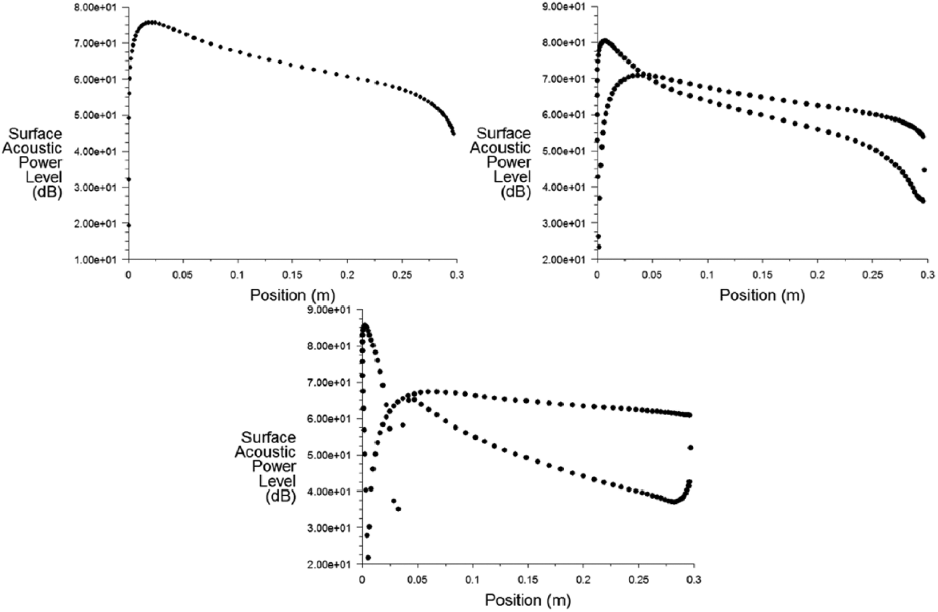
Graphs of surface acoustic power level (dB) across the airfoil profile for 0° (top-left), 8° (top-right), and 16° (bottom).

Figure 12.

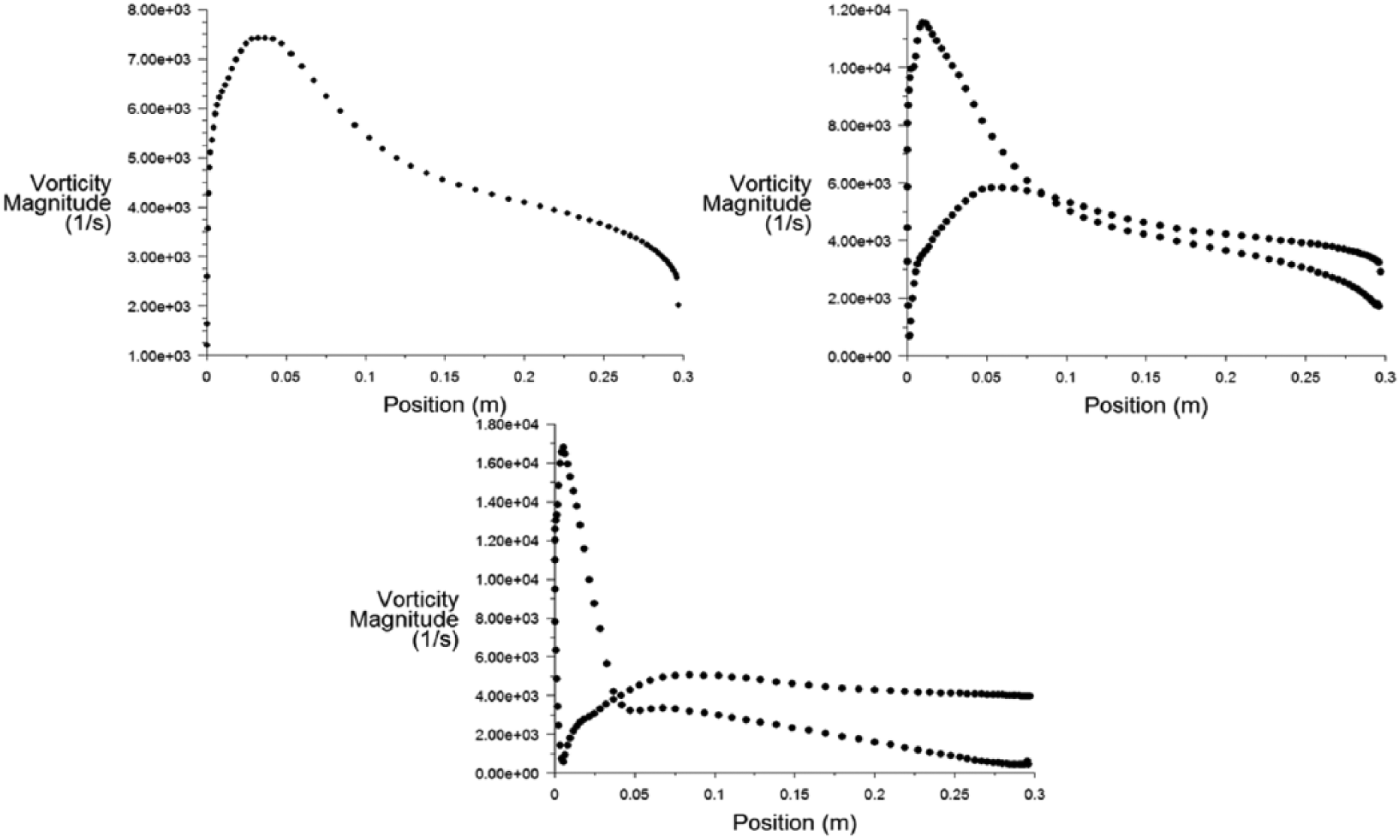
Graphs of vorticity magnitude (1/s) across the airfoil profile for 0° (top-left), 8° (top-right), and 16° (bottom).

Also, looking at the upper surface chord location × point of around 0.03 m for both the turbulence intensity and surface acoustic power level graphs at 16° angle of attack, a distinct trough can be seen, which, when looking closely at this point on the contour plots of Figures 7(c) and 10(c), can be seen to be due to a small-scale separation bubble, which then reattaches again to become part of the turbulent boundary layer.

A final discernment can be gained by viewing the x- and y-directional self-noise and shear noise source plots of Figures 13 –18; generally, as angle of attack is increased, both x and y sources have the same trends, yet, y sources (perpendicular to the free-stream flow) appear to have a bigger impact as angle of attack is increased. This solidifies the assumption made in the previous reported study⁸ and can be explained by the propagation of Tollmien–Schlichting waves, which of course increase in amplitude (a y-directional source) along the airfoil. Also, as the angle of attack is increased, x sources (viscous and shear effects) appear to have less of an effect with increase in angle of attack. These observations clearly show that as angle of attack is increased, shear noise contributes less and less energy further downstream of the airfoil and becomes dominated by noise energy from vortical structures within turbulence, such as Kelvin–Helmholtz instabilities.

Figure 13.

Graphs of x-directional noise sources (m/s²) across the airfoil profile for 0°, self-noise (left), and shear noise (right).

Figure 14.

Graphs of x-directional noise sources (m/s²) across the airfoil profile for 8°, self-noise (left), and shear noise (right).

Figure 15.

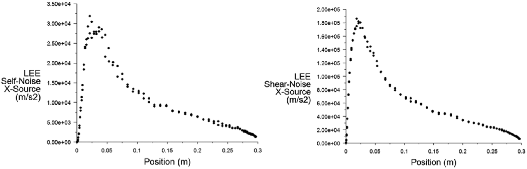
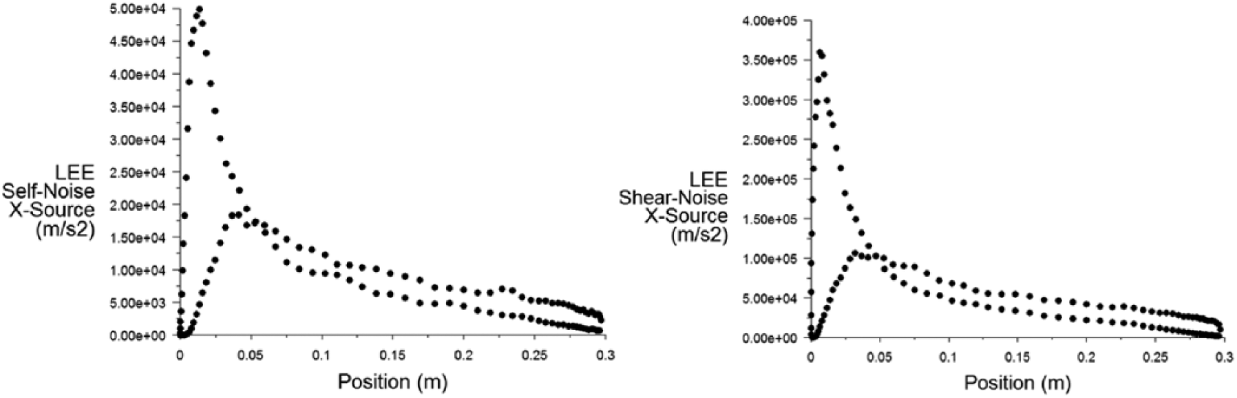
Graphs of x-directional noise sources (m/s²) across the airfoil profile for 16°, self-noise (left), and shear noise (right).

Figure 16.

Graphs of y-directional noise sources (m/s²) across the airfoil profile for 0°, self-noise (left), and shear noise (right).

Figure 17.

Graphs of y-directional noise sources (m/s²) across the airfoil profile for 8°, self-noise (left), and shear noise (right).

Figure 18.

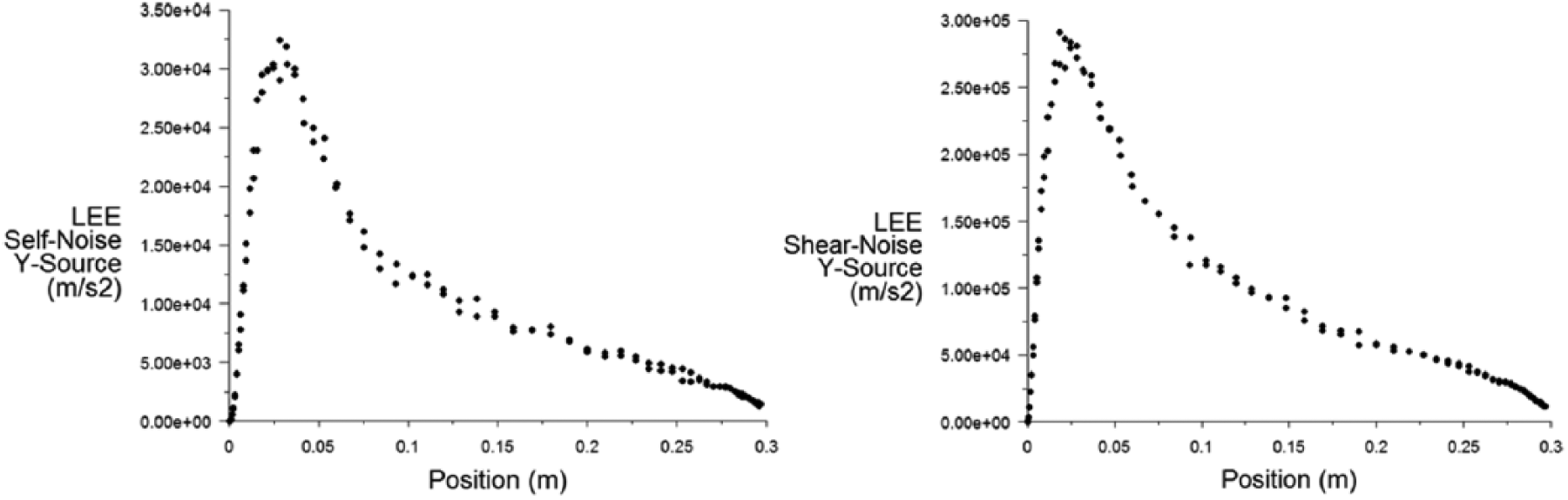
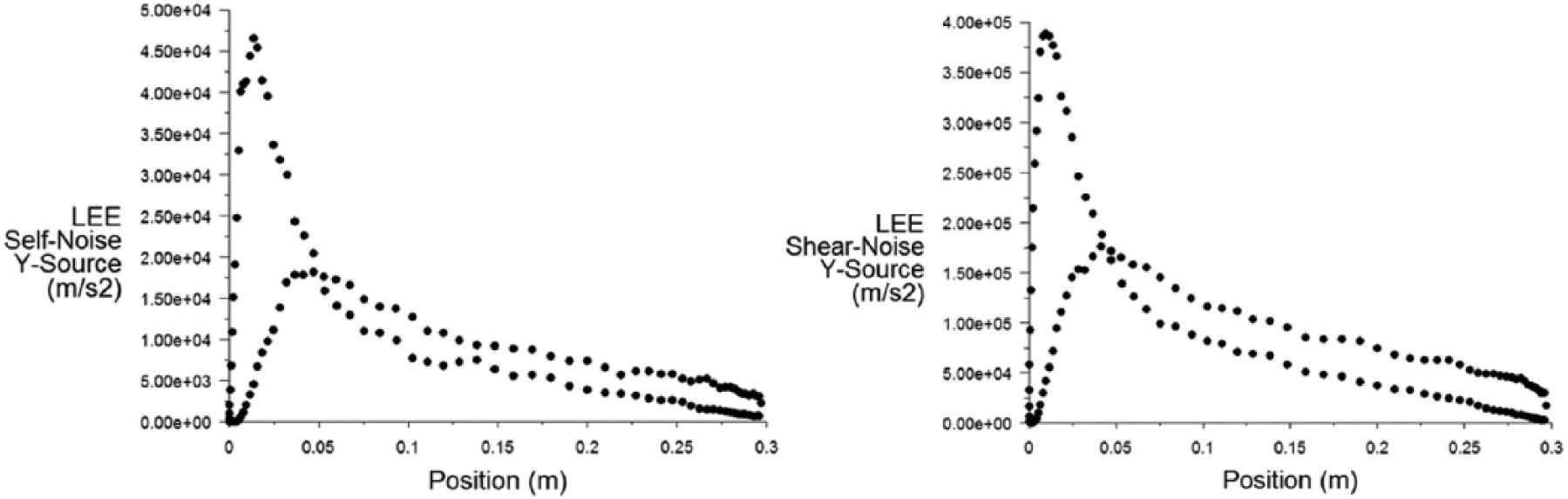
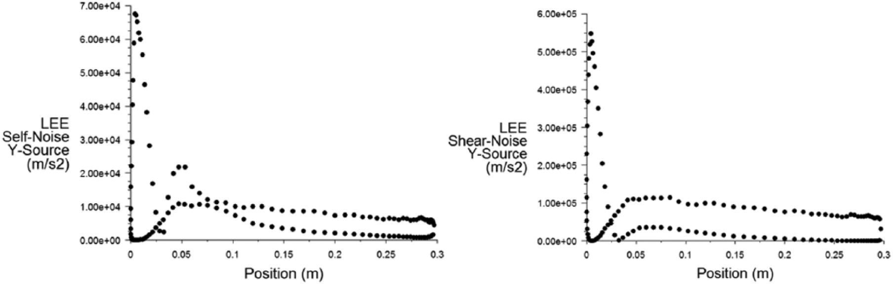
Graphs of y-directional noise sources (m/s²) across the airfoil profile for 16°, self-noise (left), and shear noise (right).

As for potential sources of error, section “CFD simulation” describes the methodology by which an accurate simulation environment has been created; the validation source in Figure 9 shows that the simulation has been performed with high accuracy.

Conclusion

Airfoil self-noise or trailing edge noise and shear noise were investigated computationally for a NACA0012 airfoil section, focusing on noise mechanisms at the trailing edge to identify and understand sources of noise production using ANSYS Fluent. A 2D CFD simulation has been performed for 0°, 8°, and 16° airfoil angles of attack capturing surface pressure contours, contours of turbulent intensity, contours of surface acoustic power level, vorticity magnitude levels across the airfoil profile, and x- and y-directional self-noise and shear noise sources across the airfoil profile. The results indicate that pressure gradients at the upper surface do increase as the angle of attack increases, which is a measure of vortices near the surface of the trailing edge associated with turbulence cease as the boundary layer begins to separate. Comparison of the turbulent intensity contours with surface acoustic power level contours demonstrated direct correlation between the energy contributed by turbulent structures (i.e. vortices) and the level of noise measured at the surface and within the boundary layer of the airfoil. As angle of attack is increased, both x and y sources have the same trends, yet, y sources (perpendicular to the free-stream flow) appear to have a bigger impact as angle of attack is increased. Furthermore, as the angle of attack increased, shear noise contributes less and less energy further downstream of the airfoil, and becomes dominated by noise energy from vortical structures within turbulence. The 2D CFD simulation revealed that pressure, turbulent intensity, and surface acoustic power contours further corroborated the previously tested noise observations phenomena reported by the authors at the trailing edge of the airfoil.

Footnotes

Acknowledgements

The research was conducted by B.R.J. in partial fulfillment of BSc (Hons) in Aerospace Technology at the Department of Engineering and Mathematics at Sheffield Hallam University under the supervision of Dr S.M.D.

Declaration of conflicting interests

The author(s) declared no potential conflicts of interest with respect to the research, authorship, and/or publication of this article.

Funding

The author(s) received no financial support for the research, authorship, and/or publication of this article.

References

Brooks

Pope

Marcolini

. Airfoil self-noise and prediction. Technical report, NASA reference publication 1218. Washington, DC: NASA, 1989.

Roger

Moreau

. Broadband self-noise from loaded fan blades. AIAA J 2004; 42(3): 536–544.

Roger

Moreau

. Trailing edge noise measurements and prediction for subsonic loaded fan blades. In: 8th AIAA/CEAS aeroacoustics conference & exhibit, Breckenridge, CO, 17–19 June 2002, AIAA paper no. 2002-2460.

Ffowcs Williams

Hall

. Aerodynamic sound generation by turbulent flow in the vicinity of a scattering half-plane. J Fluid Mech 1970; 40: 657–670.

Amiet

. Noise due to turbulent flow past a trailing edge. J Sound Vib 1976; 47: 387–393.

Howe

. A review of the theory of trailing edge noise. J Sound Vib 1978; 61: 437–465.

Brooks

Hodgson

. Trailing edge noise prediction from measured surface pressures. J Sound Vib 1981; 78: 69–117.

Jackson

Dakka

. An investigation into flow behavior and acoustic mechanisms at the trailing edge of an airfoil. Noise Vibr Worldw 2016; 47: 99–111.

Bardina

Huang

Coakley

. Turbulence modeling validation, testing, and development. San Jose, CA: NASA, http://www.ewp.rpi.edu/hartford/~ferraj7/ET/Other/References/nasa_techmemo_110446.pdf

10.

Menter

Kuntz

Langtry

. Ten years of industrial experience with the SST turbulence model. Otterfing: ANSYS-CFX, 2003.

11.

Marsden

Bogey

Bailly

. Direct noise computation around a 3-D NACA 0012 airfoil. Reston, VA: AIAA, 2006.