Noise source location and scaling of subsonic upper-surface blowing

Abstract

This paper deals with the topic of upper surface blowing noise. Using a model-scale rectangular nozzle of an aspect ratio of 10 and a sharp trailing edge, detailed noise contours were acquired with and without a subsonic jet blowing over a flat surface to determine the noise source location as a function of frequency. Additionally, velocity scaling of the upper surface blowing noise was carried out. It was found that the upper surface blowing increases the noise significantly. This is a result of both the trailing edge noise and turbulence downstream of the trailing edge, referred to as wake noise in the paper. It was found that low-frequency noise with a peak Strouhal number of 0.02 originates from the trailing edge whereas the high-frequency noise with the peak in the vicinity of Strouhal number of 0.2 originates near the nozzle exit. Low frequency (low Strouhal number) follows a velocity scaling corresponding to a dipole source where as the high Strouhal numbers as quadrupole sources. The culmination of these two effects is a cardioid-shaped directivity pattern. On the shielded side, the most dominant noise sources were at the trailing edge and in the near wake. The trailing edge mounting geometry also created anomalous acoustic diffraction indicating that not only is the geometry of the edge itself important, but also all geometry near the trailing edge.

Keywords

Jet noise airframe noise trailing edge noise noise source location

Introduction

Noise generated by upper-surface blowing is a problem relevant to several aerospace systems. In particular, over-the-wing engines and active flow control devices can generate substantial amounts of airframe noise due to higher velocity flow passing over aerodynamic surfaces, and upper-surface blowing. With these configurations providing context and motivation for the work presented, its relevance is drawn from the tightening airport noise regulations.

Most recently, there has been extensive work done to observe, develop theory, and model upper-surface blowing and jet-surface interaction by NASA Glenn Research Center.^1–12 From their work, it can be deduced that upper surface blowing has three primary noise sources, (1) jet noise, (2) surface scrubbing noise, and (3) trailing edge noise. At subsonic Mach numbers, trailing edge noise dominates.

The study of trailing edge noise dates back to the 1950s, and since then understanding has been gained about its generation and propagation. Much of this work has been summarized by Howe^13,14 and Doolan et al.^15–17 Relevant points from these papers, amongst other publications, are presented here to substantiate the findings of this paper.

What is known about subsonic trailing edge noise is that it is caused by a coupling of the hydrodynamic and acoustic fields,¹³ it has a broadband and tonal components,¹⁵ and that its directivity is a two-dimensional dipole.¹⁸ Although Ameit¹⁸ showed that trailing edge noise is generated by convection of unsteady pressure over the trailing edge, there are multiple theories about the pressure generation mechanism, the feedback path, and how they interact with the aerodynamic surface. The details are summarized below.

Howe¹⁴ and Ffowcs-Williams and Hall¹⁹ showed that when a dipole source interacts with an edge, a diffracted wave of opposite phase travels upstream toward the source of that dipole, and combines with subsequent downstream-propagating waves. The combination with downstream-propagating waves creates the feedback mechanism. Arbey and Bataille²⁰ suggest that unsteady pressure waves that convect downstream are hydrodynamic and originate at the maximum velocity location on the surface. The necessary condition is that the upstream propagating acoustic wave and the downstream convected hydrodynamic wave are phase-locked to establish a feedback path. Nakano et al.²¹ proposed a feedback mechanism similar to the former, except that the instability does not initiate from the point on the surface of maximum velocity, but rather the Tollmein-Schlichting (T-S) waves grow slowly over the surface and become large enough in amplitude to close the feedback loop before they reach the trailing edge. Nash et al.²² reiterate this theory. Tam and Ju²³ showed that the growth rate of T-S waves in the boundary layer are much too small to efficiently radiate this noise source, except for when the flow is separated. He suggests that the driver of this feedback mechanism is the instability of Kelvin-Helmholtz waves in the near wake, which propagate into the far-field and also interact with the trailing edge to energize the feedback mechanism. Chong and Joseph²⁴ were able to experimentally confirm that the feedback loop is closed by an upstream propagating acoustic wave, but determined that the mechanism is initiated at the point where the boundary layer instabilities originate, which could coincide with the point of maximum velocity or at the trailing edge, but does not have a deterministic location.

Desquesnes et al.²⁵ suggested that in addition to tones, when the flow becomes turbulent broadband noise is produced by chaotic hydrodynamic fluctuations. For sufficiently high Reynolds numbers for which the boundary layer becomes turbulent, the tones vanished.

Despite there being many theories regarding the feedback mechanism and trailing edge noise location of origin, it is clear that all proposed mechanisms contain many similarities including, fluctuating pressure waves over the surface that are convectively amplified in the vicinity of the trailing edge.

This research attempts to expand on the classical works published by Brooks and Pope,²⁶ Brooks and Hodgson,²⁷ and Hutcheson and Brooks²⁸ by examining trailing edge noise using upper-surface blowing. To control subsonic upper-surface blowing noise, it is important to first understand where this noise originates and how it scales with velocity. Experiments were conducted at several subsonic Mach numbers to determine the noise source location and scaling. Additionally, a simple iterative method for correcting near-field acoustic measurements will be described and employed.

Experimental procedure

The Huie-Songer Small-Scale Aeroacoustic Flow Visualization Laboratory at the Georgia Tech Research Institute (GTRI), Cobb County was used to conduct these experiments. The facility is a 24′ × 10′ × 8′ partially-treated room with 6″ thick concrete walls downstream of the rig and sheet-rock walls upstream of the rig, and a similar ceiling. The facility has been outfitted with 18″ melamine foam wedges, making it anechoic above 400 Hz. The average noise floor between 0.4 and 50 kHz is 30 dB in this facility. The facility is equipped with a 3-axes traverse, ambient pressure temperature and humidity sensors, PCB Peizoelectronics 378C01 1/4″ microphone, and National Instruments USB-4431 data acquisition system sampling at 102 kHz. An additional PCB Peizoelectronics 378C01 1/4″ microphone is mounted above the nozzle at (1.5′, 1.5′, 0′) from the jet exit. This microphone is intended to identify run-to-run variations in SPL’s while acquiring acoustic measurements. The other microphone is mounted to the traverse and is used to perform near-field acoustic surveys. A schematic of the facility is seen in Figure 1.

Figure 1.

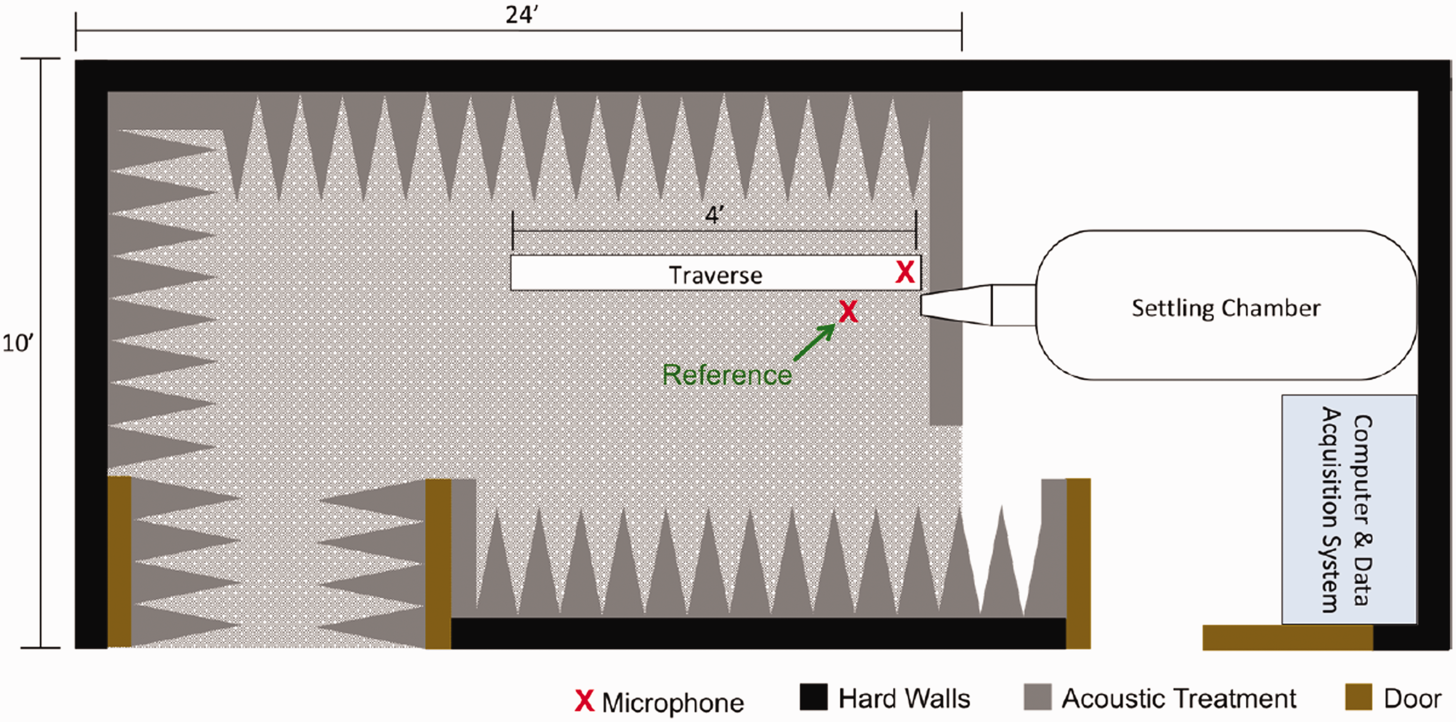
Top-view schematic of the Huie-Songer Small-scale Aeroacoustic Flow Visualization Laboratory at GTRI, Cobb County (not to scale).

Two aspect ratio (AR) = 10 (D_eq = 3/4″) converging, rectangular nozzles were used in this study. One is designed to conduct isolated jet experiments, and another for upper-surface blowing experiments. As seen in Figure 2, the upper-surface blowing configuration flush-mounted the rectangular nozzle with an 8″ long steel plate and 3-D printed Polylactic Acid (PLA) 1.5″ long, 1/20″ thick sharp trailing edge. L/h = 45 for this configuration.

Figure 2.

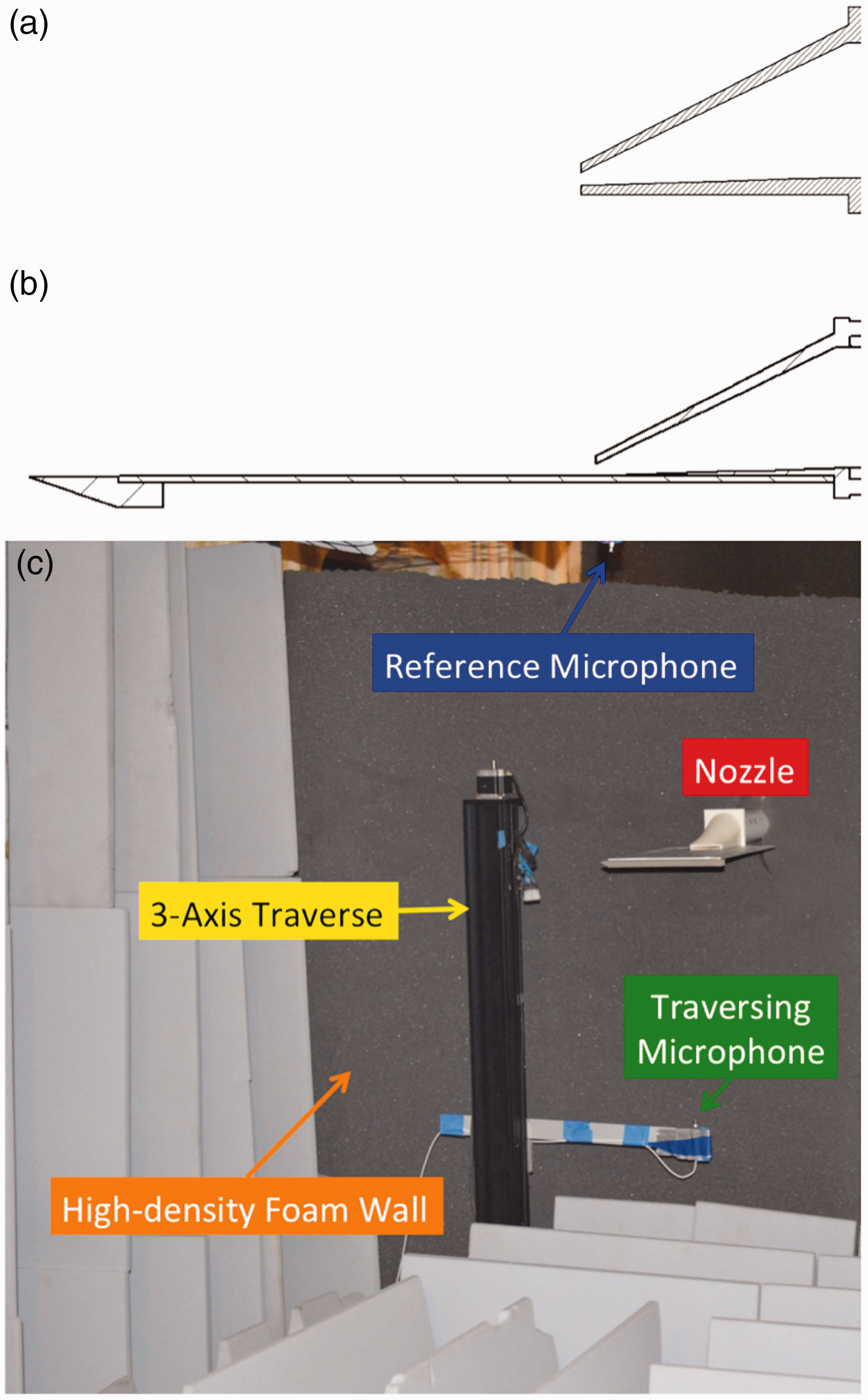
(a) AR = 10, converging rectangular nozzle used for isolated jet experiments, (b) nozzle with flush-mounted steel surface and sharp trailing edge and (c) nozzle mounted with surface and trailing edge in testing facility.

Unheated experiments were conducted for both configurations at jet ambient Mach numbers between 0.4 and 0.8. Measurements at each location were taken for 15 seconds. The sample period was selected such that a large number of samples could be used when processing data into the frequency domain, and improve measurement accuracy. Experimental trials were repeated to further ensure the accuracy of the measurements. During each measurement, ambient pressure and temperature, plenum pressure and temperature, acoustic pressure, and humidity signals were recorded. Microphone data was processed in narrowband (Δf = 16 Hz) between 0.4 and 50 kHz. The reference coordinate system is seen in Figure 3. 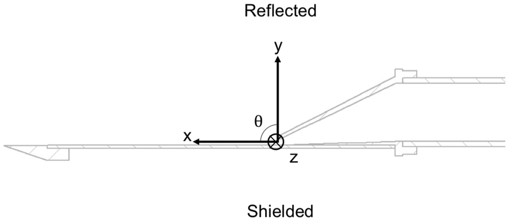The angle θ is defined as rotation about the z-axis, and $ϕ$ is defined as rotation about the y-axis. Positive angles of rotation are in the counter-clockwise direction.

Figure 3.

Diagram showing the coordinate system used in acoustic surveys.

The reflected side and shielded side denote above and below the surface, respectively. The terms “Reflected “and “Shielded “will be used to refer to microphones associated with these regions of measurements. All measurements were corrected for atmospheric attenuation, the free-field response of the microphone, and the incidence angle of sound from each calculated source on the microphone. The reference pressure in sound pressure level (SPL) calculations was 20 μPa.

To create noise contours, a microphone traversed an equally-spaced Cartesian grid of the noise field but outside the hydrodynamic field. The resolution of the grid was 1″ in the x and y-coordinate directions. All points in the grid were measured in succession, causing the run time of an acoustic survey to be roughly 2 hours. Fluctuations in jet Mach numbers were ±0.005 over a single survey. By taking a Fourier transform of each sample, the spatial distribution of SPL as a function of amplitude was be realized. Noise source locations were computed by analyzing each frequency individually. The process involved locating the point of maximum amplitude in the measured acoustic field. The spatial gradient of SPL was calculated about the maximum amplitude point, by the 5-point central differencing scheme. The gradient vector was then used to locate the source by assuming that it landed along the jet center axis. A limitation of this method is that only the loudest source is captured.

Without further processing, the noise source location approach disregards the effects of wave incidence and atmospheric attenuation on the source amplitude and location. To present a correct noise source location curve, a methodology for applying corrections needed to be developed. The source location and acoustic corrections are fully-coupled and must be converged simultaneously. The process used to apply corrections to the data and generate the source location curves can be seen in Figure 4.

Figure 4.

Flowchart of process used to apply corrections to noise contours and generate noise location curves.

To describe the process employed, uncorrected noise spectra were first processed using the Matlab wavelet denoising function wden. To do so, 5 levels of Morlet wavelets were used. This technique was leveraged to overcome the fact that the facility used was not fully treated for acoustic absorption. Using these filtered signals, the noise source location curve is generated using the process described above. Using this initial source location curve, corrections were applied for microphone free-field response, wave incidence, and atmospheric attenuation. The source location of each frequency in the curve was then compared with the previous iteration to determine if convergence was achieved, and iteration continued.

Results

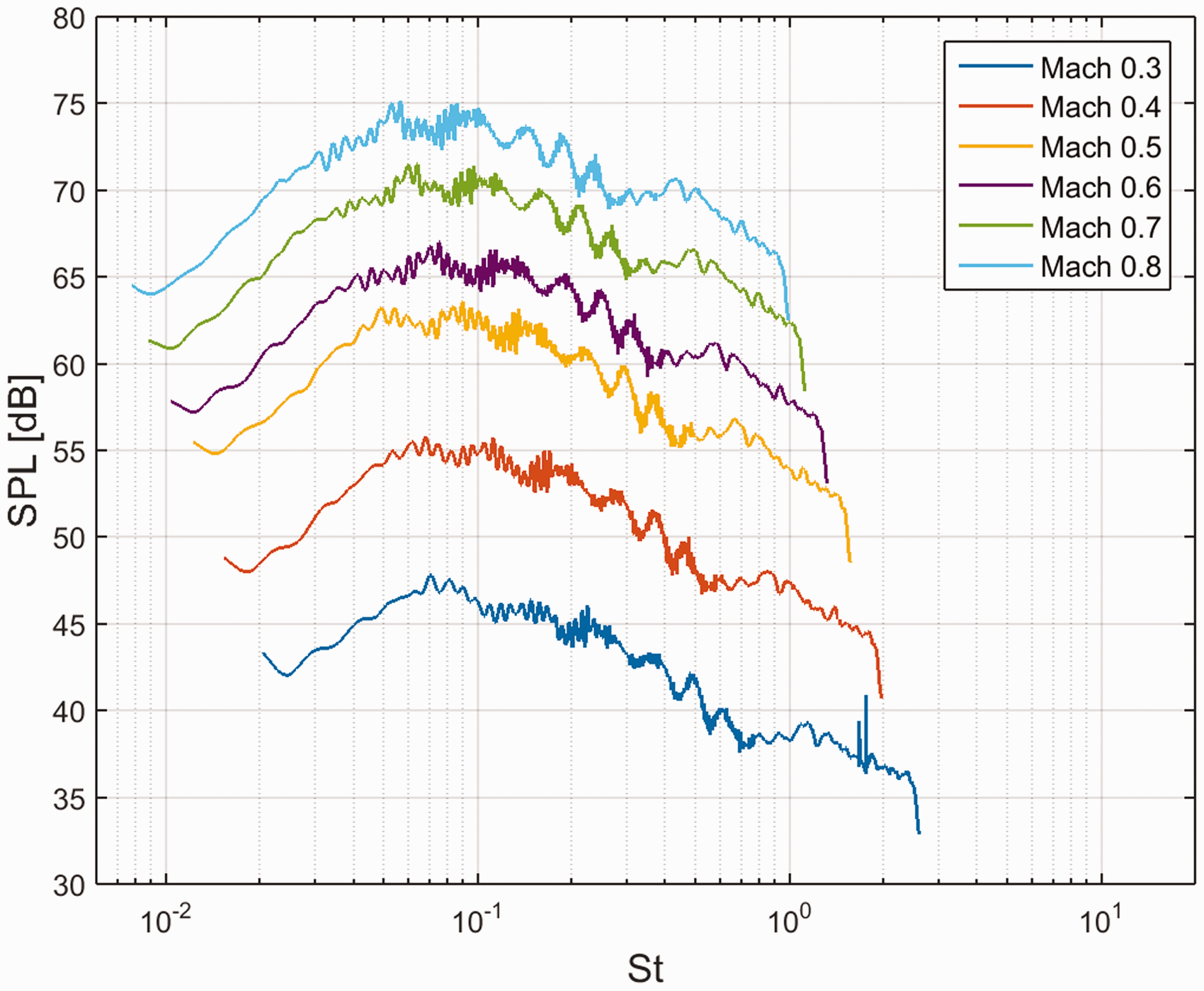
The rectangular jet was characterized first, to quantify the effect of adding the surface and trailing edge. Acoustic spectra of the isolated jet were computed, and are shown in Figure 5. In this figure jet Mach number is defined as $U_{j} / a_{0}$ , and R/h is the non-dimensional distance from the nozzle exit plane. Two distinct peaks were seen in the spectra, and are attributed to the 10:1 aspect ratio of the jet. The two peaks are formed because the width is an order of magnitude greater than the height, causing the mixing layer to be much thicker along the major axis and causing an offset in peaks.

Figure 5.

Near-field noise spectrum for isolated AR = 10 (D_eq = 3/4″) jet at $U_{j} / a_{0}$ = 0.3–0.8, θ = 90°, and R/h = 70.

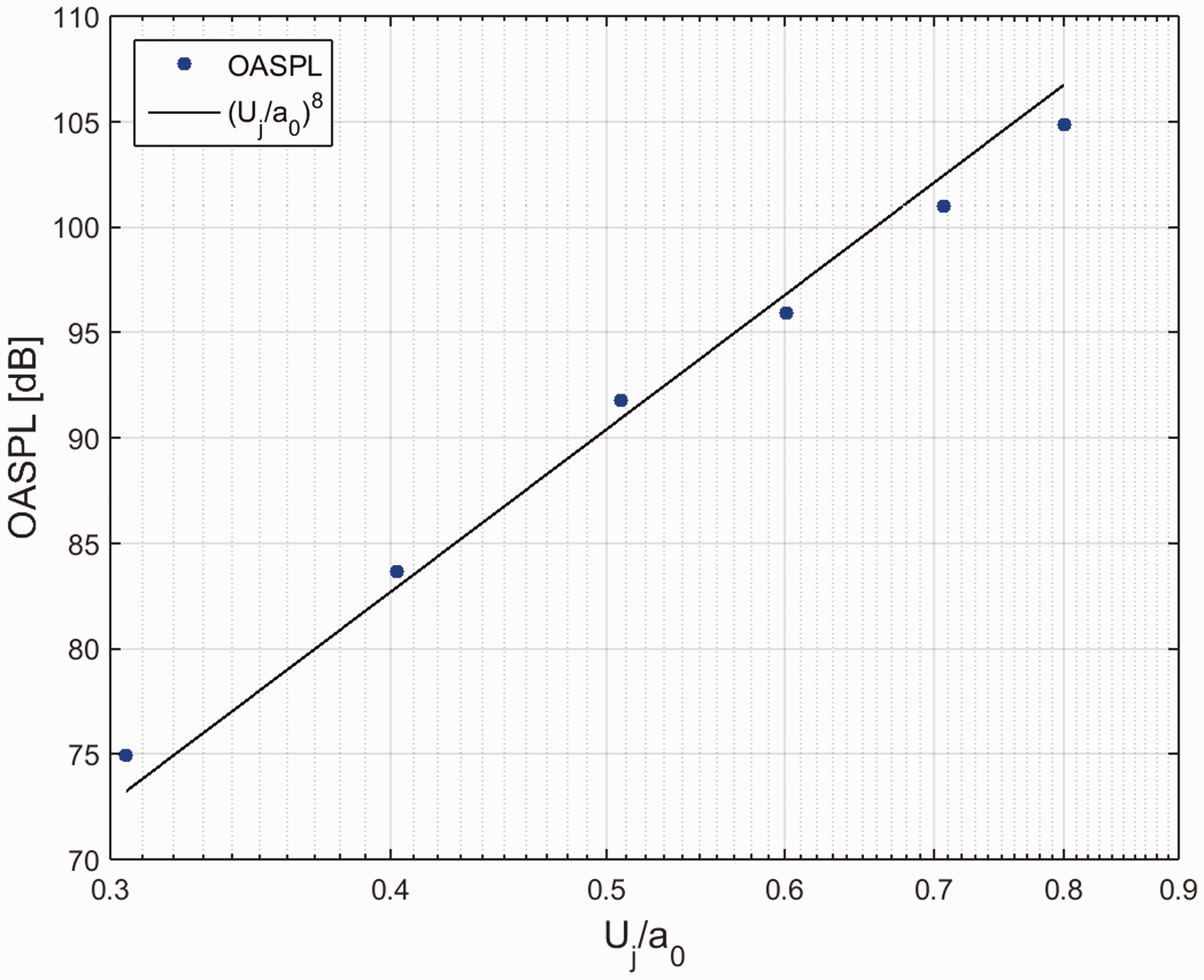
Additionally, the OASPL was calculated for Mach numbers between 0.4 and 0.8, and the noise follows ${(U_{j} / a_{0})}^{8}$ scaling and concludes that the nozzle is producing typical jet noise. Figure 6 shows the OASPL scaling of the isolated jet used in these experiments.

Figure 6.

OASPL scaling of AR = 10 rectangular jet from near-field spectra at $U_{j} / a_{0}$ = 0.3–0.8, θ = 90°, and R/h = 70.

By adding a surface under the jet, changes in the spectra were found, and are illustrated in Figure 7. When considering the orientation of the observer, it is clear that at the sideline position, there is no low Strouhal number (St = ∼0.02) hump, which is seen in the reflected and shielded near-field noise spectra of Figure 7. The hump of is of approximately the same amplitude at both orientations. This supports the 2 D, dipole nature of trailing edge noise discribed by Amiet.¹⁸ The shielded side of the surface shows much lower noise at high Strouhal numbers (St > 0.04), than the reflected side, which confirms that high-frequency noise comes predominantly from the region over the surface, and is likely jet mixing noise produced over the surface.

Figure 7.

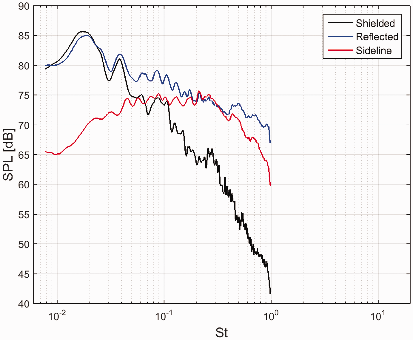
Comparison of near-field noise spectra recorded at θ = 90°, R/h = 70 and $U_{j} / a_{0}$ = 0.8 in the reflected, shielded and sideline planes with respect to the jet center axis and L/h = 45 surface attached.

In Figure 8, the reflected and shielded side spectrum are compared with a spectrum of the isolated jet. At Strouhal numbers greater than 0.04, there is a 3 dB difference between the SPL of the reflected spectrum and the isolated jet spectrum. This implies that the noise is “doubled “by the jet mixing noise reflecting off the surface, and doing so in an incoherent manner.

Figure 8.

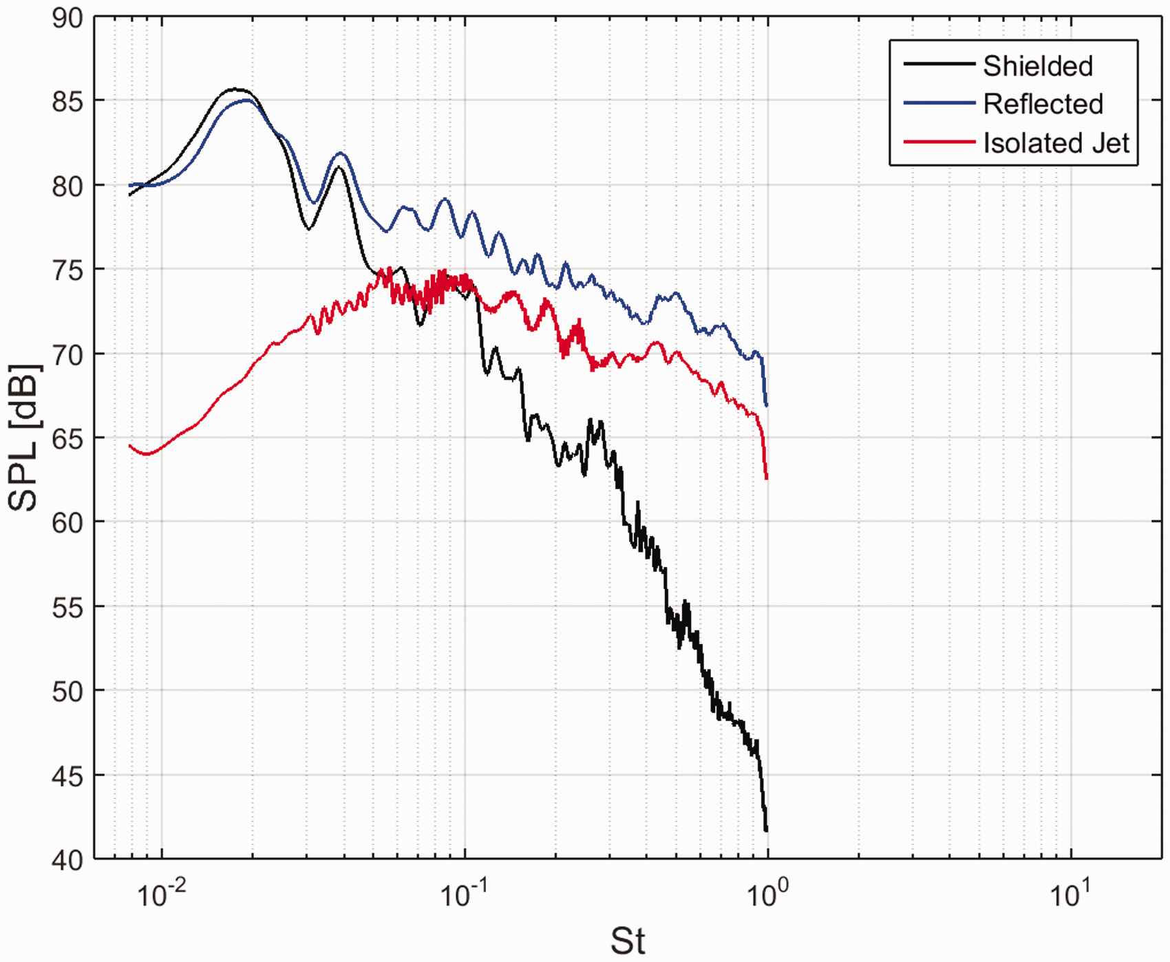
Comparison of near-field noise spectra recorded at θ = 90°, R/h = 70 and $U_{j} / a_{0}$ = 0.8 in the reflected, shielded planes with an isolated rectangular jet of the same dimensions.

Noise source scaling

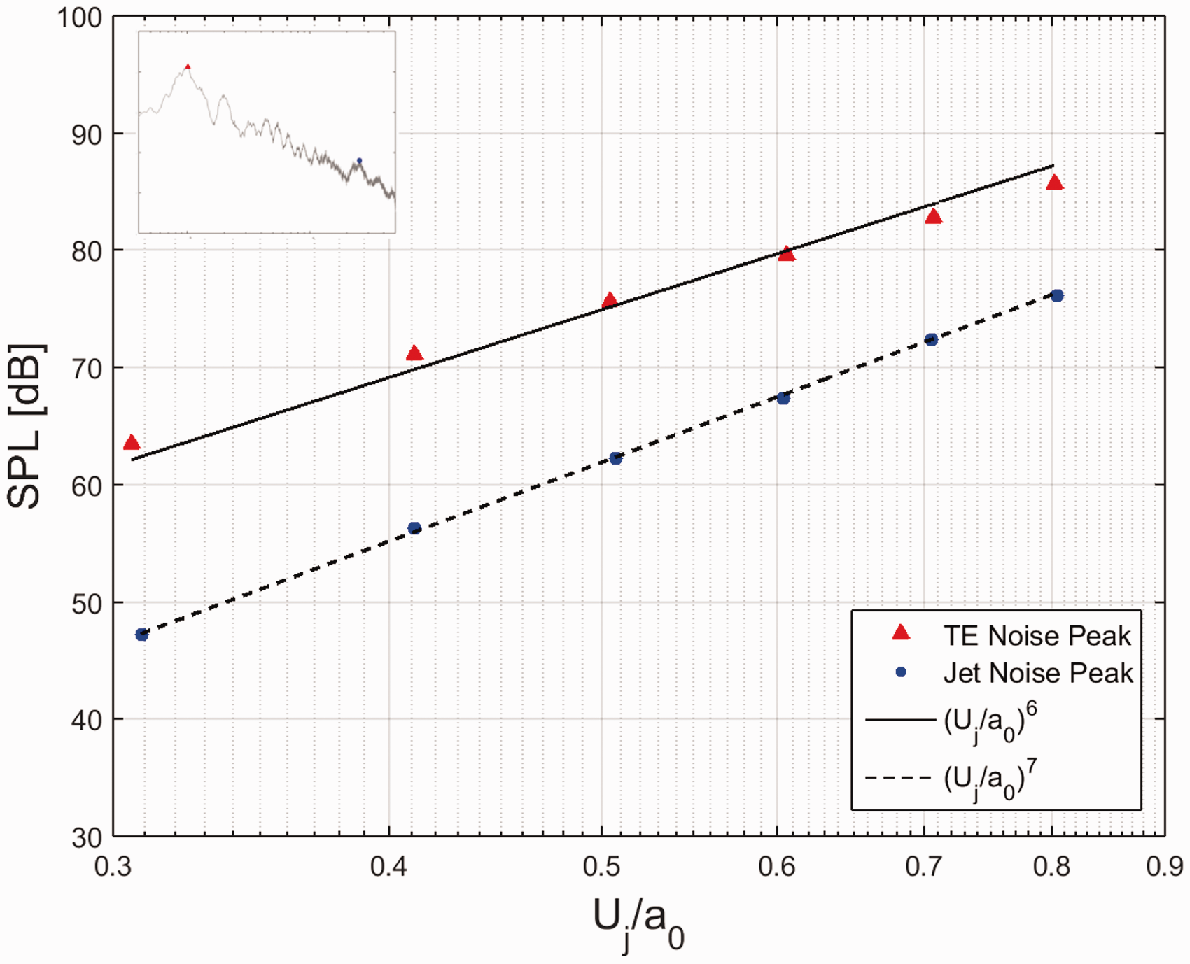
As seen in Figure 9, the scaling of the low frequency (TE noise) and high frequency (jet-mixing noise) peaks follow ${(U_{j} / a_{0})}^{6}$ and ${(U_{j} / a_{0})}^{7}$ , respectively. Low and high frequency peaks of a typical spectrum can be seen in the upper left corner of the figure. By comparison with Lighthill’s acoustic analogy, where dipole sources scale as ${(U_{j} / a_{0})}^{6}$ and quadrupole sources scale as ${(U_{j} / a_{0})}^{8}$ , it appears that the low and high frequency peaks may behave as dipole noise and quadrupole sources, respectively. Additionally, the difference between what is believed to be the trailing edge and jet noise peaks varies from 10–15 dB between Mach = 0.4 and Mach = 0.8. This reiterates the strength of the trailing edge noise, as it dominates the acoustic signature for the geometry studied.

Figure 9.

Trailing edge and jet noise peak scaling vs. jet Mach number from near-field spectrum, θ = 90° and R/h = 70.

Noise source location

Figure 10 depicts the acoustic near-field and noise location at various frequencies, which were selected based on peaks seen in the far-field noise spectrum at $U_{j} / a_{0} = 0.6$ . The reflected side is in the positive y/h direction, and the nozzle exit plane resides at $x / h = 0$ .

Figure 10.

Noise contours of SPL (in dB) on 8″ surface with 1.5″ sharp trailing edge attached at $U_{j} / a_{0}$ = 0.6, where the dotted line indicates the streamwise position of the trailing edge.

At the trailing edge and in the near wake, noise of significant amplitude can be seen across all frequencies in Figure 10, even at St > 0.2 where jet noise is generally more dominant. Additionally, contributions to the low-Strouhal number (St = 0.02) hump are coming from over the surface, on the reflected side. This could be partly due to turbulent scattering in the surface boundary layer or scrubbing noise directly. Evidence of this is seen in the 944 Hz and 1520 Hz contour plots of Figure 10, as there are significant amounts of noise generated over the surface and in the wake. It was also proved that this contribution could not be from jet-mixing noise as it was shown in Figure 8 that the isolated jet is of relatively low amplitude at this Strouhal number. This observation supports the claims of Tam, that the noise can be generated both at the trailing edge and in the near wake.²³

On the reflected side of the surface is seen in Figure 10, noise is to be radiating in two separate directions. It is believed that there are two distinct sources causing this noise which are (1) jet mixing noise being reflected normal to the surface and (2) traditional subsonic jet noise propagating downstream. This can be verified by the spectra in Figure 8, where the far-field noise on the reflected side is 3 dB higher than the isolated jet. It is also known that jet noise reaches its peak amplitude at low angles of θ.

At St > 0.2, the geometry used to attached the trailing edge on the shielded side is creating anomalous acoustic diffraction. This shows that not only is the geometry of the edge itself is important, but also all geometry in the vicinity of the trailing edge. This finding provides an area of opportunity for control of trailing edge noise, and upper-surface blowing noise alike.

Further insight can be gained by inspecting the source location curves in Figure 11. As seen in other literature,²⁹ the jet noise sources begin at the jet exit. From the nozzle exit, high-frequency sources cascade into lower frequency sources downstream. On the reflected side of the surface, the same can be seen. With the high-frequency sources near the jet exit, they are blocked from an observer on the shielded side of the surface.

Figure 11.

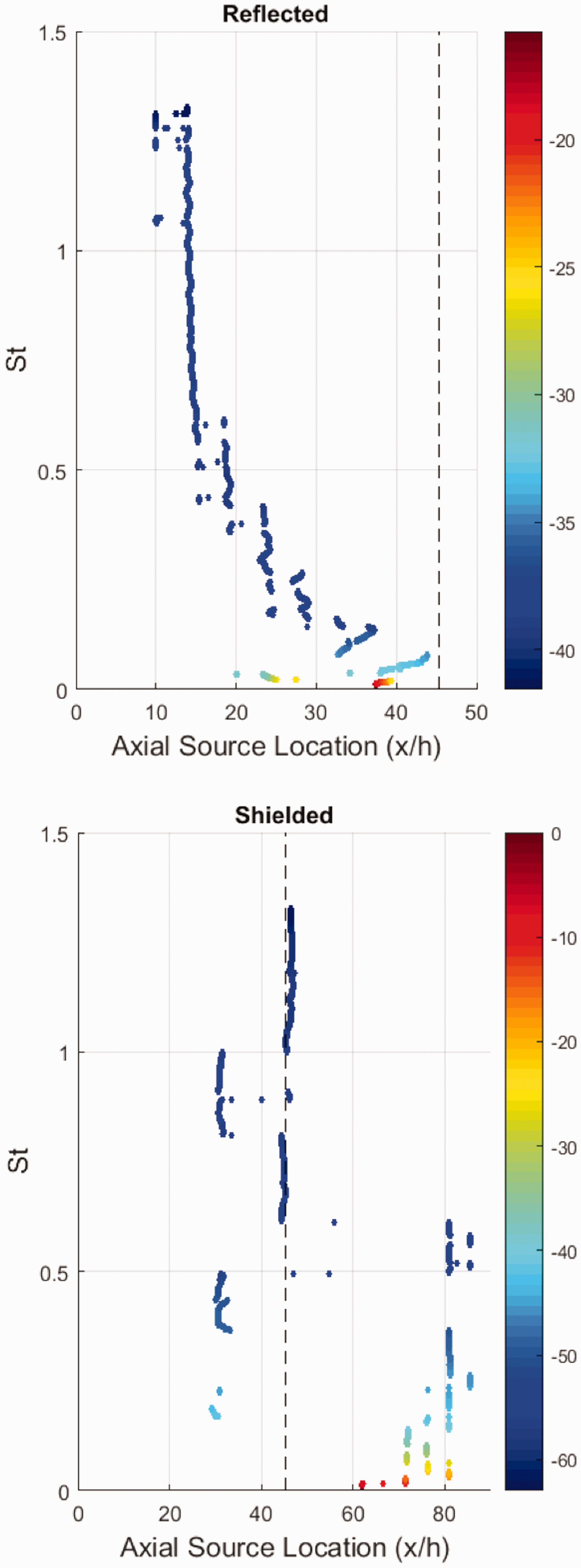
Noise source location curves computed from reflected and shielded side noise contours for a $U_{j} / a_{0}$ = 0.6 with 8″ surface and 1.5″ sharp trailing edge attached.

In addition to the jet-like source curve, a second source curve begins at about the mid-chord of the surface that is consistently at low Strouhal number, high amplitude, and terminates in the near wake, when observing from the reflected side. Since the second source occurs at almost consistently at low Strouhal number, the theory regarding the growth of waves over the surface that convect about the trailing edge is believed to be shown here.

On the shielded side of the surface, it is seen that all sources originate at the trailing edge of the surface or in the near wake. As mentioned previously, some sound diffracts about the trailing edge attachment geometry, rather than the edge itself. It is believed that if the geometry/method used to mount the surface were done in such a way that there were no sharp edges (besides the trailing edge itself), all sources would fall in an approximately straight line at the trailing, with some sources scattered in the near wake.

Near-field directivity

OASPL was computed for polar angles between − $180$ ° and $180$ ° with respect to the trailing edge and are displayed in Figure 12 it is depicted that noise creates a cardioid shape about the trailing edge, further reinforcing the dipole nature of trailing edge noise. This also reiterates that the trailing edge noise component dominates upper-surface blowing noise between jet Mach numbers of 0.4 and 0.8.

Figure 12.

Directivity of OASPL about the trailing edge for R/h = 230 and $U_{j} / a_{0}$ = 0.6.

Source location and amplitude correction

The purpose of this section is to depict the importance of correction for near-field microphone data. Correction of the acoustic signals was done in the frequency-domain using data and can be seen in Figures 13 and 14. it was assumed that all sources occur along the jet axis, and movement of each source, and its associated amplitude, between the first and last iterations of the correction process were plotted. The changes in noise source location and amplitude are shown to be significant at St > 0.1.

Figure 13.

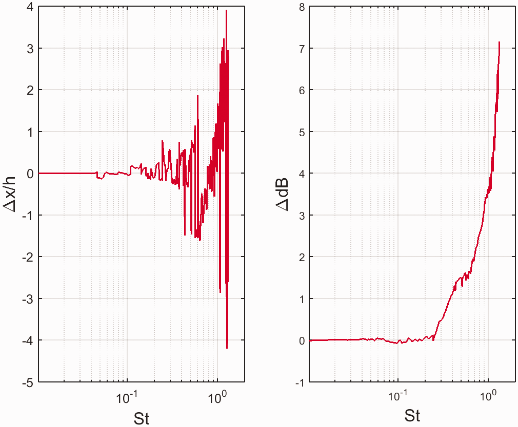
Change in source location and amplitude vs. frequency between first and last iterations on the reflected side of the surface with the sharp trailing edge attached.

Figure 14.

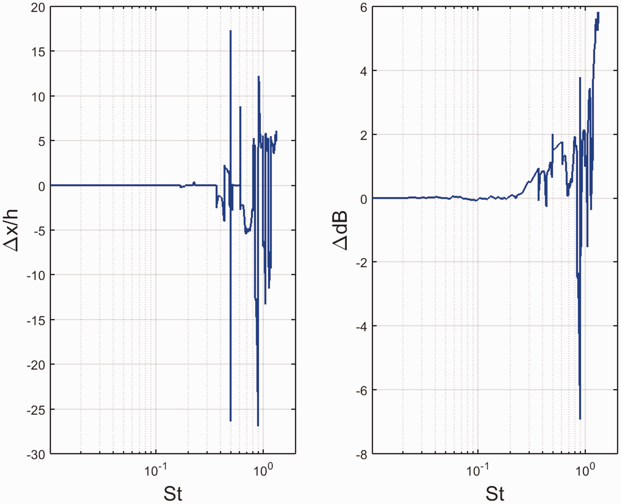
Change in source location and amplitude vs. frequency between first and last iterations on the shielded side of the surface with the sharp trailing edge attached.

The largest source location deviation was 27 nozzle heights, or 60% of the exhaust surface length. This correction method also had an impact on the SPL, with the largest change in amplitude being 7 dB. These results show that atmospheric attenuation and microphone response play a major role in noise source location measurement especially at high frequencies, when using a traversing microphone.

Summary

The authors’ literature survey did not find a study that examined noise contours of an upper-surface blowing configuration, and such measurements became the backbone of this study. Extensive noise contours were made on both the reflected and shielded side of the configuration and reveal that both the trailing edge and wake produce additional noise over that of an isolated jet.

At low (0.02) and high (0.2) Strouhal number peaks follow ${(U_{j} / a_{0})}^{6}$ and ${(U_{j} / a_{0})}^{7}$ , respectively. These are believed to be the trailing edge and jet noise peaks, respectively. The difference between the trailing edge and jet noise peaks varies from 10–15 dB over the range studied, thus showing the dominance of a trailing edge noise component.

The noise contours show that significant noise is generated in the vicinity of the trailing edge at all Strouhal numbers. Additionally, there is noise of significant amplitude in the wake and over the surface. At Strouhal number greater than 0.2 on the reflected side, noise is shown to radiate in two separate directions on the reflected side of the surface. It is believed that there are two distinct sources causing this noise which are (1) jet mixing noise being reflected normal to the surface and (2) traditional subsonic jet noise propagating downstream. This can be verified by the spectra in Figure 8, where the far-field noise on the reflected side is 3 dB higher than the isolated jet. On the shielded side, the most dominant noise sources were at the trailing edge and in the near wake. The trailing edge mounting geometry created anomalous acoustic diffraction. This shows that not only is the geometry of the edge itself is important but also all geometry in the vicinity of the trailing edge, and could be a location for a noise control device.

This work displays the dominance of the trailing edge in upper-surface blowing noise at subsonic conditions. Although it is less sensitive to velocity, its larger amplitude does not allow the jet noise component to overcome it. Such findings can support the development of techniques and methodologies that reduce the noise source, without prescribing modifications to the edge itself, and ultimately increasing the number of noise control mechanisms.

Footnotes

Acknowledgements

The authors would like to thank the Georgia Tech Research Institute for the use of their facilities, instrumentation, and technical expertise. The authors are particularly grateful to Graduate Student Nick Breen for allowing the use of his microphone traverse and related noise analysis programs.

Declaration of conflicting interests

The author(s) declared no potential conflicts of interest with respect to the research, authorship, and/or publication of this article.

Funding

The author(s) received no financial support for the research, authorship, and/or publication of this article.

ORCID iD

Trae L Jennette

References

Bridges

Noise from aft deck exhaust nozzles – differences in experimental embodiments. In: 52nd aerospace sciences meeting, National Harbor, MD, 13–17 January 2014.

Brown

CA.

Developing an empirical model for jet-surface interaction noise. In: 52nd aerospace sciences meeting, National Harbor, MD, 13–17 January 2014.

Brown

CA.

An Empirical jet-surface interaction noise model with temperature and nozzle aspect ratio effects. In: 53rd AIAA aerospace sciences meeting, Kissimmee, FL, 5–9 January 2015.

Brown

CA.

Empirical models for the shielding and reflection of jet mixing noise by a surface. In: 21st AIAA/CEAS aeroacoustics conference, Dallas, Texas, 22–26 June 2015.

Brown

CA.

Including finite surface span effects in empirical jet-surface interaction noise models. In: 54th AIAA aerospace sciences meeting, San Diego, CA, 4–8 January 2016.

Brown

Clem

Fagan

AF.

Investigation of broadband shock noise from a jet near a planar surface. J Aircraft 2015; 52: 266–273.

Brown

Wernet

Jet-surface interaction test: flow measurement results. In: 20th AIAA/CEAS aeroacoustics conference, Atlanta, GA, 16–20 June 2014.

Clem

Brown

Fagan

AF.

Background oriented Schlieren implementation in jet-surface interaction test. In: 51st AIAA aerospace sciences meeting, Dallas/Ft. Worth, TX, 7–10 January 2013.

Khavaran

Acoustics of jet surface interaction – scrubbing noise. In: 20th AIAA/CEAS aeroacoustics conference, Atlanta, GA, 16–20 June 2014.

10.

Khavaran

Bozak

Brown

CA.

Jet surface interaction noise in a planar exhaust. In: 22nd AIAA/CEAS aeroacoustics conference, Lyon, France, 30 May–1 June 2016.

11.

Zaman

KBMQ

Fagan

Bridges

, et al. Investigating the feedback path in a jet-surface resonant interaction. In: 21st AIAA/CEAS aeroacoustics conference, Dallas, TX, 22–26 June 2015.

12.

Zaman

KBMQ

Fagan

Clem

, et al. Resonant interaction of a rectangular jet with a flat-plate. In: 52nd aerospace sciences meeting, National Harbor, MD, 13–17 January 2014.

13.

Howe

MS.

A review of the theory of trailing edge noise. J Sound Vibr 1978; 61: 437–465.

14.

Howe

MS.

Hydrodynamics and sound. New York: Cambridge University Press, 2006.

15.

Doolan

CJ.

A review of airfoil trailing edge noise and its prediction. Acoustics Australia 2008; 36: 7–13.

16.

Doolan

Brooks

LA.

A review of trailing edge noise generated by airfoils at low to moderate Reynolds number. Acoustics Australia 2011; 38: 135–139.

17.

Doolan

Moreau

DJ.

A review of airfoil trailing edge noise with some implications for wind turbines. Int J Aeroacoust 2015; 14: 811–832.

18.

Amiet

RK.

Noise due to turbulent flow past a trailing edge. J Sound Vibr 1976; 47: 387–393.

19.

Williams

JEF

Hall

LH.

Aerodynamic sound generation by turbulent flow in the vicinity of a scattering half plane. J Fluid Mech 1970; 40: 657–670.

20.

Arbey

Bataille

Noise generated by airfoil profiles placed in a uniform laminar flow. J Fluid Mech 1983; 134: 33–47.

21.

Nakano

Fujisawa

Lee

Measurement of tonal-noise characteristics and periodic flow structure around NACA0018 airfoil. Exp Fluids 2006; 40: 482–490.

22.

Nash

Lowson

McAlpine

Boundary-layer instability noise on aerofoils. J Fluid Mech 1999; 382: 27–61.

23.

Tam

CKW

Aerofoil tones at moderate Reynolds number. J Fluid Mech 2012; 690: 536–570.

24.

Chong

Joseph

An experimental study of tonal noise mechanism of laminar airfoils. In: 30th AIAA aeroacoustics conference. AIAA, Miami, FL, 11–13 May 2009.

25.

Desquesnes

Terracol

Sagaut

Numerical investigation of the tone noise mechanism over laminar airfoils. J Fluid Mech 2007; 591: 155–182.

26.

Books

Pope

DS.

Airfoil self-noise and prediction. NASA Reference Publication 1218, 1989.

27.

Brooks

Hodgson

TH.

Trailing edge noise prediction from measured surface pressures. J Sound Vibr 1981; 78: 69–117.

28.

Hutcheson

Brooks

TF.

Effects of angle of attack and velocity on trailing edge noise. Int J Aeroacoust 2006; 5: 39–66.

29.

Breen

Ahuja

KK.

Jet noise source location by acoustic beamforming and nearfield sound contours – a comparison. In: 23rd AIAA/CEAS aeroacoustics conference, AIAA, Denver, Colorado, 5–9 June 2017.