Rolling element bearing fault detection based on the complex Morlet wavelet transform and performance evaluation using artificial neural network and support vector machine

Abstract

Condition monitoring and fault diagnosis of rolling element bearings are very important to ensure proper working of different types of machinery. Condition monitoring of rotating machines is mainly based on the analysis of machine vibration. The vibration signals from the mechanical fault generally comprise periodic impulses with specified characteristic frequency corresponds to a particular defect. But due to heavy noise in the industry, the vibration signals have a very low signal-to-noise ratio. Hence, it requires an appropriate technique to extract the impulses from the noisy signal. This article emphasized on the fault diagnosis of rolling element bearings having some specific size of defects on various bearing elements using the complex Morlet wavelet analysis. The phase and amplitude map of the complex Morlet wavelet are utilized for identification and diagnosis of the fault in the rolling element bearing. The amplitude and phase map corresponding to the complex Morlet wavelet are found to show unique informative signatures in the presence of bearing faults. The classification technique based on artificial neural network and support vector machine for rolling element bearing fault detection is presented in this article. The classification results of bearing faults clearly indicate that support vector machine has a more precise bearing fault classification ability than artificial neural network.

Keywords

Condition monitoring rolling element bearing fault diagnosis support vector machine artificial neural network

Introduction

Bearings are important elements in rotary machines due to their friction-reducing and load-bearing capacity. The rolling element bearing is an important component of the power transmission system. Machine performance is greatly influenced by the operating condition of the rolling element bearing. Proper functioning of machinery depends, to a great extent, on early detection of bearing fault. If not detected in time, the bearing defect would cause a malfunction that may even lead to sudden failure of the machinery. Hence, the proper condition monitoring of the bearing components gives a better advantage in the operation and maintenance field, which leads to a safe working environment. Therefore, the fault detection of rolling element bearings at the early stage of propagation has been the subject of extensive research. The general industrial philosophy of utilizing vibration data and signal as a source of machine condition information to minimize maintenance and operating costs and making the machine available in healthy condition is the point of extensive research in the process industry. The most common and reliable method to observe the machine condition is to analyze the vibration data and signature. In recent decades, the researchers have begun using many techniques such as optimal wavelet filter-based method, spectral kurtosis, and high-frequency resonance technique for the fault diagnosis and analysis of rolling element bearing.

The rolling element bearings are subjected to massive loads under different operating conditions in the process plant. Due to these loadings, wear, spall, or pitting may appear on the bearing after a long period of use.¹,² The components that are subjected to failure in a rolling element bearing are inner race, outer race, and balls. The traditional method of machine fault detection is to look for a peak at characteristic defect frequency in the frequency domain. However, it is not feasible to detect the bearing fault in the traditional manner as a series of impact vibrations are generated by bearing defects whenever a moving ball crosses over the surface of the defect.^1,3–6 The resultant vibration in the time domain is characterized by sharp peaks and the energy from these sharp impact vibrations is distributed over a wide frequency range. Generally, low energy is associated with the frequency of defective bearing, and hence, it can be easily covered by other low-frequency effects and noise.^7–12

The time and frequency domain techniques have been developed by the researchers to overcome these problems. They have developed some techniques which generally use some parameters that are sensitive toward impulse oscillations, such as crest factor, kurtosis, peak level, root mean square (RMS) value, and shock pulse.^13–15 The passage of the rolling element over the fault causes an impact due to a sudden change of contact stresses. This excites one or more resonant frequencies of the bearing. Typically, the resonant frequencies lie in the high-frequency range, which is more than 5 kHz. Hence, many techniques that employ high-frequency vibrations in various ways have been developed for bearing fault detection.¹⁶ However, all these techniques are not able to detect the bearing faults with high success especially when the defect is at the early stage. In recent years, soft computing has made great progress and has been applied effectively for machinery fault detection. Various researchers have applied artificial neural networks (ANNs) for the detection of rolling element faults. Support vector machine (SVM) is another potential classification technique that has been used effectively for bearing fault detection and classification.^10,17 As both of these algorithms have been used effectively for bearing fault detection and classification, a comparative study of ANN and SVM has been done in this article to identify the best method.

The wavelet transform is a most adorable tool, because of its multi-resolution analysis capability in both time and frequency domains. Hence, it is widely used by the researchers and the maintenance persons in the process industry, for the extraction of the informative characteristic features from non-stationary vibration signature generated by the defective bearing.¹⁸,¹⁹ A series of wavelet coefficients are generated by the wavelet analysis techniques, which clearly depict that how far the signal is to the particular wavelet. A suitable wavelet base function should be adopted to extract the fault characteristic of the signal more fruitfully. The impulse signal generated by the faulty rolling element bearing is having a greater extent of similarity with the Morlet wavelet. Hence, it is mostly used to extract the fault feature of rolling element bearing. Then the response wavelet is constructed and it is implemented to draw out the characteristic feature of the vibration signal by the faulty bearing.²⁰,²¹

In the present work, the vibration signatures were extracted from standard new bearing in normal working condition and from faulty bearings with some artificially induced faults. Features are obtained from vibration signals of bearing running in good and faulty conditions. These features are taken as input parameters to the ANN and SVM classifier to train these classifiers to distinguish features of good bearing and defective bearing. In this study, the amplitude and phase map of the complex Morlet wavelet have been used effectively to detect and diagnose the localized faults in the inner race, outer race, and balls of the rolling element bearing.

Experimental setup and experimental procedure

The present experimental setup is meant for the diagnosis of bearing failure based on the complex Morlet wavelet analysis. The vibration responses of healthy and faulty bearings (single and combination of faults) are obtained using the customized experimental setup (Figure 1). The main components of this experimental setup are three-phase induction motor with speed controller, variable frequency drive, driving shaft, flange coupling, two sets of deep groove ball bearings (SKF YAR 208-2F) with housing (SKF SYJ 40 TF), two sets of stepped pulleys with two v-belts, driven shaft, two sets of self-aligned bearings with housings, and a flywheel having provision to introduce unbalanced mass. This test rig is meant for running the driving shaft at different frequencies and speeds. The bearing adjacent to flange coupling is taken as test bearing and the remaining three bearings are acting as dummy members. The vibration data are collected from the test bearing using an accelerometer (SQ 1608AN). The end terminal of the accelerometer is attached to the fast Fourier transform (FFT) analyzer, which in turn is connected to the computer system having NV-Gate software. Here, the NV-Gate software is acting as an interface to process and analyze the generated vibration signals. After 5 min of the normal running of the experimental setup, the vibration signal is traced by the FFT analyzer (OROS 3-series), and finally, it is fed to the data acquisition system for further processing on the signal. Low amplitude peaks are shown by fresh bearing, whereas high amplitude abnormal peaks are shown by faulty bearings.

Figure 1.

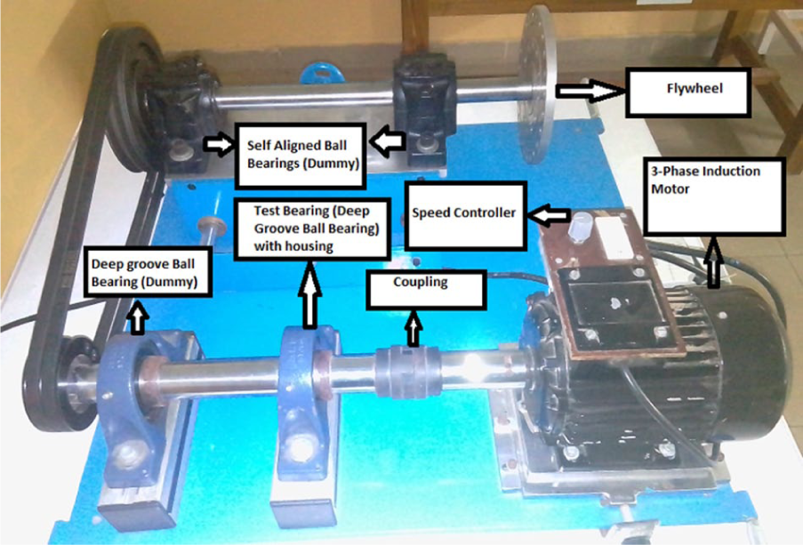
Experimental setup.

Throughout the experiment, the speed of the induction motor is kept constant at 1510 r/min. Specified and adequate lubricants are given to all the bearings before starting the experiment. The vibration readings are recorded at the sampling frequency of 2000, 1000, and 400 Hz for the frequency domain analysis and for 60-s time period in the time-domain analysis. Signals and data that are collected from the magnetic base accelerometer in the vertical direction are taken into consideration. Finally, the signal processing was done using MATLAB Wavelet design and analysis software.

Bearing geometry and characteristic frequency

The deep groove ball bearings are used in different kinds of machinery to support the load and to reduce the frictional force. Most of the problems in the machines arise due to the bearing defects. Deep groove ball bearing consists of four different elements, as, ball, inner race, outer race, and cage. During the time of operation of machine component and the bearing, the concentric localized defects may arise on the balls, inner race, outer race, and cage. These localized defects generally produce periodic impacts, whose repetition occurrence and size depend upon the revolutions per minute of the shaft, nature of the fault, and the bearing geometry. A series of impulse responses are produced by these periodic impacts. The signal spectrum consists of frequency harmonics and the resonance frequency/fault frequency is shown by the highest amplitude peaks. The load zone amplitude modulation is shown by sidebands in the amplitude–frequency plot. The bearing characteristic frequency and impulse period are the key factors to locate the defect. Hence, the bearing characteristic frequency and the period of impulse are the deciding factors to locate the bearing defects.

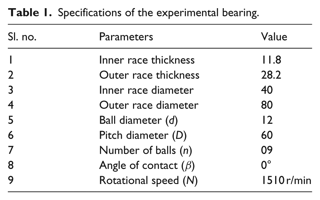
The characteristics frequencies of the bearings are calculated based on their geometry and operational speed. Each bearing has its own specified characteristic frequency for the defects. The specifications of the SKF make deep groove ball bearings (YAR 208-2F) that we have used in our research work are given in Table 1.

Table 1.

Specifications of the experimental bearing.

Sl. no.	Parameters	Value
1	Inner race thickness	11.8
2	Outer race thickness	28.2
3	Inner race diameter	40
4	Outer race diameter	80
5	Ball diameter (d)	12
6	Pitch diameter (D)	60
7	Number of balls (n)	09
8	Angle of contact (β)	0°
9	Rotational speed (N)	1510 r/min

The basic assumptions that are taken into consideration while deriving the bearing characteristic frequencies are as follows: constant angular rotation of inner and outer race, there is no slip among the bearing elements, the bearing elements are rigid in nature, and throughout the working condition, the pressure angle remains constant.

The characteristic frequencies of the test bearing are as follows²²

\begin{array}{l} Ball pass frequency of outer race (BPFO) = \\ (n / 2) \times (N / 60) [1 - (d / D) \cos β] \end{array}

(1)

\begin{array}{l} Ball pass frequency of inner race (BPFI) = \\ (n / 2) \times (N / 60) [1 + (d / D) \cos β] \end{array}

(2)

\begin{array}{l} Ball spin frequency / rolling element \\ frequency (BSF) = \\ (D / d) \times (N / 60) [1 - {(d / D)}^{2} \cos^{2} β] \end{array}

(3)

\begin{array}{l} Fundamental train frequency (FTF) / \\ cage frequency = \\ (1 / 2) \times (N / 60) [1 - (d / D) \cos β] \end{array}

(4)

Therefore, according to the above equations, the test bearing characteristic frequencies of outer race, inner race, ball, and cage are calculated to be 90.6, 135.9, 108.72, and 10.066 Hz, respectively. These characteristic frequencies are basically needed to detect the fault in ball bearings.

Modes of bearing failure and fault generation in the shaft bearing system

The faults in the ball bearing are caused by fatigue loading, wear, corrosion, electrical erosion, plastic deformation, fracture, or presence of foreign particles in the lubricant. Basically, these solid particles present in the contaminated lubricants cause damage to the ball, inner race, and outer race (Figure 2). There is a great change in the viscosity value of the contaminated lubricating oil. These foreign particles in the contaminated lubricating oil produce a scratch mark of different sizes on the bearing surface and it is the prime reason for excessive vibration.

Figure 2.

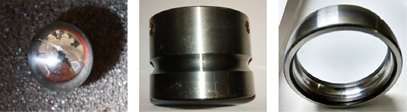
Bearing components with faults induced in the ball, inner race, and outer race.

In the test bearing, the artificial fault of dimensions of 500, 1000, and 1500 µm are cut circumferentially on the ball, inner race, and outer race. These faults are generated using electrical discharge machine (EDM) and the electrode required for the EDM to generate fault is cut using wire electrical discharge machine (wire-EDM) (Figure 3).

Figure 3.

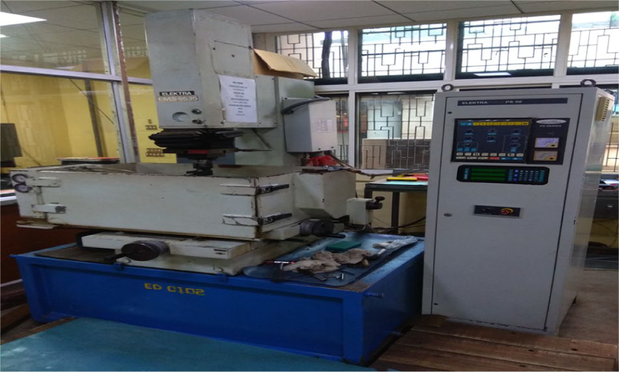
Electrical discharge machine (EDM).

It is a well-known fact that shaft misalignment in the machine component can generate vibration. The fault due to shaft misalignment has its specialized vibration signature pattern. The alignment of the total experimental setup was done using SKF laser alignment system (Figure 4). This laser alignment system has the provision to indicate both lateral and angular misalignment/offset values.

Figure 4.

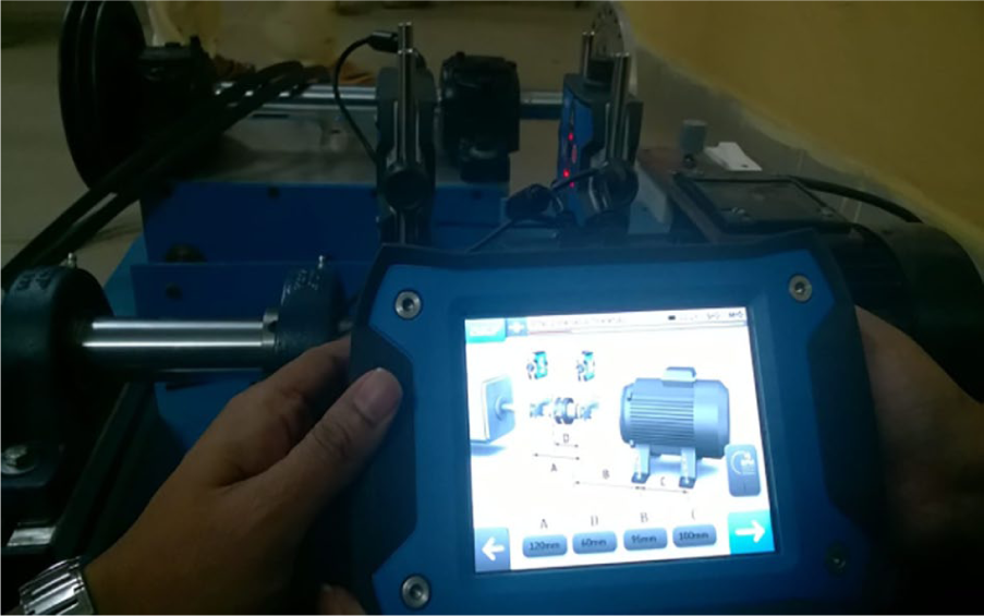
SKF laser alignment system.

The following bearing and shaft conditions are taken into account for the experimentation:

Fresh bearing.

Bearing with ball fault.

Bearing with inner race fault.

Bearing with outer race fault.

Fresh bearing with misalignment.

Fresh bearing with unbalance.

Combined faults on bearing components and shaft (ball and inner race fault, ball and outer race fault, inner race and outer race fault, ball–inner race and outer race fault, ball fault and misalignment, ball fault and unbalance, inner race fault and misalignment, inner race fault and unbalance, outer race fault and misalignment, outer race fault and unbalance).

These generated faults on the test bearing surface and the shaft can lead to the change and enhancement of amplitude and frequency of vibration. Thus, the signals from each type of fault through FFT analyzer are recorded and analyzed through the MATLAB signal processing tool to detect the severity of the fault.

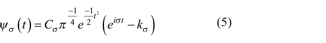
Complex Morlet wavelet

When a complex exponential (carrier) is multiplied by a Gaussian window (envelop), then it will generate a Morlet wavelet.²³ The human perception, that is, both hearing and vision, is closely related to the Morlet wavelet.

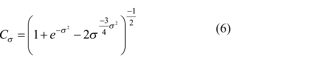
The wavelet is defined as a constant $k_{σ}$ subtracted from a plane wave and then localized by a Gaussian window

ψ_{σ} (t) = C_{σ} π^{\frac{- 1}{4}} e^{\frac{- 1}{2} t^{2}} (e^{i σ t} - k_{σ})

(5)

where $k_{σ} = e^{\frac{- 1}{2} t^{2}}$ is defined by the admissibility criterion and the normalization constant $C_{σ}$ is

C_{σ} = {(1 + e^{- σ^{2}} - 2 σ^{\frac{- 3}{4} σ^{2}})}^{\frac{- 1}{2}}

(6)

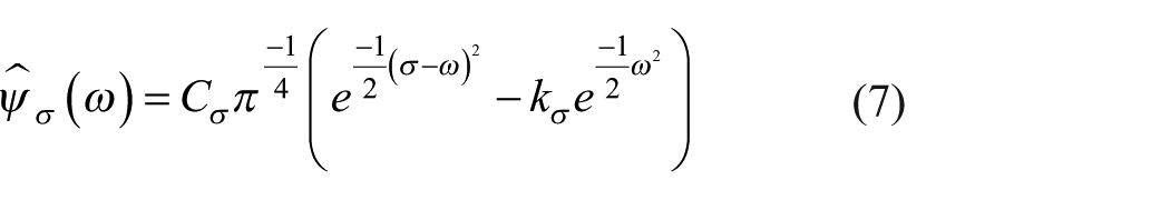
The Fourier transform of the Morlet wavelet is

{\hat{ψ}}_{σ} (ω) = C_{σ} π^{\frac{- 1}{4}} (e^{\frac{- 1}{2} {(σ - ω)}^{2}} - k_{σ} e^{\frac{- 1}{2} ω^{2}})

(7)

The “central frequency” $ω_{ψ}$ is the position of the global maximum ${\hat{ψ}}_{σ} (ω)$ which, in this case, is given by the positive solution to

ω_{ψ} = σ \frac{1}{1 - e^{- σ ω_{ψ}}}

(8)

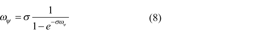
which can be resolved by a fixed-point iteration beginning at $ω_{ψ} = σ$ (the fixed-point iterations converge to the unique positive solution for any initial $ω_{ψ} > 0$ ).

The purpose of σ in the Morlet wavelet allows trade between time and frequency resolutions. Conventionally, the restriction σ > 5 is used to avoid problems with the Morlet wavelet at low σ (high temporal resolution).

Deep groove ball bearing fault detection based on the complex Morlet wavelet analysis

Fresh bearing

The original time form vibration signal of fresh bearing is shown in Figure 5. It is understandable from the figure that impacts of the periodic pattern are present in the time form vibration signal. There are no such considerable variations in the peak amplitude of the vibration signal. Figure 5 clearly indicates that there are no such considerable variations of the frequency content.

Figure 5.

Time-domain signature of fresh bearing.

Figure 6 shows the FFT of the vibration signal of the fresh bearing. The figure indicates that there is no characteristic defect frequency component and the harmonics present in the signal.

Figure 6.

Frequency-domain signature of fresh bearing.

The complex Morlet wavelet transform is applied to the data of Figure 5 to generate its amplitude and phase map. Figure 7 indicates the amplitude and phase map of the Morlet wavelet. The Morlet wavelet amplitude and phase map clearly indicate that the vibration signature does not specify any fault feature.

Figure 7.

The Morlet wavelet amplitude and phase map of vibration signal with fresh bearing.

1000 µm ball and inner race fault

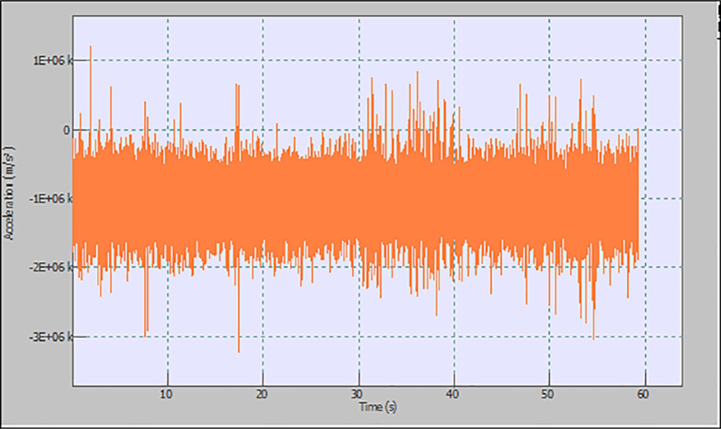
The time form vibration signal of bearing with the combined ball and inner race fault of 1000 µm is shown in Figure 8. It is understandable from the figure that impacts of the periodic pattern are present in the time form vibration signal. There are considerable variations in the peak amplitude of the signal and major variations are observed in the frequency content of the signal. Figure 8 is not sufficient to detect the characteristic period of the ball and inner race fault.

Figure 8.

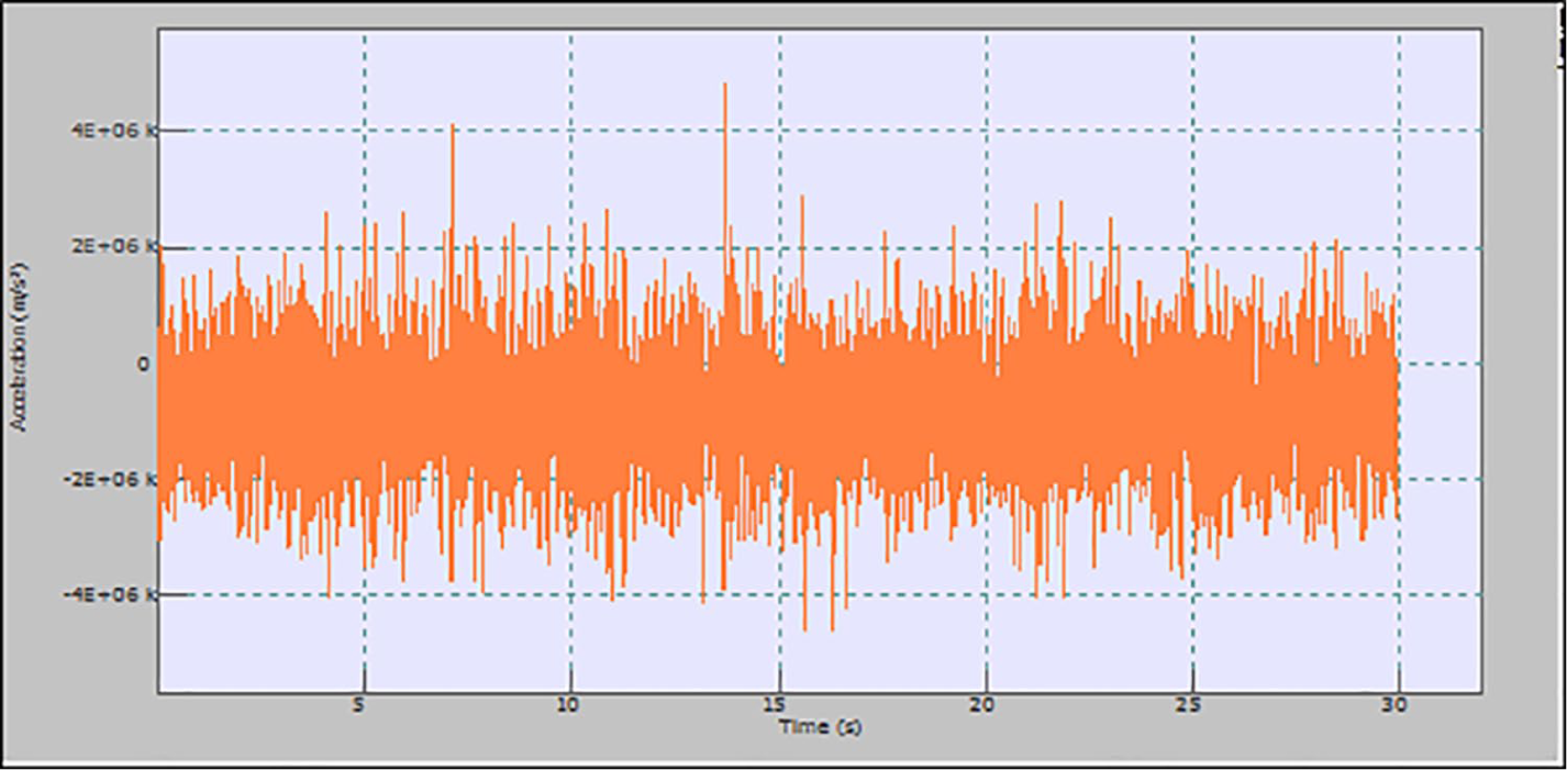
Time-domain signature of the ball and inner race fault (1000 µm) bearing.

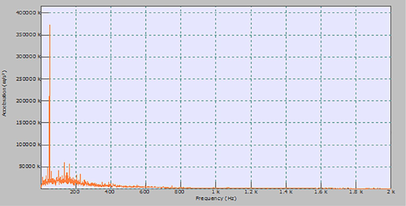
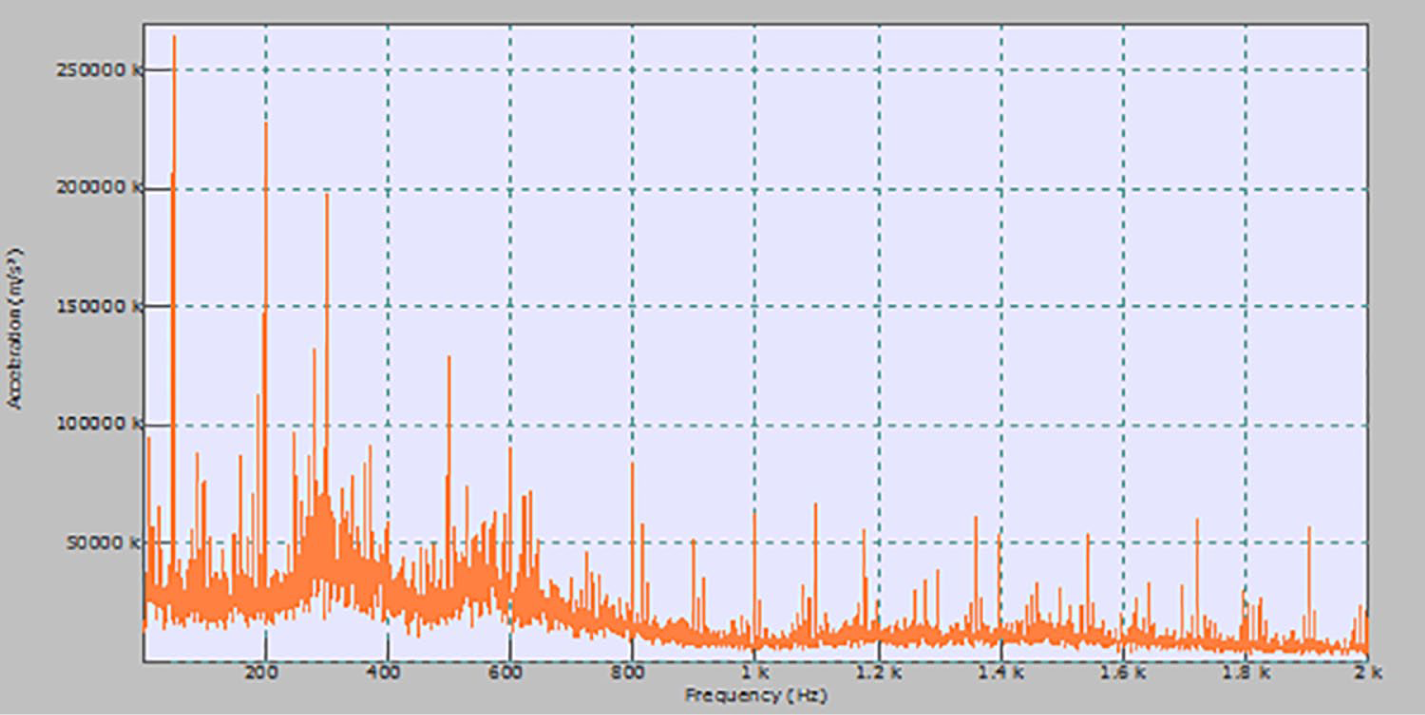
Figure 9 indicates the FFT signature of bearing having ball and inner race fault of 1000 µm. There is no such appreciable value of characteristic defect frequency components around the theoretical characteristic frequency of ball and inner race and its harmonics. Therefore, the Fourier transformation review has limitations to draw out the defect frequency of the ball and inner race signature of the bearing effectively.

Figure 9.

Frequency-domain signature of the ball and inner race fault (1000 µm) bearing.

The complex Morlet wavelet transform is applied to the data of Figure 8, which generates the corresponding amplitude and phase map. The amplitude and phase map of the Morlet wavelet are shown in Figure 10. Figure 10 clearly indicates the distinctive vibration signature with the ball and inner race fault. The sudden increase occurs in the vibration energy level due to the presence of ball and inner race fault. The characteristic defect frequency and its higher-order harmonics show the transient vibrations caused by the rolling element bearing defects. A repetitive pattern is shown by these transient vibrations, which is the indication of monotonous characteristics defect of the ball and inner race. At the resonant frequencies, a train of transient vibration is shown by the excited intrinsic mode of the rolling element bearing, which is the outcome of the ball and inner race fault.

Figure 10.

The Morlet wavelet amplitude and phase map of vibration signal with the ball and inner race fault (1000 µm) bearing.

In comparison with the amplitude map, the phase wavelet map is much clearer. A more sensitive indication is shown by the phase wavelet map than the amplitude map. An unclear pattern is shown in the phase wavelet map for scales below 33. The reason behind the unclear patter is that the signals get contaminated by the noise source for low scales.

Hence, it is concluded that the phase and amplitude map of the Morlet wavelet can be utilized as a vital signal processing tool to get rid of undesired modulation effects. The Morlet wavelet amplitude and phase map are proved to be a potential tool for the diagnosis of bearing fault (Figures 11 –13).

Figure 11.

Time-domain signature of the ball and inner race fault (1500 µm) bearing.

Figure 12.

Frequency-domain signature of the ball and inner race fault (1500 µm) bearing.

Figure 13.

The Morlet wavelet amplitude and phase map of vibration signal with the ball and inner race fault (1500 µm) bearing.

ANN

It is a subfield of artificial intelligence. ANN consists of several layers such as input, hidden, and output layer. The various neurons are present in each layer. The neurons present in the input layer represent the raw data provided to the system. The input layer is attached to the hidden layer through some weights. Finally, the hidden layer is attached to the output layer which receives the desired output, which can be represented as²⁴

Y = f (\sum_{i = 1}^{n} a_{i} w_{i} + b)

(9)

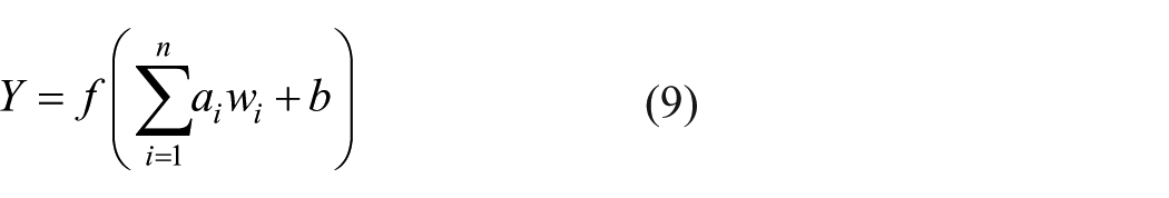
where Y is the output of the neuron, b is the bias, a_i is the input of a neuron, and w_i is the weight associated with the corresponding inputs.

The neural network can be used as a tool for prediction and classification of faults. Pattern recognition tool can be used as a classifier to classify the faults and recognize a followed pattern.

The inputs and outputs are imported in the MATLAB workspace and “nptool” is used and data are trained. Here, training algorithms used are scaled conjugate gradient (trainscg) backpropagation. The performance function is mean square error (MSE). The connection weights are modified to train the network and to optimize the performance criterion the network is biased iteratively. The network is trained repetitively and the network which produces the lowest validation error during training was selected as the optimum network. An MSE of 10⁻³, a minimum gradient of 10⁻¹⁰, and a maximum of 1000 numbers of the epoch are used and if any one of these conditions is met, then the training process would stop automatically.

A total of 4000 data are considered for training and validating the neural network. Out of which 2000 data each are corresponding to the fresh and faulty bearing of the same frequency. For training and validation purpose, 15% (for both cases) of the total data has been considered. Also, in some of the cases for a better classification, we have taken 20% of total data for training and 20% of total data for validation.

A confusion matrix is a supervised learning error matrix, which is used to check the performance of a classifier on a set of test data for which the true values are known. The performance of an algorithm is clearly visualized by the confusion matrix. There are four confusion matrices namely training confusion matrix, validation confusion matrix, test confusion matrix, and all-confusion matrix. The columns of the confusion matrix represent the target class and the rows represent output class while the diagonal cells represent the percentage of the output and target classes matches. The off-diagonal cell represents the percentage of classes mismatched. The far-right column shows the accuracy of the output class and rows at the bottom shows the accuracy of the target class, while the cell at right bottom shows the overall accuracy.²⁵

Here, in the present research, classification based on the binary scheme is implemented to represent the condition of the bearing in the pattern recognition classifier, as fresh bearing (1 0 0), inner race fault (0 1 0), and outer race fault (0 0 1) to indicate the conditions of the bearing.

500 µm outer race fault

Figure 14 shows the confusion matrix for fresh and outer race fault of 500 µm. The all-confusion matrix shows that 75% of bearing faults were classified successfully. Hence, we can say that pattern recognition tool of ANN is having a better level of accuracy in the classification of bearing faults (Figure 15).

Figure 14.

All-confusion matrix of fresh bearing and outer race fault of 500 µm.

Figure 15.

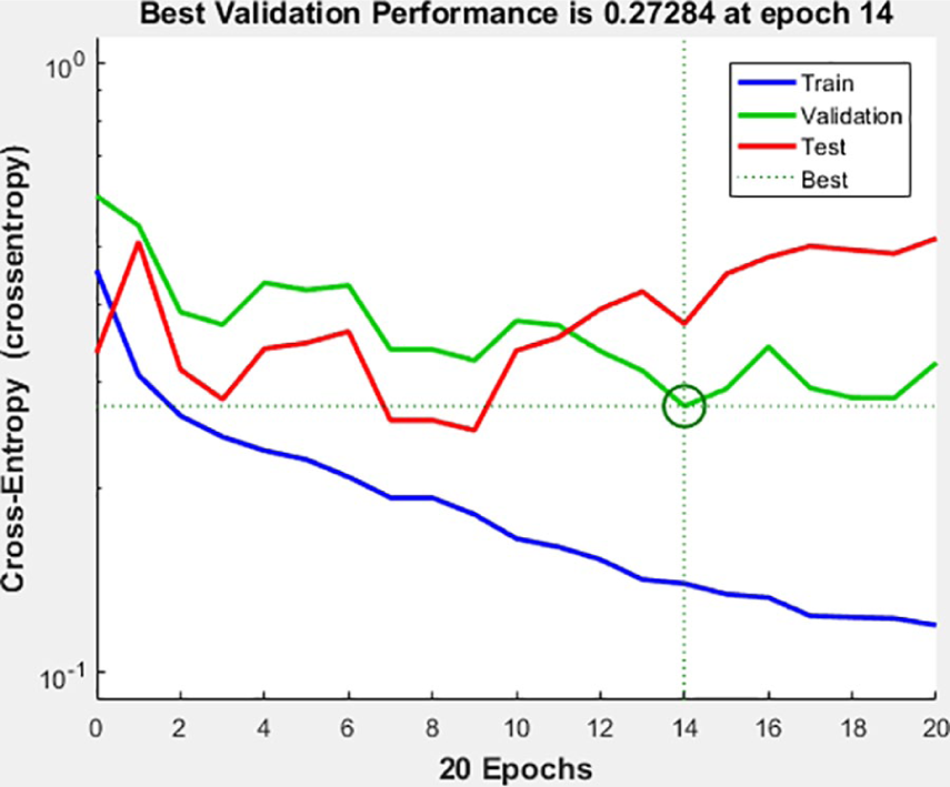
Best validation performance graph for fresh bearing and outer race fault of 500 µm.

The above graph indicates that 14 epochs are required by ANN to achieve the required target. We know that an MSE of zero value indicates no error in the training process of the ANN. On the contrary, a higher error percentage is shown during the training process of the neural network if the MSE is greater than 0.5. Hence, for a better training result, the MSE should be within an acceptable range of 0.5. In the above graphical representation, MSE is 0.27284, which is within an acceptable range. It represents that the ANN implemented for the bearing fault diagnosis was correct and being used successfully for the allotted task.

1000 µm ball and inner race fault

Figure 16 shows the confusion matrix for fresh and ball–inner race fault of 1000 µm. The all-confusion matrix shows that 98.4% of bearing faults were classified successfully. Hence, we can say that pattern recognition tool of ANN is having a better level of accuracy in the classification of bearing faults (Figure 17).

Figure 16.

All-confusion matrix of fresh bearing and ball–inner race fault of 1000 µm.

Figure 17.

Best validation performance graph for fresh bearing and ball–inner race fault of 1000 µm.

The above graph indicates that 101 epochs are required by ANN to achieve the required target (Table 2). We know that an MSE of zero value indicates no error in the training process of the ANN. On the contrary, a higher error percentage is shown during the training process of the neural network if the MSE is greater than 0.5. Hence, for a better training result, the MSE should be within an acceptable range of 0.5. In the above graphical representation, MSE is 0.084224, which is within an acceptable range. It represents that the ANN implemented for the bearing fault diagnosis was correct and being used successfully for the allotted task.

Table 2.

ANN accuracy percentage and best validation performance for different fault types.

Sl. no.	Fault type	ANN input combination	Accuracy (of all-confusion matrix)	Best validation performance
1	500 µm single fault	Fresh bearing and ball fault	72.9% (70-15-15)	0.10487 at epoch 18
		Fresh bearing and inner race fault	75% (80-10-10)	0.14062 at epoch 19
		Fresh bearing and outer race fault	75% (80-10-10)	0.27284 at epoch 14
2	1000 µm single fault	Fresh bearing and inner race fault	90.4% (70-15-15)	0.22935 at epoch 132
		Fresh bearing and outer race fault	88.9% (80-10-10)	0.31702 at epoch 108
		Fresh bearing and ball fault	93.8% (60-20-20)	0.19371 at epoch 108
3	1000 µm combination fault	Fresh bearing and inner + outer race fault	98.6% (60-20-20)	0.054921 at epoch 73
		Fresh bearing and ball + inner race fault	98.4% (70-15-15)	0.084224 at epoch 101
		Fresh bearing and ball + outer race fault	100% (70-15-15)	4.9204e-06 at epoch 59
4	Misalignment and unbalance	Fresh bearing and misalignment	95.7% (70-15-15)	0.21735 at epoch 42
Fresh bearing and unbalance	70.5% (70-15-15)	0.63962 at epoch 54

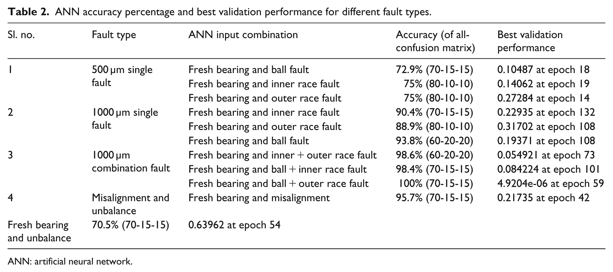
ANN: artificial neural network.

Classification learner

Classification learner is a supervised machine learning application (Figure 18). Classification learner helps to classify data by training the required data which needs to be classified; also predictions can be made with best-trained models by exporting it to the workspace and providing the new data of same data type as trained data.

Figure 18.

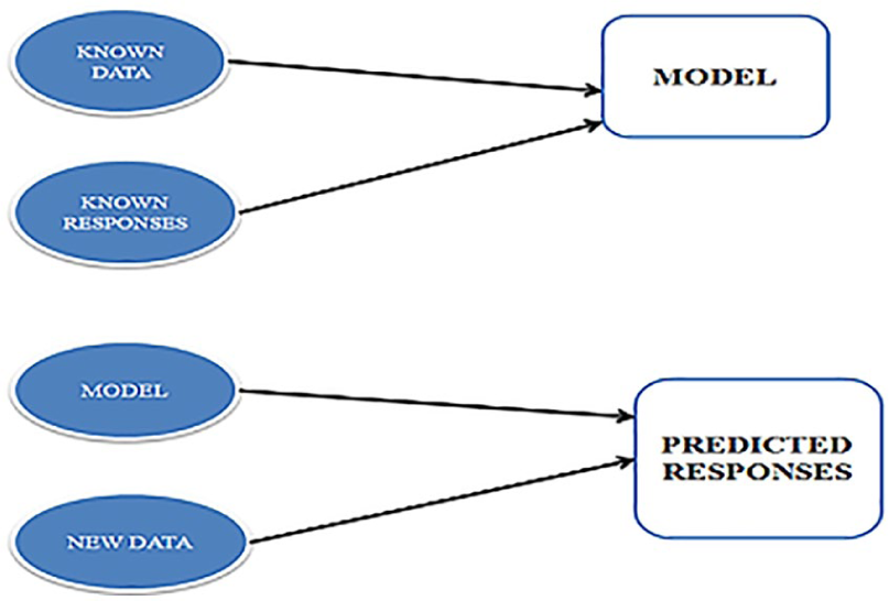
Use of classification learner to obtain model and predicted response.

The methods of classifying a data or classification learner are as follows: The classification methods are also known as classification models, so they are listed in the following:

Decision trees,

Discriminant analysis,

Logistic regression classifier,

SVMs,

Nearest neighbor classifier,

Ensemble classifier.

SVMs

SVMs have been opted for training data which have two or more classes. After training the data, it is required to generate C coding for the prediction of the results. In SVMs, binary or multi-class classification methods have been opted for the data type. SVMs have low to high prediction speed, easy to hard interpretability, and low to large memory usage. Also, it has low to high flexibility depending upon the data type.

The SVMs classify data by searching for the best hyper-plane which distinguishes data points between two classes. The largest margin between the two classes shows the best hyper-plane for the SVMs. Margin is the maximal width of the slab which is parallel to the hyper-plane and has no data points in the interior.

On the boundary of the slab, the data points which are closest to the hyper-plane separating the data points are known as support vectors.

Figure 19 shows data points of type +1 and data points of type ‒1. The equation of hyper-plane is given as

W . X + b = 0

(10)

Here, W and b are the linear classifiers which are used to separate the classes; and X is a point on a hyper-plane.

Figure 19.

SVMs hyper-plane separating the data points by a margin.

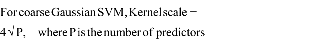
SVM is a supervised learning method of machine learning. Different SVM techniques have been implemented in this research work to classify the bearing data. Here velocity and acceleration values are used as input parameters to indicate fresh and faulty bearings. In the SVM datasheet, bearing type “FRESH” or “FAULT” is being used to indicate fresh and faulty bearings, respectively. The fivefold cross-validation method was selected to classify the data. The fivefold cross-validation protects the data from over-fitting and calculates the accuracy by dividing the data into multi-folds and then going for the calculation of the accuracy of each fold. The training of the model was done by implementing different SVM techniques, such as linear SVM, quadratic SVM, cubic SVM, fine Gaussian SVM, medium Gaussian SVM, and coarse Gaussian SVM. The kernel scale and kernel function were selected manually to achieve a greater level of accuracy. Generally, the kernel scale for different kernel functions is calculated using the following equation

\begin{array}{l} For fine Gaussian SVM, Kernel scale = \\ \sqrt P \div 4, where P is the number of predictors \end{array}

\begin{array}{l} For medium Gaussian SVM, Kernel scale = \\ \sqrt P, where P is the number of predictors \end{array}

\begin{array}{l} For coarse Gaussian SVM, Kernel scale = \\ 4 \sqrt P, where P is the number of predictors \end{array}

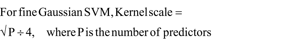
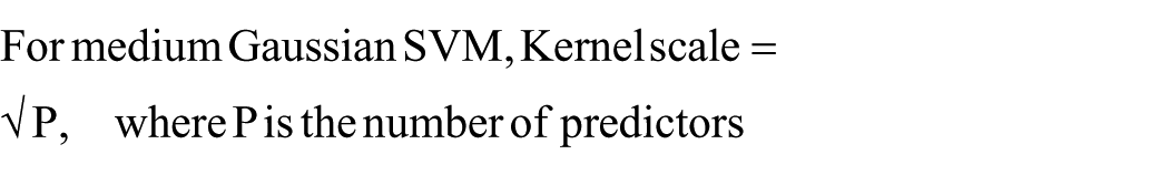
To reduce the dimensionality, the principal components analysis (PCA) was kept off. The model prediction and class separation were investigated by scatter plot. The confusion matrix was plotted to check the performance of the classifier.

The receiver operating characteristic (ROC) curve was plotted to check the positive rate/negative rate of the trained model. The area under the curve (AUC) was used to check the overall performance of the classifier. Larger the AUC number, better the classifier performance.

We can predict new data by exporting the best-trained model to the workspace. But the work in this article is only related to the classification of the data. Therefore, the accuracy of the classification is the prime concern for this research work (Table 3).

Table 3.

SVM (fine Gaussian) accuracy percentage for different fault types.

Sl. no.	Fault type	SVM input combination	Accuracy (%)
1	500 µm	Fresh bearing + ball fault	90.30
		Fresh + ball + inner + outer race fault	91.40
		Outer race fault	88.50
		Inner race fault	97.60
2	1000 µm	Ball fault	97.70
		Inner + outer race fault	99.40
		Inner race fault	96.50
		Outer race fault	95.50
		Ball + inner race fault	99.20
		Ball + outer race fault	98.90
3	1500 µm	Ball fault + unbalance (high)	98.20
		Ball fault + inner race fault	97.80
		Ball fault + outer race fault	99.20
		Ball fault	97.10
		Inner race + outer race fault	99.50
		Inner race + misalignment (high)	92.50
		Inner race fault	97.50
		Inner race + unbalance (high)	90.20
		Outer race + misalignment (high)	98.10
		Outer race + unbalance (high)	99.70
		Outer race fault	99.00
4	Unbalance	Fresh bearing with unbalance (high)	91.70
		Fresh bearing + unbalance (medium)	86.80
		Fresh bearing + unbalance (low)	83.30
5	Misalignment	Fresh bearing with misalignment (low)	98.40
		Fresh bearing with misalignment (high)	98.90
		Fresh bearing with misalignment (medium)	86.40
6	Combination	1500 µm ball fault and 500 µm inner race fault	98.30

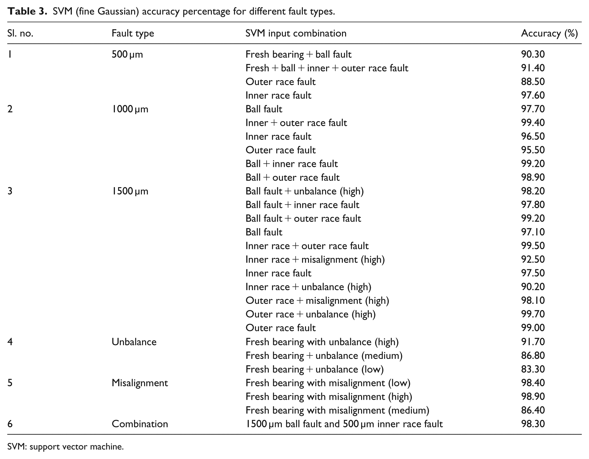
SVM: support vector machine.

500 µm inner race fault

SVM scatter plot and SVM ROC curve of fresh bearing and inner race fault of 500 µm are shown in Figures 20 and 21.

Figure 20.

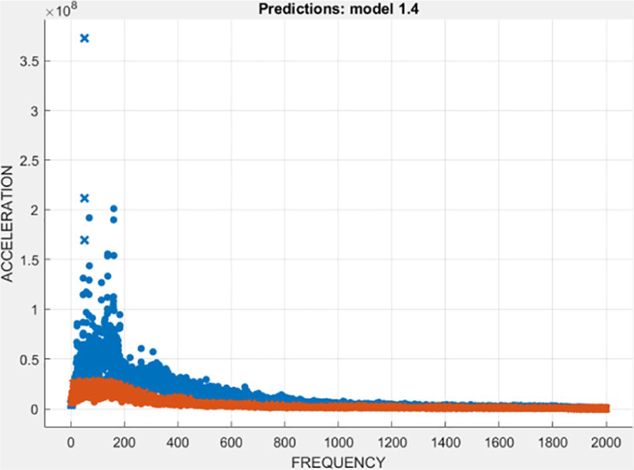
SVM scatter plot of fresh bearing and inner race fault of 500 µm.

Figure 21.

SVM ROC curve of fresh bearing and inner race fault of 500 µm.

1000 µm inner and outer race fault

SVM scatter plot and SVM ROC curve of fresh bearing and inner–outer race fault of 1000 µm are shown in Figures 22 and 23.

Figure 22.

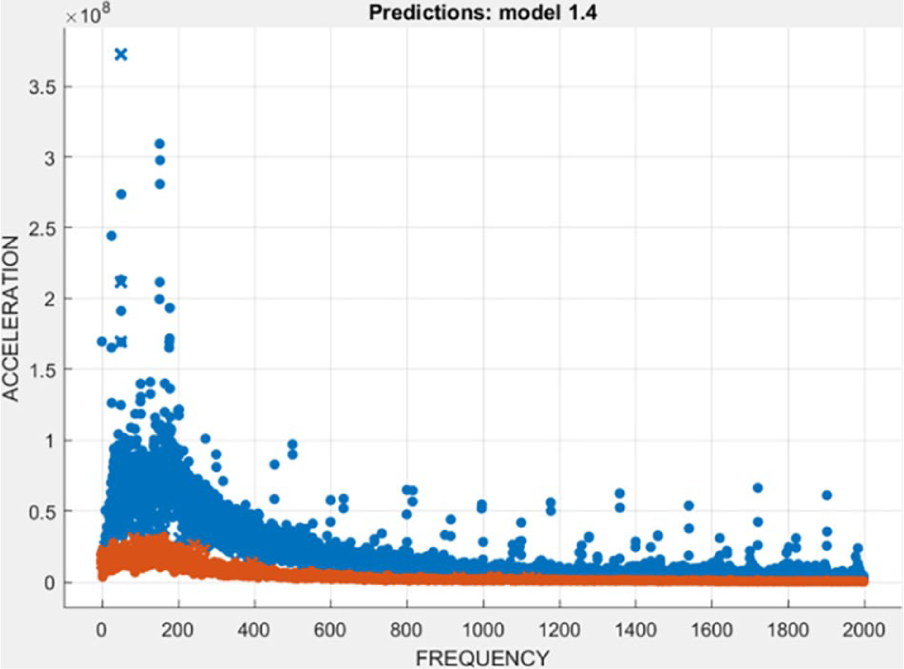
SVM scatter plot of fresh bearing and inner–outer race fault of 1000 µm.

Figure 23.

SVM ROC curve of fresh bearing and inner–outer race fault of 1000 µm.

1500 µm outer race fault and unbalance (high)

SVM scatter plot and SVM ROC curve of fresh bearing and outer race fault–unbalance of 1500 µm are shown in Figures 24 and 25.

Figure 24.

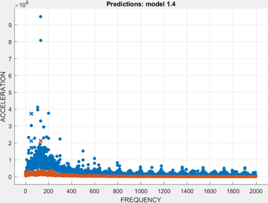
SVM scatter plot of fresh bearing and outer race fault–unbalance of 1500 µm (high).

Figure 25.

SVM ROC curve of fresh bearing and outer race fault–unbalance of 1500 µm (high).

For this research, the classification accuracy shows that SVM is a better classifier than ANN. The performance of SVM is observed to be superior due to its better generalization capability. The mean accuracy level of SVM is found to be 95.271%, which is more than the accuracy level of ANN, that is, 87.2%.

Conclusion

This article proposed a method to detect the single and combined faults of the rolling element bearing. The complex Morlet wavelet analysis is selected as an extraction tool to detect the fault feature and characteristics of the vibration signal of rolling element bearing. This research work clearly indicated that the complex Morlet phase and amplitude plots are potential tools in the identification and diagnosis of rolling element bearing faults. The amplitude and phase map of the complex Morlet wavelet are found to show unique informative signatures in the presence of bearing faults. The complex Morlet wavelet enables extraction of the transient, which is the indicator of a defect in the rolling element bearing signature. Hence, it becomes possible to detect the fault features and the information regarding the nature of fault from the vibration signal.

This research work implements two artificial intelligence techniques, namely ANN and SVM, for detection and classification of bearing faults. The results of fault classification with SVM are superior to ANN. These results show the practical application of the complex Morlet wavelet and artificial intelligence techniques for early fault detection and classification in the rolling element bearings. Therefore, effective maintenance strategies can be implemented to prevent sudden failure and to reduce maintenance costs.

Footnotes

Declaration of conflicting interests

The author(s) declared no potential conflicts of interest with respect to the research, authorship, and/or publication of this article.

Funding

The author(s) received no financial support for the research, authorship, and/or publication of this article.

ORCID iD

Chandrabhanu Malla

References

Kankar

Sharma

Harsha

SP.

Rolling element bearing fault diagnosis using wavelet transform. Neurocomputing 2011; 74: 1638–1645.

Ali

Fnaiech

Saidi

, et al. Application of empirical mode decomposition and artificial neural network for automatic bearing fault diagnosis based on vibration signals. Appl Acoust 2015; 89: 16–27.

Wang

Enhancement of signal denoising and multiple fault signatures detecting in rotating machinery using dual-tree complex wavelet transform. Mech Syst Signal Pr 2010; 24: 119–137.

Bearing fault detection based on order tracking and Complex Morlet wavelet transform. Key Eng Mat 2011; 474–476: 639–644.

Kumar

Pai

Sriram

, et al. ANN based evaluation of performance of wavelet transform for condition monitoring of rolling element bearing. Procedia Engineer 2013; 64: 805–814.

Yang

Liu

, et al. Compound faults detection of the rolling element bearing based on the optimal Complex Morlet wavelet filter. Proc IMechE, Part C: J Mechanical Engineering Science 2018; 232: 1786–1801.

Tyagi

Panigrahi

SK.

A DWT and SVM based method for rolling element bearing fault diagnosis and its comparison with Artificial Neural Networks. J Appl Comput Mech 2017; 3(1): 80–91.

Zheng

Bearing fault diagnosis based on amplitude and phase map of Hermitian wavelet transform. J Mech Sci Technol 2011; 25(11): 2731–2740.

Nikolaou

Antoniadis

IA.

Demodulation of vibration signals generated by defects in rolling element bearings using complex shifted Morlet wavelets. Mech Syst Signal Pr 2002; 16(4): 677–694.

10.

Rubini

Meneghetti

Application of the envelope and wavelet transform analysis for the diagnosis of incipient faults in ball bearings. Mech Syst Signal Pr 2001; 15(2): 287–302.

11.

Junsheng

A roller bearing fault diagnosis method based on EMD energy entropy and ANN. J Sound Vib 2006; 294(1): 269–277.

12.

, et al. Bearing fault diagnosis based on multi scale permutation entropy and support vector machine. Entropy 2012; 14(8): 1343–1356.

13.

Barkov

Barkova

Mitchell

JS.

Condition assessment and life prediction of rolling element bearings. Sound Vib 1995; 10(17): 27–31.

14.

Samantha

Al-Balushi

KR.

Artificial neural networks based fault diagnostics of rolling element bearings using time domain features. Mech Syst Signal Pr 2003; 17: 317–328.

15.

Tondon

Choudhury

An analytical model for the prediction of the vibration response of rolling element bearings due to a localized defect. J Sound Vib 1997; 205(3): 275–292.

16.

Paya

Esat

Badi

MNM

. Artificial neural networks based fault diagnostics of rotating machinery using wavelet transforms as a preprocessor. Mech Syst Signal Pr 1997; 11: 751–765.

17.

Prabhakar

Mohanty

Sekhar

AS.

Application of discrete wavelet transform for detection of ball bearing race fault. Tribol Int 2002; 3(12): 793–800.

18.

Rafiee

Tse

Harifi

, et al. A novel technique for selecting mother wavelet function using an intelligent fault diagnosis system. Expert Syst Appl 2009; 36: 4862–4875.

19.

Kankar

Sharma

Harsha

SP.

Fault diagnosis of ball bearings using machine learning methods. Expert Syst Appl 2011; 38: 1876–1886.

20.

Jardine

Lin

Banjevic

A review on machinery diagnostics and prognostics implementing condition based maintenance. Mech Syst Signal Pr 2006; 20(7): 1483–1510.

21.

Feng

Jiang

Rolling element bearing fault detection based on optimal antisymmetric real Laplace wavelet. Measurement 2011; 44: 1582–1591.

22.

Malla

Panigrahi

Review of condition monitoring of rolling element bearing using vibration analysis and other techniques. J Vib Eng Technol 2019; 7(4): 407–414.

23.

Toth

On finding better wavelet basis for bearing fault detection. Acta Polytechn Hung 2013; 10(3): 17–35.

24.

Dubey

Agrawal

Bearing fault classification using ANN-based Hilbert footprint analysis. IET Sci Meas Technol 2015; 9(8): 1016–1022.

25.

Bhavaraju

Kankar

Sharma

, et al. A comparative study on bearing faults classification by artificial neural networks and self-organizing maps using wavelets. Int J Eng Sci Tech 2010; 2(5): 1001–1008.