Traffic noise models and noise guidelines: A review

Abstract

Traffic noise is a major cause of noise pollution, and impacts of noise pollution on humans have been studied extensively. Previous studies have helped in the development of traffic noise prediction analysis using robust analytical and computational models, parameters connected with traffic, road characteristics, and environment. This study reviewed 11 traffic noise modeling strategies and parameters used by various agencies in different parts of the world. Seven out of the 11 models reviewed in this paper were based on outdoor measurements while the remaining four were based on outdoor and indoor measurements. Considering the cost and time involved in developing these models, there is need to understand existing traffic noise models, differences, and assumptions before adopting or recalibrating them for local demands. This study contributes to the larger body of knowledge and intends to serve as a reference material for future researchers in the area of traffic noise modeling and techniques.

Keywords

Traffic noise emission models noise guidelines

Introduction

Roadways are vital to a region’s socio-economic growth as they serve as the primary mode of transport. Transport systems sustain trade both at national and global levels, as well as provide accessibility to the basic needs of life. However, transport operations have several detrimental effects on the ecosystem and the public.¹ They are, but not limited to, the following: air and noise pollution; exposure to these have been studied by researchers to have a series of demonstrable health consequences, both physical and emotional. In recent years, several studies have identified traffic noise as one of the leading environmental problems globally. The problem is more pronounced in built-up areas. The traffic noise menace is generally associated with urban sprawl, progress in technology, and the extension of roadway infrastructure, triggering environmental nuisances. This situation often tends to increase, particularly in rapidly urbanizing cities, where motorization is also on the increase. In response to these social problems and significant health concerns regarding ambient noise, the European Union (EU) carried out the Directive 2002/49/EC. The goal of the EU is to ensure that environmental exposure to most traffic and industrial noise is avoided or reduced.

Previous research as in Ref. [2,3] divided the effect of traffic noise into four subcategories based on intensity and duration: physical effects (hearing defects), psychological effects (irritability, sleeplessness, and stress), physiological effects (hypertension and abnormal heart rhythm), and effects on work efficiency (decrease in productivity as well as misunderstanding of what is being heard). Additionally, continuous exposure to traffic noise by an individual within proximity to the roadway may lead to long-term health deterioration, like adiposity during pregnancy and risk of overweight in 7-year-old children.^4,5 Thus, urban planners and acoustic engineers have come up with strategies to curb traffic noise pollution to ensure an adequate level of service to road users and roadway sustainability.

Traffic noise monitoring data can be used to predict the level of sound intensity using various prediction models, with the aid of noise descriptors for computation and evaluation. However, the tools, technical know-how, and numerical methods of these models are quite complex and cumbersome to adopt by urban planners and, as such, there is a need for some future-oriented research perspectives on traffic noise monitoring and evaluation. This review examines factors that contribute to an increase in traffic noise levels and noise indicators measured or calculated to evaluate the impacts of traffic noise pollution. Also, by comparing models and noise guidelines developed from previous research in developed and developing cities based on their underlying traffic conditions and distinguishing their key assumptions as well as their peculiarities.

Highway noise descriptors

Noise from various sources can be determined or explained differently. An identical type of noise source is calculated or defined by alternative approaches. Scientists have carried out assessments and experimental research to establish descriptors (indicators) to better describe the range of environmental noise sources. These noise indicators represent a physical scale for the description of environmental noise, which has a relationship with an effect on human health. Some descriptors for road noise include the following:

Equivalent continuous sound level, Leq

Noise intensity changes with time; therefore, the equivalent sound level (L_eq) is described as a stable situation; it is the average rate of energy the human ear receives over the preceding duration. Hourly sound level equivalent, or L_eq(h), is frequently used by state road agencies as a traffic noise descriptor when the duration of the measurement is 1 hour.⁶

The n-percent exceeded level, L_n

Researchers focus on a time-dependent noise source when measuring traffic noise. Sounds and noise are relatively not consistent in most cases. Besides the difference in frequency, the ambient noise level varies over time. Ln is the n^th-percent of the sound pressure level exceeded over time.⁷ The frequently used values of n for the n-percent exceeded level are 10, 50, and 90.

L₁₀ is the level exceeded 10% of the time. In other words, for 10% of the time, the sound or noise has a sound pressure level above L₁₀. For the rest of the time, the sound or noise has a sound pressure level at or below L₁₀. These higher sound pressure stress levels may be due to erratic or recurring events. L₅₀ is the level exceeded 50% of the time. It is statistically the midpoint of the noise readings. It represents the median of fluctuating noise levels. L₉₀ is the level exceeded 90% of the time. It is generally considered to represent the background or ambient level of a noise environment. For a varying sound, L₁₀ is greater than L_50, which in turn is greater than L₉₀.⁷

Noise pollution level

The noise pollution level considers sound signal changes and therefore acts as a better environmental pollution indicator for community noise dissatisfaction and annoyance. Noise pollution level (NPL)⁸ expressed in dB is as

\begin{matrix} N P L = L_{e q} + a (L_{10} - L_{90}) \end{matrix}

(1)

where a = 1.0 (constant in the equation).

Traffic noise index (TNI)

A further parameter showing the level of traffic flow variance is the traffic noise index (TNI).^9,10 This is expressed as

\begin{matrix} T N I = 4 (L_{10} - L_{90}) + L_{90} - 30 \end{matrix}

(2)

Noise climate (NC)

Noise climate (NC) is the time at which sound rates increase or decrease,¹¹ and it is expressed mathematically as

\begin{matrix} N C = (L_{10} - L_{90}) \end{matrix}

(3)

where L₉₀ is above 90% of the record time, often regarded as the background noise, that is, without the presence of vehicular traffic.

Day, evening, and night equivalent noise level (L_den)

L_den is an indicator that is a composite of long-term L_eq values for day, evening, and night.

A-weighted decibels dB(A)

A low- and high-pitched sound cannot inherently be distinguished by the human ear. Statistical modifications are made to detect how a common individual hears these sounds. The adjusted measurements are known as A-weighted decibels, dB(A).

Factors contributing to traffic noise

Certain variables related to noise generation and propagation, such as traffic volume, vehicle composition, velocity, road features, etc., could have a major influence on noise prediction from vehicular traffic. Generally, these factors can be categorized into four clusters:

Traffic factors

These consist of traffic volume, traffic speed, vehicle composition, creation of traffic jams, and bottlenecks. With an increase in traffic volume, the noise level increases. A small reduction in vehicular traffic may minimize noise by reducing the average number of traffic acoustics. Trucks and buses contribute more noise to the environment compared to cars. An increase in truck traffic mix ratio will increase the noise level. For both congestion and pollution levels, the traffic mix is a significant factor. Heavy vehicles and bikes are excessively loud. Just one heavy vehicle at a speed of 30 km/h can generate noise equivalent to noise from 15 cars.¹² Traffic noise is influenced by a mixture of rolling noise (arising from the tires communicating with the roadway) and propulsion noise (such as exhaust emissions, diesel engines, motors, and brakes). Tire–road impacts are usually the main cause of sound above 55 km/h in most cars and over 70 km/h in trucks with engine sound predominating at lower speeds, although adjustments in innovation mean that rolling noise can now be controlled at rates over 20–40 km/h for brand-new vehicles and 30–60 km/h for brand-new lorries.¹³

Road factors

The state of roads is one of the key reasons for rising traffic noise pollution. Narrow roads, pavement surfaces, and recurring road maintenance all contribute to traffic jams in traffic and thus to increasing noise. These sound features are typically reliant upon appearance (smoother tires and pavement typically result in lower noise levels).¹⁴

A line of moving vehicles closely separated produces road traffic noise. This allows a recipient to experience a sequential source of noise rather than just one recognizable noise point. The noise is diminished or decreases as the distance from the highway increases. With a flat topography, each time the distance is doubled, the noise level is usually decreased by approximately 3 dB(A) as the noise level moves over rigid surfaces and approximately 4.5 dB(A) over soft surfaces when all other factors remain constant.¹⁵

Vehicle factors

Some components from the vehicle can also be a contributing factor in increasing noise, such as the noise characteristics of engine type and size, type of horn, and age of the vehicle. Vehicles exceeding 12 tons in weight and powered by engines of over 200 HP generate noise ranging from 91 to 92 dBA at a distance of 8 m, while vehicles not exceeding the weight of 3.5 tons and powered by engines not exceeding 200 HP generate noise of 85 dB(A) at the same distance from the road.¹⁶

Human factors

Reckless driving, or the driver’s frame of mind, can influence his driving and this can also be a contributing factor in noise generation. Knowledge of noise levels on the roads is required to develop and plan remedial action. Several models of traffic noise prediction have been developed and are used as a policy tool for noise prediction and highway simulation.

Traffic noise models

The fact that road noise is a pollutant has led to the development of statistical and predictive models that take into account the source, propagation, and effects on the receptor. Models for traffic noise estimation commenced over 60 years ago, and the outcomes are still reliable. In 1952, the first traffic noise model was developed as stated in the Noise Acoustics Handbook by Anon¹⁷

\begin{matrix} L_{50} = 68 + 8.5 l o g V - 20 l o g d \end{matrix}

(4)

This model considers the 50th percentile noise indicator and the input parameters are traffic volume (V) and distance (d),¹⁸ formulated a model by applying noise sources from different engine vehicles. For every engine type, its noise level varies with the engine capacity and speed

\begin{matrix} L_{A} = 30 l o g N + 17.5 l o g C \end{matrix}

(5)

\begin{matrix} L_{A} = 50 l o g N + 17.5 l o g C \end{matrix}

(6)

From equations (5) and (6), $N$ is the speed and $C$ is the engine capacity for diesel and spark-ignition engines. They concluded that the source of car noise depends mainly on operating speed. Consequently, some sound absorption recommendations rely on the car engine designer and vehicle model with a focus on limiting the maximum engine speed and thermodynamic efficiency.

Adhering to the International Standard Organization (ISO R 362),¹⁹ the authors measured these parameters to be considered for the generation of traffic noise models, which are the speed of vehicles and the height of measurement from ground level. They noted that perception from the noise source to receiver differs. Thus, the authors formulated certain noise indices which are L_m, the maximum noise level; L_eq, the equivalent noise level measured for 10 seconds; and lw, acoustic power. Therefore, the relations between them for a distance d = 7.5 m at a height of 1.2 m and different speeds (30 km/hr, 60 km/h, and 120 km/hr) of vehicles are given by

\begin{matrix} L_{e q 10} = L_{w} - 10 \log (d v) - 13 \end{matrix}

(7)

\begin{matrix} L_{e q 10} = L_{m} - 10 \log (d / v) - 5 \end{matrix}

(8)

In addition, given that several models have been built globally, the characteristics of various countries have been taken into consideration in terms of roadways, vehicles, and weather features. Several countries have adopted monitoring and controlling the use of these models, which can be implemented in the simulation of traffic noise.

FHWA model

The Federal highway administration (FHWA) model, just like several other prediction models, was developed for the United States of America as in Ref. [20]. They arrived at an estimated level of noise over several modifications. The energy emission standard for traffic streams for varying distances from the lane, for a finite length of roads, and shielding is a benchmark in the FHWA model. The following equation ties all these variables

\begin{matrix} L_{e q} (h) = L_{0 E} + 10 l o g (\frac{N π D_{0}}{S_{} T}) + 10 l o g {(\frac{D_{0}}{D})}^{1 + α} + 10 \log (\frac{(φ_{α} θ_{1}, θ_{2})}{π}) + Δ_{s} - 25 \end{matrix}

(9)

where

L_{e q} (h)

is the hourly equivalent sound level,

L_{0 E}

is the reference energy mean emission level,

N

is the number of vehicles passing a specified point during the period of 1 h,

D

is the perpendicular distance, in meters, from the centerline of the traffic lane to the observer,

D_{0}

is the reference distance (15 m) at which the emission levels are measured,

S_{}

is the average speed of vehicles in km/h, T is the period over which the equivalent sound level is computed (1 hour),

α

is a site parameter whose values depend upon site conditions,

φ

is a symbol representing a function used for segment adjustments, and

Δ_{s}

is the attenuation, in dB, provided by some type of shielding such as barriers, rows of houses, densely wooded areas, etc.

In the FHWA model, the microphone is located along the line to the middle of the lane at a 15-meter distance from the middle of the lane at a height of 1.5 m. The ground between the pavement and the microphone will be smooth and without reflective surfaces while the vehicles travel on a straight, low-speed, flat road.

When D is less than 15m, the sound level is computed as follows

\begin{matrix} L_{e q} {(h)}_{i} = L_{0 E i} + 10 \log (\frac{N_{i} D_{0}}{S_{i}}) + \frac{10 \log 1}{1 + α} {{(\frac{D_{0}}{R_{n}})}^{1 + α} - {(\frac{D_{0}}{R_{f}})}^{1 + α}} - 30 \end{matrix}

(10)

For hard site (absorptive) ground $α$ is zero, then equation (10) reduces to

\begin{matrix} L_{e q} {(h)}_{i} = L_{0 E i} + 10 l o g (\frac{N_{i} D_{0}}{S_{i}}) + 10 l o g {(\frac{D_{0}}{R_{n}}) - (\frac{D_{0}}{R_{f}})} - 30 \end{matrix}

(11)

where

R_{n}

is the distance in meters between the centerline of the near end of the roadway segment and the observer.

R_{f}

is the distance in meters between the centerline of the far end of the roadway segment and the observer. When D is less than 15 m and α is 1/2 for (soft site) a reflective site, the sound level in this situation is computed as follows

\begin{matrix} L_{e q} {(h)}_{i} = L_{0 E i} + 10 l o g (\frac{N_{i} D_{0}}{S_{i}}) + 10 l o g \frac{2}{3} {{(\frac{D_{0}}{R_{n}})}^{3 / 2} - {(\frac{D_{0}}{R_{f}})}^{3 / 2}} - 30 \end{matrix}

(12)

The technique applies only to flat roads and constant velocity cars, but approaches are used to model for curved roads and several lanes. In this model, it is assumed that emission levels within groups of all classes of vehicles are normally distributed and the loss of propagation is sufficiently reflected by distance impacts.

Interrupted flow (stop-and-go traffic) model

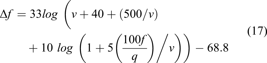
Most traffic noise models derived have been mainly based on freely moving vehicles and are consequently not applicable to traditional city roads which are disrupted by flows, such as signals, speed humps, etc., as these interrupt traffic. An equation for the estimation of disrupted flow from curbside noise was examined in this analysis. The provisional model equation was generated at College Imperial London.²¹ The equation was of the form

\begin{matrix} L_{10} = 55.7 + 9.18 l o g Q (1 + 0.09 H) - 4.20 l o g V_{y} + 2.13 T \end{matrix}

(13)

where

Q

is the traffic volume,

H

is the proportion of heavy vehicles,

T

is the index of dispersion,

V

is the mean speed of traffic (km/h), and

y

is the carriageway width. The conceptual equation estimates curbside noise levels which can be used in roads with a traffic lane width of 6–15 m and speeds are in the range of 20–50 km/h. Several validation tests were carried out, and the following formula was obtained

\begin{matrix} L_{10} = 48.50 + 10.52 l o g 10 Q (1 + 0.04 H) - 5.74 l o q 10 (d k + 0.5 y) + 2.38 l o g 10 G \end{matrix}

(14)

where

d k

is the distance to the curb from the measurement and

G

is the gradient = 1.

This equation did not provide the dispersion factor, $T$ , which is the ratio of variance to the mean of traffic volume or the average speed, and would, therefore, be simpler to use than the tentative equation.

CoRTN model

The Calculation of Road Traffic Noise Model²² (CoRTN) procedure for the estimation of road traffic noise was developed for the United Kingdom by the Department of Transport. This model postulates a line source of noise traffic and steady speed traffic and is the only method in Britain for evaluating the potential impacts of vehicular traffic by highway agencies.¹⁷

The CoRTN traffic noise prediction model is

\begin{matrix} L_{10} = L_{0} + Δ f + Δ p + Δ g + Δ d + Δ s + Δ a + Δ r \end{matrix}

(15)

where

L_{0}

is the standard hourly noise level and Δf is an adjustment for speed of traffic and proportion of heavy vehicle in percent. Subsequently, calculations are made for

(Δ p, Δ g, Δ d, Δ s, Δ a and Δ r)

pavement surface, gradient, distance, obstacles, angle view, and reflections, respectively.

Each of the CoRTN model parameters is defined mathematically below

\begin{matrix} L o = 42.2 + 10 l o g q d B (A) \end{matrix}

(16)

where

q

denotes the time flow of traffic

Δ \begin{matrix} f = 33 l o g (v + 40 + (500 / v) + 10 l o g (1 + 5 (\frac{100 f}{q}) / v)) - 68.8 \end{matrix}

(17)

where

v

is the speed,

p

is the percentage of heavy vehicles given as

p = 100 f / q

, and

f

is the volume of heavy vehicles by the hour

\begin{matrix} g = 0.3 G \end{matrix}

(18)

where G denotes the slope, only assigned for extremely steep roadway pavement

\begin{matrix} Δ p = - 1 d B (A) \end{matrix}

(19)

\begin{matrix} Δ d = - 10 l o g (d' / 13.5) d B (A) \end{matrix}

(20)

where

d'

represents the minimum distance from a reference point to receiving end

\begin{matrix} d' = {((d + 3.5) 2 + h 2) 0.5} \end{matrix}

(21)

where

h

is the ground level height of SLM

Δ \begin{matrix} a = 10 l o g (θ / 180) d B (A) \end{matrix}

(22)

where

θ

and

θ s

are the roadway elevation and total of inclination points from the buildings opposite the roadway, respectively

\begin{matrix} Δ r = {1.5 (θ s / θ) 180 °} d B (A) \end{matrix}

(23)

Last, an adjustment to the equivalent noise level (Leq) is required because the CoRTN model is factored on $L_{10}$ values. The $L e q$ is estimated using the algebraic equation below

\begin{matrix} L e q = 0.94 L 10 + 0.77 d B (A) \end{matrix}

(24)

ERTC model

In Thailand at the Environmental Research and Training Centre, a model for environmental impact assessment was developed using the equivalent noise indicator for evaluation²³; vehicles were classified into large and small vehicles based on their power average level, which is given by:

Large vehicles group

\begin{matrix} P W L = 75.1 + 20.4 l o g V \end{matrix}

(25)

Small vehicles group

\begin{matrix} P W L = 67.8 + 20.4 l o g V \end{matrix}

(26)

where

P W L

is power level and

V

is speed of vehicles.

These are the assumptions: Power levels of a given vehicle type are equal, and the vehicle speed is uniform for all moving vehicles in a straight line. Vehicles in motion are categorized as non-directional point sound sources. The equivalent level of sound L_eq recorded at a specific receptive end is described as

\begin{matrix} L e q = P W L - 10 l o g 2 l d \end{matrix}

(27)

where

P W L

is A-weighted energy average power level of vehicles [dB(A)],

l

is distance (m), and

d

is average gap distance (m) which is estimated as

\begin{matrix} d = 1000 V / Q \end{matrix}

(28)

where

V

is average speed of vehicles (km/h),

Q

is traffic volume (v/h), and

l d

is derived from the Maekawa table shown in Table 1 representing the differential direction of propagation.²⁴ The improvement value for ground surface attenuation (L_g) is approximated from a direct formula of the distinction between the sound levels at varying ranges from the roadside as well as at a different elevation from the ground surface area. Recordings are measured at 7.5 m and a height of 1.2 m. It was estimated that the average noise level of large vehicles is approximately 7.3 dB(A) higher than that of small vehicles

\begin{matrix} P W L = 67.8 + 20.4 l o g V + 10 l o g ((1 - a) + 53.7 a) \end{matrix}

(29)

where a = the ratio of the number of large vehicles to the total number of vehicles.

Table 1.

Correction value for diffraction attenuation.²⁴

Sound propagation path difference (δ)	The correction value for diffraction attenuation
0.5 < δ	Ld = - 9 log₁₀δ - 14.3
0.07 < δ ≤ 0.5	Ld = - 2.7 (log₁₀δ)2–10.5 log₁₀δ - 14.5
0.01 < δ ≤ 0.07	Ld = - 3 log₁₀δ - 9.5
−0.001 < δ ≤ 0.007	Ld = 10 log₁₀δ (0.2 + 2.5δ) - 10
−0.015 < δ ≤ - 0.001	Ld = 0.24 log₁₀δ - 2.2
−0.3 < δ - 0.015	Ld = 2 log₁₀δ + 1

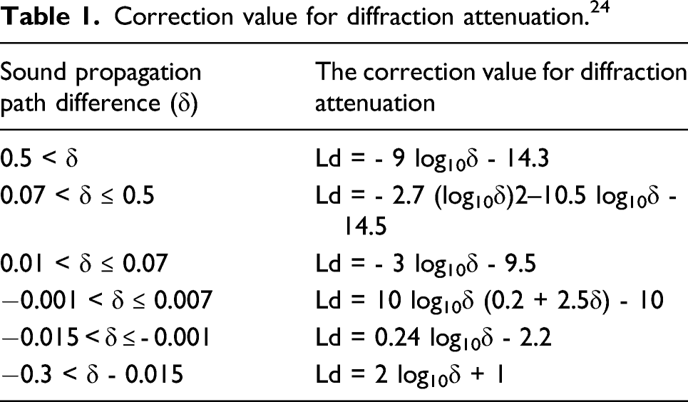
Then, the equation for actual calculation becomes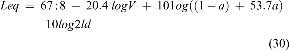

\begin{matrix} L e q = 67 : 8 + 20.4 l o g V + 101 o g ((1 - a) + 53.7 a) - 10 l o g 2 l d \end{matrix}

(30)

Burgess model

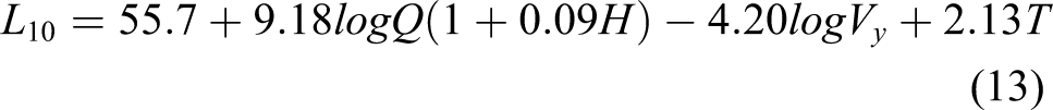
This model was developed at the National Physical Laboratory,²⁵ for Sydney Metropolitan Area. Factors considered during the measurements were traffic was free-flowing with no signal; the roadway was level, with the microphone set at 9 m away from the middle of the road; no shielding at a distance of 20 m was considered from parked vehicles and parks; and along the path of measurement, the microphone was set 10 m away from the nearest reflecting surface. Measurements of vehicle flow, speed, and noise were recorded for 10 min. The predicted L₁₀ formula is thus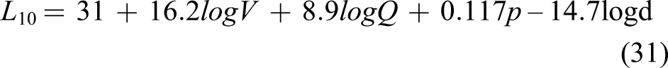

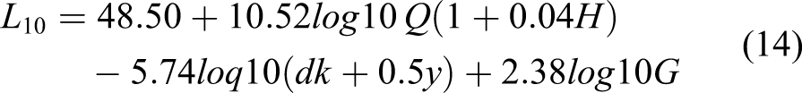
\begin{matrix} L_{10} = 31 + 16.2 l o g V + 8.9 l o g Q + 0.117 p - 14.7 l o g d \end{matrix}

(31)

where

V

= average speed (km/h),

Q

= total number of vehicles,

p

= percentage of heavy vehicles, and

d

= distance.

As comparisons between the measured and predicted measurement were above the permissible range, a modified model was developed

\begin{matrix} L_{10} = 56 + 10.7 l o g Q + 0.3 p - 18.5 l o g d \end{matrix}

(32)

The above formula did not consider average speed, as it was assumed that most vehicles were traveling at a steady speed when passing through the measurement point. The omission of $V$ from the formula revealed a high coefficient correlation value of 0.93 indicating the inclusion of vehicle speed invalid.

Further analysis was carried to develop an equivalent noise level equation as this is also an assessment for road noise annoyance and is widely used and accepted. This also gave a satisfactory correlation value of 0.95 with a standard error of 1.5 dB(A) when compared with measured Leq. The $L e q$ formula developed was of the form

\begin{matrix} L e q = 55. + 10.2 l o q Q + 0.3 p - 19.3 l o g d \end{matrix}

(33)

Nevertheless,²⁵ we concluded that heavy vehicles added to the noise levels of traffic, and the removal of speed minimized errors and simplified the model. Hence, the $L_{e q}$ and $L_{10}$ models are effective for uninterrupted traffic in Australia.

British Standard (BS-5228)

This section of BS-5228 sets guidance on methods to predict and quantify noise and determine its effect on those who are subjected to it. The prediction of equivalent continuous sound level for earthmoving machinery (mobile plant) that travels at intervals along the road, most times during construction, is achieved by calculating Leq using the following method²⁶:

The expression for Leq is given by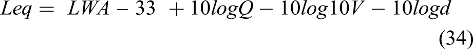

\begin{matrix} L e q = L W A - 33 + 10 l o g Q - 10 l o g 10 V - 10 l o g d \end{matrix}

(34)

where

L W A

=sound power level of the plant dB(A),

Q

=number of veh/hr,

V

=average speed of the vehicle (km/h), and

d

= distance from the center of the roadway to the receiving point of measurement. The following estimates are made: adjustments of

L e q

for reflections/screening if the receiving point is 1m from a building by adding or subtracting to the equation and when the angle view of the road is less than 180°, the below expression is applicable

\begin{matrix} A = 10 l o g (a / 180) \end{matrix}

(35)

where

A

=angle adjustment/correction and

a

=angle view of the road.

Adjustments for the nature of the ground over which the sound is propagated are also calculated. The ground is classified as soft, hard, or mixed. If the distance $R$ , in meters (m), from the point of interest to the geometric center of the plant or activity is other than 10 m, by applying the following equation

\begin{matrix} K h = 20 l o g R / 10 \end{matrix}

(36)

\begin{matrix} K s = (25 l o g R / 10) - 2 \end{matrix}

(37)

where

K s

= distance adjustment for soft ground;

K h

= distance adjustment for hard ground; and

R

≥ 25 m. For mixed ground, the calculation is according to proportion; for example, for 10% hard ground, and at a height of 2.5 m above ground level, adjustment is

\begin{matrix} 0.10 (k h - k s) \end{matrix}

(38)

ISO 9613

ISO (International Standardization Organization) is a global network of standard bodies. This aspect of ISO 9613 explicitly states an engineering method for determining sound attenuation during outdoor propagation to predict noise levels at a distance from a myriad of different sources which may be in motion or static. The sound propagation effects are geometrical divergence, atmospheric absorption, ground effect, reflection from surfaces, and screening by obstacles.

The equivalent sound pressure level at the receiver, in downwind conditions, is calculated for each point source based on the formula

\begin{matrix} L_{e q} (D W) = L_{w} + D_{c} - A \end{matrix}

(39)

where

L_{e q} (D W)

is the equivalent sound pressure level at the receiver, in downwind conditions, for octave bands;

L_{w}

is the sound power level by the point source;

D_{c}

is the directivity correction that describes the deviation of the sound pressure level in a specific direction from the sound power level; and

A

is the attenuation of the sound propagation given as

\begin{matrix} A_{d i v} + A_{a t m} + A_{g r} + A_{b a r} + A_{m i s c} \end{matrix}

(40)

It is a sum of the attenuation due to the geometrical divergence, the atmospheric absorption, the ground effect, the barriers, and miscellaneous other effects. The geometrical divergence accounts for spherical spreading in the free field from a point sound source, making the attenuation in decibels as

\begin{matrix} A_{d i v} = 20 log (d / d_{0}) + 11 \end{matrix}

(41)

where

d

is the distance from the source to receiver, in meters, and do is the reference distance (= 1 m).

The sound attenuation due to atmospheric absorption $(A_{t m})$ is calculated based on the atmospheric absorption coefficient (α), according to the formula

\begin{matrix} A_{t m} = α d / 1000 \end{matrix}

(42)

The ground effect is mainly the reflection of the sound rays that interact with the direct rays. For terrains approximately flat or with a constant slope, it depends on the source of noise, the type of terrain, and the receiver height. Barrier attenuation is calculated for each octave band based on variants as the wavelength and meteorological effects.²⁷ For long periods, the meteorological correction is applied; in this case, the long-term average sound power ( $L T)$ level is calculated according to the formula from (ISO, 1996)

\begin{matrix} L_{e q} (L T) = L_{e q} (D W) - C_{m e t} \end{matrix}

(43)

where

L_{e q}

is the equivalent sound pressure level at the receiver and

C_{m e t}

is the meteorological correction.²⁷

Nordtest

The approach defines exactly how to measure the noise level at a given position in a distinct way, and by determining road traffic noise all at once using several microphone positions, the noise levels in these positions can be efficiently figured out. By determining the traffic noise continually for a certain period, the equivalent noise level for that time can be identified directly.²⁸ The 24-h equivalent noise level L_Aeq,24h can be identified based on a complete 24-h measurement. If the noise levels during the day, evening, and night are identified independently, L_Aeq,24h can be figured out by making use of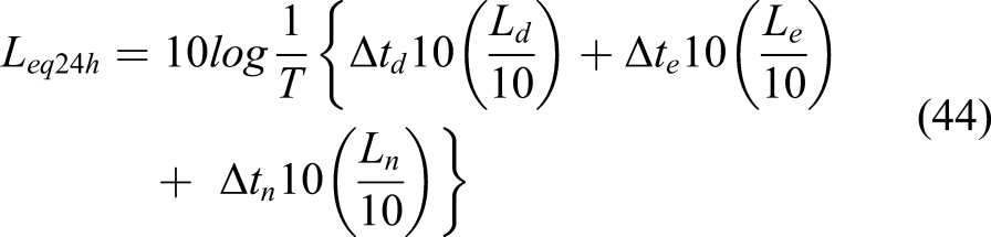

\begin{matrix} L_{e q 24 h} = 10 l o g \frac{1}{T} {Δ t_{d} 10 (\frac{L_{d}}{10}) + Δ t_{e} 10 (\frac{L_{e}}{10}) + Δ t_{n} 10 (\frac{L_{n}}{10})} \end{matrix}

(44)

where

T = Δ t d + Δ t e + Δ t n = 24 hours

L_{d}

L_{e}

, and

L_{n}

are the equivalent noise levels measured for the day

(Δ t d)

, evening

(Δ t e)

, and night

(Δ t n)

time interval, respectively.

As an option to measuring throughout the entire day, night, or evening period, measured noise levels from the traffic passing throughout the measurement period can be converted to correspond to average traffic conditions. This conversion can be made by using the below equations:

Heavy vehicles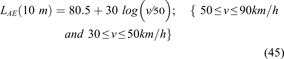

\begin{matrix} L_{A E} (10 m) = 80.5 + 30 l o g (\frac{v}{50}); {50 \leq v \leq 90 k m / h a n d 30 \leq v \leq 50 k m / h} \end{matrix}

(45)

Light vehicles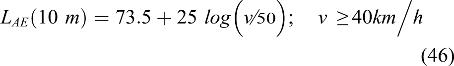

\begin{matrix} L_{A E} (10 m) = 73.5 + 25 l o g (\frac{v}{50}); v \geq 40 k m / h \end{matrix}

(46)

\begin{matrix} L_{A E} (10 m) = 71.1 + 25 l o g (\frac{10}{50}); 30 \leq v < 40 k m / h \end{matrix}

(47)

Finally, the equivalent noise level calculation is given by

\begin{matrix} L_{A e q, 1 h} (10 m) = 10 l o g \frac{1}{3600} {n_{h e a v y} 10 (\frac{L_{A e, h e a v y}}{10}) + n_{l i g h t} 10 (\frac{L_{A e, l i g h t}}{10})} \end{matrix}

(48)

where

n_{h e a v y}

and

n_{l i g h t}

are the average numbers per hour of heavy and light vehicles, respectively, in the traffic flow. It is assumed that the model depicts the daily standard vehicle noise emission together with the driving conditions.

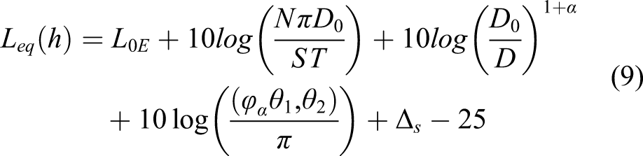
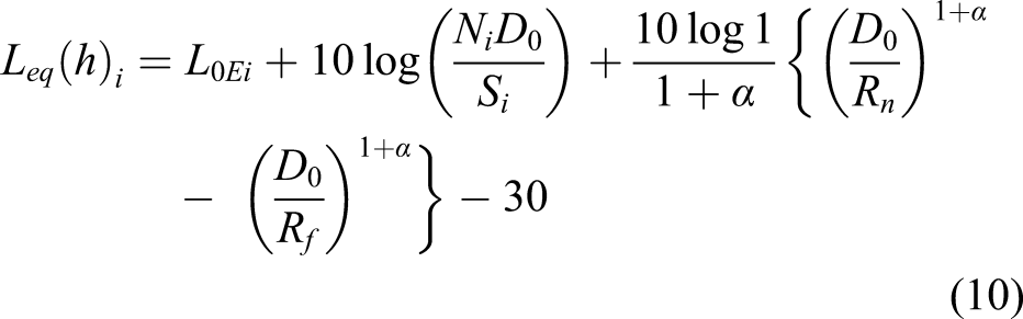
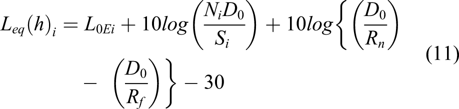
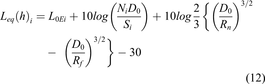
Acoustical Society of Japan model

The Acoustical Society of Japan (ASJ) RTN-models are used to design environmental preservation measures (noise abatement measures) and to estimate the current state of noise during environmental monitoring (regular observation). The model is based on certain conditions: type of road (pavement, geometry, and signalized/unsignalized), traffic volume, running speed of vehicles (for steady and non-steady flow), prediction range (length of roadway and height of measurement above the ground), and meteorological conditions.^29,30

The sound power level of road vehicles generally varies with the vehicle speed, engine rotational speed, and engine load.³¹ The ASJ sound power level model is given simply as a function of the vehicle speed, though the change in the noise generated due to the pavement type, road gradient, and noise directivity is considered in the correction terms. The A-weighted sound power level of a road vehicle (L_wA) is given by

\begin{matrix} L_{w A} = a + b l o g V + C \end{matrix}

(49)

where

L_{w A}

is the sound power level (dB)A,

V

is the vehicle speed (km/h),

a

and

b

are regression coefficients, and

C

is the correction for a different change in the noise radiation. Two cases are proposed for the values of

a

and

b

For steady flow steady traffic flow section (a section of the expressway or general road and without or distant from signalized intersections), with vehicle speed $V$ in the range from 40 to 140 km/h

\begin{matrix} L_{w A} = a + 30 l o g V + C \end{matrix}

(50)

Non-steady traffic flow section (general road including signalized intersections), with vehicle speed V in the range from 10 to 60 km/h

\begin{matrix} L_{w A} = a + 10 l o g V + C \end{matrix}

(51)

The values of coefficients in equation (51) are provided in Ref. [29] separately for sections of steady and non-steady traffic flow according to the different classes of vehicle.

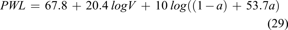
CNOSSOS-EU method

This research analyzes recorded data of road traffic simulations of the equivalent sound level. The CNOSSOS-EU model aimed to establish long-term indicators for a year. Toward this purpose, traffic noise and vehicle control systems were mounted in certain locations utilizing fixed surveillance devices to capture the measuring values all through the year.³² Vehicles were categorized into four classes (1-light motor vehicles, 2-medium-heavy vehicles, 3-heavy vehicles, and 4-powered two-wheelers). Sound level emissions are categorized as: propulsion (exhaust systems or engine noise) and tire–road interaction (rolling noise).³³

The propulsion sound power level from the Cnossos-EU model is given by

\begin{matrix} L_{W P, i, m} (V_{m}) = A_{P, i, m} + B_{P, i, m} + (\frac{V_{m} . V_{r e f}}{V_{r e f}}) + Δ L_{W P, i, m} \end{matrix}

(52)

where

i

is number of octave bands;

m

is classes of vehicles;

V_{m}

is speed from tire–road interaction, of

m

;

V_{r e f}

is reference speed =70 km/h;

A_{P, i, m}

B_{P, i, m}

is coefficient for each octave band and each vehicle category; and

Δ L_{W P, i, m}

is adjustments coefficients.

Rolling sound power level

\begin{matrix} L_{W R, i, m} (V_{m}) = A_{R, i, m} + B_{R, i, m} l o g (\frac{V_{m}}{V_{r e f}}) + Δ L_{W R, i, m} \end{matrix}

(53)

where

A_{R, i, m}

B_{R, i, m}

is coefficient for each octave band and each vehicle category at the reference conditions and

Δ L_{W R, i, m}

is adjustment coefficients. The sound power level of the traffic stream was represented as a line source and the average speed

(V_{m})

for all free-flowing vehicles steady traffic flow of vehicles estimated by

\begin{matrix} L_{W e q i, m} = L_{W, i, m} (V_{m}) + 10 l o g (\frac{Q_{m}}{1000. V_{m}}) \end{matrix}

(54)

where

Q_{m}

= total volume and speed =

V_{m}

Environmental noise guidelines

In view of the unprecedented increase in pollution from environmental noise, some countries and organizations have established allowable noise levels for the reduction of noise from road traffic. Some of these are discussed below:

World health organization

The World Health Organization (WHO) examined the evaluation of noise pollution and its effects on inhabitants and developed a standard environmental guideline.³⁴ Table 2 illustrates the WHO guidelines values for community noise.

Table 2.

World Health Organization community noise guidelines.

Environment	Critical health Effect(s)	Sound level dB(A)	Time (hours)
Outdoor living areas	Serious annoyance	50	16
Outdoor living areas	Moderate annoyance	55	16
Indoor dwellings	Speech intelligibility/Moderate annoyance	35	16
Bedrooms	Sleep disturbance	30	8
School classrooms	Disturbance of communication	35	During class
Pre-school bedrooms	Sleep disturbance	30	Sleeping time
School, playground	Annoyance (external source)	55	During playtime
Hospital, wardrooms	Sleep disturbance, night time	30	8
Hospital, wardrooms	Sleep disturbance, daytime/evening	30	16
Hospital, treatment rooms	Interference with rest/recovery	As low as possible
Industrial, commercial and traffic areas	Hearing impairment	70	24
Music through earphones	Hearing impairment	85	1
Ceremonies and entertainment	Hearing impairment	100	4

Source:³⁴

Nordic method

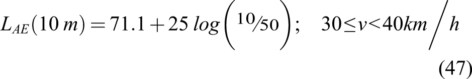
This method was developed by the Nordic group of experts to predict roadway noise in Nordic country³⁵ with road surface pavement dry and free from snow or ice. It is mainly designed to predict noise in front of a façade and can also be applied for indoor noise measurements. Measurement of the sound exposure level (L_Ae) developed was a function of average speed taken at10 m from the centerline of the road; vehicles were classified as light (<3.5 tons) and heavy vehicles (>3.5 tons). The effect of dispersion of noise was based on the fact that noise travels 0.5 m above the road surface from source to receiver and the sound-absorbing effect between source and receiver varies according to the type of road surface; this they classified as hard ground (asphalt, concrete, and soil with no vegetation) and soft ground (soil with vegetation) .³⁵ In this method, noise from tire–road interaction is not included as the speed of test vehicles was driving on full acceleration <50 km/h indicating a driving situation where the engine sound is the dominant sound source. And so, noise from vehicular speed >60 km/h cannot be applied to this method.

To describe the fluctuating noise, the A-weighted energy equivalent continuous sound pressure level over a 24-h period L_Aeq,24 is used for practical purposes as dose-response relation between the percentage of people feeling very annoyed by road noise and the outdoor noise level. Based on this, the noise guidelines were developed; these guidelines are defined as “free field” for L_Aeq,24 levels measured from 1 m in front of the facade or recreational areas (Table 3).³⁵

Table 3.

Free field noise guidelines.

Zones	Noise limits
Recreational areas in open country	50 dB
Recreational areas in towns/Residential areas	55 dB–65 dB
Public institutions	55 dB
Trade and commerce	60 dB–70 dB

These guidelines are used as standards in land use planning for new roads but are not used in relation to existing roads and existing homes.

The US Federal Highway Administration (FHWA)

The FHWA agency analyses traffic noise impacts based on proposed or envisaged road projects by evaluating measurements from the field and from existing projects by annually predicting and planning for traffic noise impacts. These impacts were grouped for different categories (A-G) based on exterior activities, as shown in Table 4.

Table 4.

The US Federal Highway Administration (FHWA) noise standard.

Activity category	Noise level (L_eq(h))	Noise Level L₁₀	Evaluation location	Description of land use category
A	57	60	Exterior	Lands on which serenity and quiet are of extraordinary significance
B^1,a	67	70	Exterior	Residential area
C^a	67	70	Exterior	Hospitals, schools, libraries, hospitals, places of worship etc.
D	52	55	Interior	Places of worship, hospitals, day-care centers, libraries, schools, etc.
E^a	72	75	Exterior	Hotels, bars, etc
F	––	––	––	Airports, bus yards, emergency services, maintenance facilities, manufacturing, etc.
G	––	––	––	Undeveloped lands that are not permitted

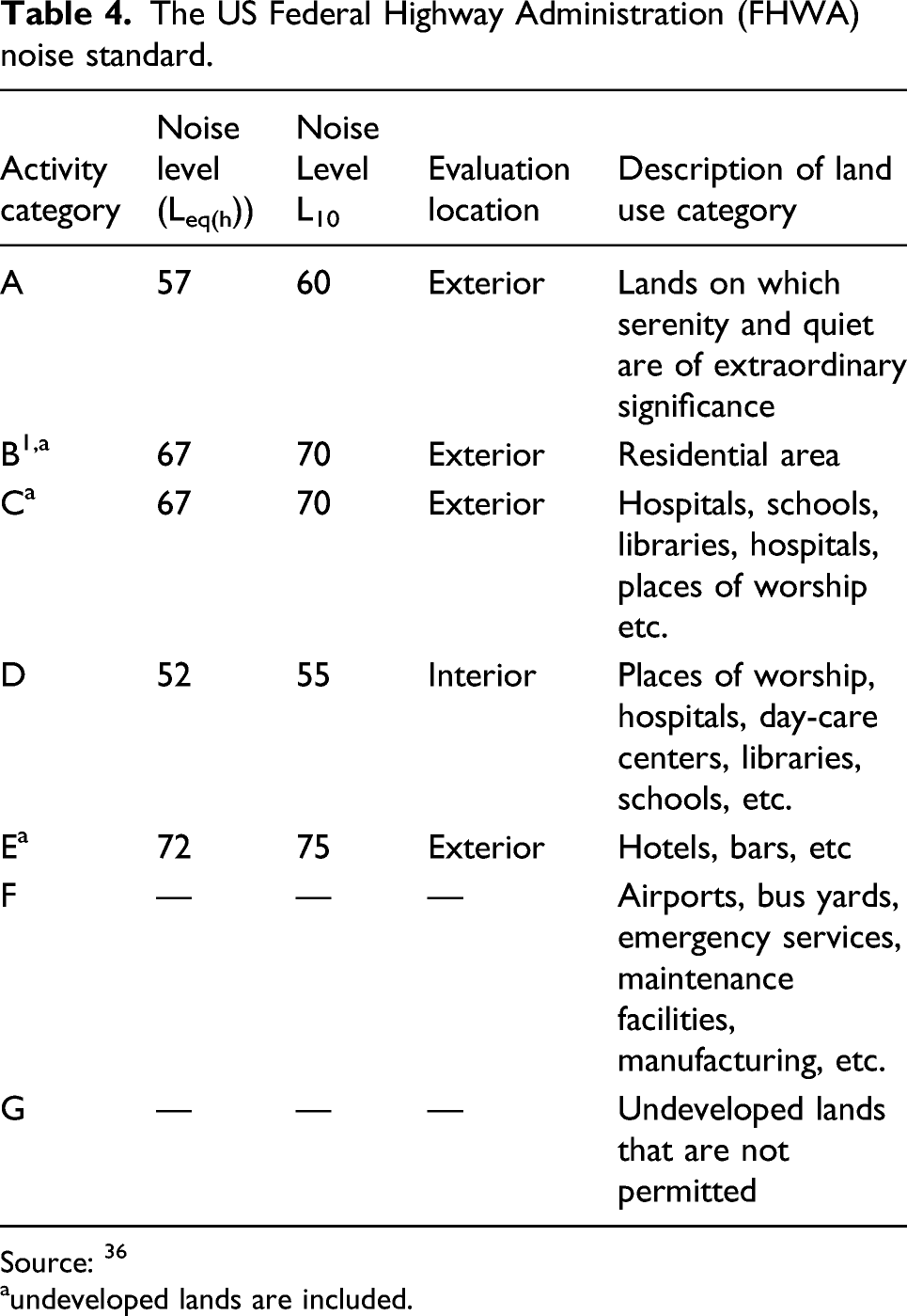
Source: ³⁶

^aundeveloped lands are included.

The Leq(h) and L₁₀(h) activity criteria values are for impact determination only and are not design standards for noise abatement measures and either of them (but not both) may be used on a project.

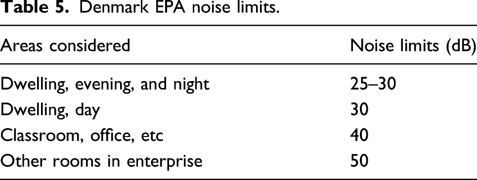
Denmark environmental protection agency

Denmark established limit values for environmental noise. These limits are given as A-weighted and are associated with the sound levels measured with reference periods of 8 h, 1 h, and 30 min for the day, the evening, and the night period, respectively.³⁷ Table 5 is the Denmark Environmental Protection Agency (EPA) permissible noise limits.

Table 5.

Denmark EPA noise limits.

Areas considered	Noise limits (dB)
Dwelling, evening, and night	25–30
Dwelling, day	30
Classroom, office, etc	40
Other rooms in enterprise	50

Discussion

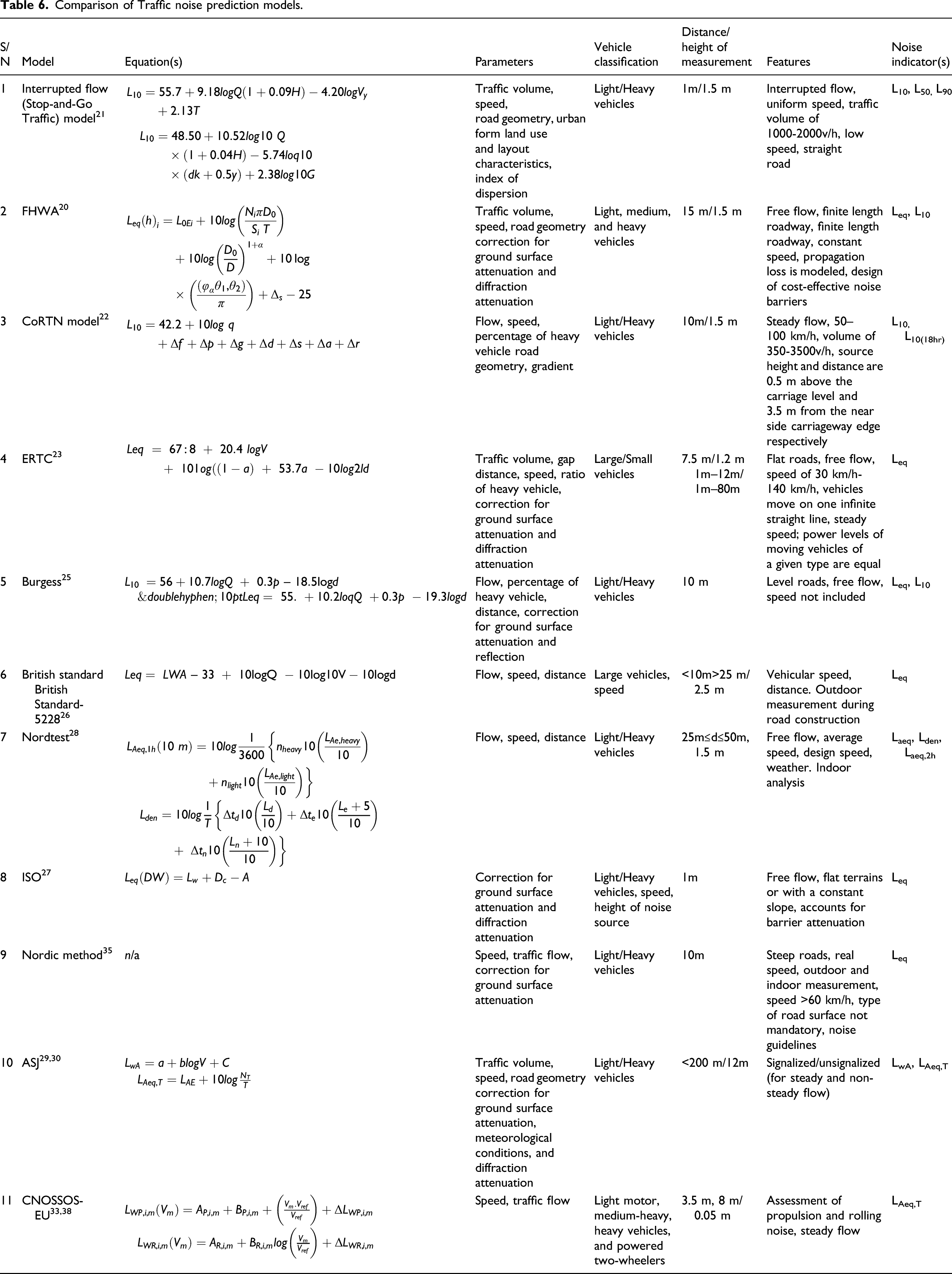
The findings from the reviewed articles revealed that traffic noise models are developed to assess and predict traffic noise to mitigate the environmental impacts it has on the inhabitants. It is important to study the causes and effects of noise in terms of its indicators ( $L_{e q}, L_{10}$ , etc.) by evaluating the factors associated with the traffic noise level. The following models: FHWA, Stop-and-Go, Burgess, ERTC, CoRTN and British Standard (BS), Nordic methods, Nordtest, ISO 9613, and ASJ Model CNOSSOS-EU have their peculiarities. The Burgess and Stop-and-Go models consider interrupted traffic flow while the CoRTN, FHWA, and other models (BS, ERTC, CNOSSOS-EU, and Nordtest) assume a uniform speed for all vehicular traffic though accounts for ground attenuation.

In its performance, the Burgess model remains suitable as a measure explaining the distribution of noise caused by social groups, land use, and urban growth within urban areas. In the FHWA model, vehicles are classified into light commercial vehicles, medium trucks, and heavy trucks. These vehicles are expected to traverse flat roads with constant velocity. As a result, no separate acceleration or deceleration lanes are incorporated, unlike the CNOSSOS-EU method.

For the Interrupted Stop-and-Go model, vehicles are classified as light or heavy. The flow of these vehicles in the traffic stream is continuously interrupted. The model assumes a straight road with a good surface condition on which vehicles traverse with a steady uniform speed of traffic.

This is not the case for FHWA and CoRTN noise models which consider free flow and steady flow of vehicles, respectively. CoRTN allows no adjustment for downhill driving conditions in terms of terrain because the technique does not take into account engine braking noise often emitted by heavy vehicles while descending. The model allows curve fitting of measured data in which the parameters of source emission and sound propagation are organized in graphic format to provide a reasonably simple prediction method.

ASJ, Nordtest, and Nordic consider both outdoor and indoor effects of traffic noise level on inhabitants. ASJ model is applicable for light and heavy vehicles at signalized and unsignalized intersections with the steady and non-steady flow. However, the Nordic noise model is applicable for light and heavy vehicles moving with a speed not more than 60kmh along steep roads and proves to be more effective in correcting ground surface attenuation, while the Nordtest method is best suited for light and heavy vehicles moving at free flow with average speed.

ISO and other noise models capture the outdoor effect of traffic noise level only. It is best suited for free flow moving vehicles on flat terrains or with a constant slope and accounts for barrier attenuation. One limitation that makes it impracticable in practice is that the standard estimates only moderate downwind conditions when defining atmospheric attenuation. Another drawback is that, within 1 km, the standard only provides approximate accuracy. This implies that forecasts beyond 1 km will significantly vary from the results measured.

From these models developed by different countries, it is evident that they account for traffic noise conditions, from the source of sound propagation to the receptor in relation to traffic conditions, meteorological conditions, diffraction, and adsorption. The indoor–outdoor sound propagation under a complex environment has been a vital issue of research for improving the accuracy of traffic noise models. Generally, most of these models developed predicted for

L_{e q}

and

L_{10}

indicators. Table 6 summarizes the models that were reviewed.

Table 6.

Comparison of Traffic noise prediction models.

S/N	Model	Equation(s)	Parameters	Vehicle classification	Distance/height of measurement	Features	Noise indicator(s)
1	Interrupted flow (Stop-and-Go Traffic) model²¹	$L_{10} = 55.7 + 9.18 l o g Q (1 + 0.09 H) - 4.20 l o g V_{y} + 2.13 T$ $L_{10} = 48.50 + 10.52 l o g 10 Q (1 + 0.04 H) - 5.74 l o q 10 (d k + 0.5 y) + 2.38 l o g 10 G$	Traffic volume, speed, road geometry, urban form land use and layout characteristics, index of dispersion	Light/Heavy vehicles	1m/1.5 m	Interrupted flow, uniform speed, traffic volume of 1000-2000v/h, low speed, straight road	L₁₀, L_50, L₉₀
2	FHWA²⁰	$L_{e q} {(h)}_{i} = L_{0 E i} + 10 l o g (\frac{N_{i} π D_{0}}{S_{i} T}) + 10 l o g {(\frac{D_{0}}{D})}^{1 + α} + 10 \log (\frac{(φ_{α} θ_{1}, θ_{2})}{π}) + Δ_{s} - 25$	Traffic volume, speed, road geometry correction for ground surface attenuation and diffraction attenuation	Light, medium, and heavy vehicles	15 m/1.5 m	Free flow, finite length roadway, finite length roadway, constant speed, propagation loss is modeled, design of cost-effective noise barriers	L_eq, L₁₀
3	CoRTN model²²	$L_{10} = 42.2 + 10 l o g q + Δ f + Δ p + Δ g + Δ d + Δ s + Δ a + Δ r$	Flow, speed, percentage of heavy vehicle road geometry, gradient	Light/Heavy vehicles	10m/1.5 m	Steady flow, 50–100 km/h, volume of 350-3500v/h, source height and distance are 0.5 m above the carriage level and 3.5 m from the near side carriageway edge respectively	L_10, L_10(18hr)
4	ERTC²³	$L e q = 67 : 8 + 20.4 l o g V + 101 o g ((1 - a) + 53.7 a - 10 l o g 2 l d$	Traffic volume, gap distance, speed, ratio of heavy vehicle, correction for ground surface attenuation and diffraction attenuation	Large/Small vehicles	7.5 m/1.2 m 1m–12m/1m–80m	Flat roads, free flow, speed of 30 km/h-140 km/h, vehicles move on one infinite straight line, steady speed; power levels of moving vehicles of a given type are equal	L_eq
5	Burgess²⁵	$L_{10} = 56 + 10.7 l o g Q + 0.3 p - 18.5 l o g d$ $L e q = 55. + 10.2 l o q Q + 0.3 p - 19.3 l o g d$	Flow, percentage of heavy vehicle, distance, correction for ground surface attenuation and reflection	Light/Heavy vehicles	10 m	Level roads, free flow, speed not included	L_eq, L₁₀
6	British standard British Standard-5228²⁶	$L e q = L W A - 33 + 10 l o g Q - 10 l o g 10 V - 10 l o g d$	Flow, speed, distance	Large vehicles, speed	<10m>25 m/2.5 m	Vehicular speed, distance. Outdoor measurement during road construction	L_eq
7	Nordtest²⁸	$L_{A e q, 1 h} (10 m) = 10 l o g \frac{1}{3600} {n_{h e a v y} 10 (\frac{L_{A e, h e a v y}}{10}) + n_{l i g h t} 10 (\frac{L_{A e, l i g h t}}{10})}$ $L_{d e n} = 10 l o g \frac{1}{T} {Δ t_{d} 10 (\frac{L_{d}}{10}) + Δ t_{e} 10 (\frac{L_{e} + 5}{10}) + Δ t_{n} 10 (\frac{L_{n} + 10}{10})}$	Flow, speed, distance	Light/Heavy vehicles	25m≤d≤50m, 1.5 m	Free flow, average speed, design speed, weather. Indoor analysis	L_aeq, L_den, L_aeq,2h
8	ISO²⁷	$L_{e q} (D W) = L_{w} + D_{c} - A$	Correction for ground surface attenuation and diffraction attenuation	Light/Heavy vehicles, speed, height of noise source	1m	Free flow, flat terrains or with a constant slope, accounts for barrier attenuation	L_eq
9	Nordic method³⁵	n/a	Speed, traffic flow, correction for ground surface attenuation	Light/Heavy vehicles	10m	Steep roads, real speed, outdoor and indoor measurement, speed >60 km/h, type of road surface not mandatory, noise guidelines	L_eq
10	ASJ^29,30	$L_{w A} = a + b l o g V + C$ $L_{A e q, T} = L_{A E} + 10 l o g \frac{N_{T}}{T}$	Traffic volume, speed, road geometry correction for ground surface attenuation, meteorological conditions, and diffraction attenuation	Light/Heavy vehicles	<200 m/12m	Signalized/unsignalized (for steady and non-steady flow)	L_wA, L_Aeq,T
11	CNOSSOS-EU^33,38	$L_{W P, i, m} (V_{m}) = A_{P, i, m} + B_{P, i, m} + (\frac{V_{m} . V_{r e f}}{V_{r e f}}) + Δ L_{W P, i, m}$ $L_{W R, i, m} (V_{m}) = A_{R, i, m} + B_{R, i, m} l o g (\frac{V_{m}}{V_{r e f}}) + Δ L_{W R, i, m}$	Speed, traffic flow	Light motor, medium-heavy, heavy vehicles, and powered two-wheelers	3.5 m, 8 m/0.05 m	Assessment of propulsion and rolling noise, steady flow	L_Aeq,T

Conclusion

To be able to develop strategies to mitigate the negative consequences of traffic noise, it is important to understand how to measure it. As such, the analysis of traffic noise requires some theoretically consistent quantitative techniques that may be transferable or adjustable to local conditions. In this study, 11 traffic noise models from different parts of the world were reviewed. It was observed that researchers from different countries have developed traffic noise prediction models by adopting some of the earlier models as a baseline or replicating, and testing them for their applicability and reliability in predicting roadway noise based on their underlying local traffic conditions. This has particularly been the case due to costs and time involved in developing new traffic noise models.

This comprehensive review of traffic noise modeling strategies has revealed that prior to recent data-driven noise reduction efforts, the effective methods and control procedures of traffic noise were to reduce the noise emission from the source, noise control within the sound transmission path, protection at the receiving end, land use planning, education, and public awareness. In recent years, studies have shown that with integrated noise permissible limits and regulation, policies need to be fully implemented for noise amelioration. This is because traffic noise assessment and evaluation can enhance urban planning for envisaged road networks and possibly help in curbing noise pollution on existing traffic corridors, thereby ensuring the safety of the inhabitants and sustainability of the environment.

Therefore, it is recommended that the current noise guidelines be revised and updated because they are obsolete as there has been a rise in automobile traffic, population, urbanization, etc. in cities. Furthermore, for further analysis, traffic noise modeling should include examining and analyzing different noise emissions from vehicle components, such as the horn, exhaust, etc. In addition, noise assessments also should be carried out during road construction and maintenance as transport projects are not only assessed on their economics and characteristics but also on their impacts. These could therefore identify the significant factors leading to noise generation and thus promote mitigation processes for sustainable roadway infrastructure.

Footnotes

Declaration of conflicting interests

The author(s) declared no potential conflicts of interest with respect to the research, authorship, and/or publication of this article.

Funding

The author(s) disclosed receipt of the following financial support for the research, authorship, and/or publication of this article: This work was supported by Regional Transport Research Education Centre, Kumasi

ORCID iD

Fidelma Ibili

Notations

dB	Decibel
L_eq	Equivalent sound level
L_n	n-Percent exceeded level
NPL	Noise pollution level
TNI	Traffic noise index
NC	Noise climate
dB(A)	A-weighted decibel
v, N	Speed
C	Engine capacity
l_m	Maximum noise level
l_w	Acoustic power
d	Distance
FHWA	Federal highway administration
Q, q	Traffic volume
H, p	Proportion of heavy vehicle
CoRTN	Calculation of road traffic noise model
f	Volume of heavy vehicle per hour
PWL	A-weighted energy average power level of vehicle
L_WA	Weighted sound power level
a	Angle view of the road
C_met	Meteorological correction
m	Classes of vehicle
HP	Horse power

References

Bhardwaj

Aggarwal

Bhardwaj

. A review on impacts of road activities and vehicular emissions on native ecosystems in mountainous region. Curr World Environ 2019; 14: 194–204.

Pachiappan

Govindaraj

. Regression modelling of traffic noise pollution. Građevinar 2013; 65: 1089–1096.

Ozer

Yilmaz

Yeşil

, et al. Evaluation of noise pollution caused by vehicles in the city of Tokat, Turkey. Sci Res Essays 2009; 4: 1205–1212.

Wallas

Ekström

Bergström

, et al. Traffic noise exposure in relation to adverse birth outcomes and body mass between birth and adolescence. Environ Res 2019; 169: 362–367.

Christensen

Hjortebjerg

Raaschou-Nielsen

, et al. Pregnancy and childhood exposure to residential traffic noise and overweight at 7 years of age. Environ Int 2016; 94: 170–176.

Trivedy

. Encyclopedia of environmental pollution and control. Austin, TX: Enviro Media, 1995.

Kumar

KVD

Srinivas

. Study of noise levels at commercial and industrial areas in an urban environment. J Eng Res Appl 2015; 5(10): 89–92.

Ramalingeswara Rao

Seshagiri Rao

. Urban traffic intensity: a prediction of (Leq) noise levels. Ind J Environ Health 1991; 33: 324–329.

Tian

, et al. Assessment of traffic noise pollution from 1989 to 2003 in Lanzhou city. Environ Monit Assess 2006; 123: 413–430.

10.

Oyedepo

Adeyemi

Olawole

, et al. A GIS - based method for assessment and mapping of noise pollution in Ota metropolis, Nigeria. MethodsX 2019; 6: 447–457.

11.

Pathak

Tripathi

Mishra

. Dynamics of traffic noise in a tropical city Varanasi and its abatement through vegetation. Environ Monit Assess 2008; 146: 67–75.

12.

Annecke

Berge

Crawshaw

, et al. Noise reduction in urban areas from traffic and driver management. Report to European Commission Silence Project 2008.

13.

Sandberg

. Tyre/road noise: myths and realities. Linköping, Sweden: Statens väg-och transport forskningsinstitut, 2001.

14.

Rochat

Reiter

. Highway traffic noise. Acoust Today 2016; 12: 38–47.

15.

Federal Highway Administration . Highway traffic noise: analysis and abatement guidance, 75. Washington, DC: Federal Highway Administration, 2011.

16.

Priede

. The problems of noise of engines in different vehicle groups. SAE Tech Pap 1975; 84: 1963–1974.

17.

Steele

. A critical review of some traffic noise prediction models. Appl Acoust 2001; 62: 271–287.

18.

Priede

. Origins of automotive vehicle noise. J Sound Vibration 1971; 15: 61–73.

19.

Favre

Gras

. Noise emission of road vehicles: reconstitution of the acoustic signature. J Sound Vib 1984; 93: 273–288.

20.

Barry

Regan

. Fhwa highway traffic noise. Washington DC: USDOT - FHWA, 1979.

21.

Gilbert

. Noise from road traffic (interrupted flow). J Sound Vibration 1977; 51: 171–181.

22.

Dept.of Transport . Calculation of road traffic noise. London, UK: Her Majesty’s Stationery Office, 1988.

23.

Suksaard

Sukasem

Tabucanon

, et al. Road traffic noise prediction model in Thailand. Appl Acoust 1999; 58: 123–130.

24.

Ishii

. Prediction of road traffic noise (part 1), method of practical calculation. J Acoust Soc Jpn(J) 1975; 31: 507–517.

25.

Burgess

. Noise prediction for urban traffic conditions-related to measurements in the Sydney Metropolitan Area. Appl Acoust 1977; 10: 1–7.

26.

BSI. British . Standards Code of Practice for noise and vibration control on. London, UK: BSI Standards Limited, 2014.

27.

ISO. Acoustics . Attenuation of sound during propagation outdoors. Markham, ON: ISO Acoustics, 1996, pp. 1–8.

28.

Nordtest . NT ACOU 056 Road traffic: measurement of noise immission – survey method, 1. Finland: Nordtest Organisation, 2002, pp. 1–9.

29.

Sakamoto

. Road traffic noise prediction model “ASJ RTN-Model 2013”: report of the research committee on road traffic noise. Acoust Sci Tech 2015; 36: 49–108.

30.

Yamamoto

. Road traffic noise prediction model “ASJ RTN-Model 2008”: report of the research committee on road traffic noise. Acoust Sci Tech 2010; 31: 2–55.

31.

Tsukui

Oshino

Tachibana

. Simulation model for road traffic noise taking account of vehicle noise directivity. J INCE Jpn 1998; 22: 108–116.

32.

Bakowski

Radziszewski

Dekys

, et al. Frequency analysis of urban traffic noise. In: Proc 2019 20th Int Carpathian Control Conf ICCC, Wieliczk, Poland, 26–29 May 2019. 2019; 10. Epub ahead of print 2019. DOI: 10.1109/CarpathianCC.2019.8766012.

33.

Kephalopoulos

Paviotti

Anfosso-Lédée

, et al. Advances in the development of common noise assessment methods in Europe: the CNOSSOS-EU framework for strategic environmental noise mapping. Sci Total Environ 2014; 482-483: 400–410.

34.

Berglund

Lindvall

Schwela

. Guidelines for community noise. World health organization. Noise Vib Worldwide 1995; 31: 1–141.

35.

Bendtsen

. The nordic prediction method for road traffic noise. Sci Total Environ 1999; 235: 331–338.

36.

FHWA Noise Standard . FHWA noise standard - 23 CFR 772. 109. Washington, DC: Federal Highway Administration, 2013.

37.

Jakobsen

. Danish guidelines on environmental low frequency noise, infrasound and vibration. J Low Frequen NoiseVib Active Cont 2001; 20: 141–148.

38.

Bakowski

. Validation of cnossos-EU urban traffic noise model. In: Proc 2019 20th Int Carpathian Control Conf ICCC 2019, Wieliczk, Poland, 26–29 May 2019. 2019; 4.

Traffic noise models and noise guidelines: A review

Abstract

Keywords

Introduction

Highway noise descriptors

Equivalent continuous sound level, Leq

The n-percent exceeded level, Ln

Noise pollution level

Traffic noise index (TNI)

Noise climate (NC)

Day, evening, and night equivalent noise level (Lden)

A-weighted decibels dB(A)

Factors contributing to traffic noise

Traffic factors

Road factors

Vehicle factors

Human factors

Traffic noise models

FHWA model

Interrupted flow (stop-and-go traffic) model

CoRTN model

ERTC model

Burgess model

British Standard (BS-5228)

ISO 9613

Nordtest

Acoustical Society of Japan model

CNOSSOS-EU method

Environmental noise guidelines

World health organization

Nordic method

The US Federal Highway Administration (FHWA)

Denmark environmental protection agency

Discussion

Conclusion

Footnotes

Declaration of conflicting interests

Funding

ORCID iD

Notations

References

The n-percent exceeded level, L_n

Day, evening, and night equivalent noise level (L_den)