Response surface model-based multi-objective optimization of Box–Behnken building design for indoor comfort and energy

Abstract

Rapid urbanization and the increasing energy demand of buildings necessitate modern building optimization techniques to maintain a suitable equilibrium between indoor comfort and building energy demand. This investigation aims to maintain an optimal balance between the building energy demand and indoor occupant comfort. Efforts have been made to optimize the independent variables influencing Indoor Environmental Quality (IEQ) response variables through a combination of advanced statistical and numerical techniques including the Box–Behnken design, response surface methodology (RSM), analysis of variance (ANOVA) and computational fluid dynamics (CFD). The statistically optimized solution obtained using RSM determined the optimal parameters: inlet diffuser inclination (IDI) = −76.52, inlet air velocity = 0.1 m/s, and radiator temperature = 300 K. The statistical model demonstrated strong reliability, with a mean root mean square error (RMSE) of 4.73% compared to numerical results with an R² of .998. The IDI appeared as the primary factor influencing building performance, with significant quadratic effects on operative temperature, indoor air velocity, and the predicted mean vote (PMV) index, highlighting precise modeling for indoor comfort assessment. The statistical methods applied in this study proved highly effective for numerical and experimental analyses. They hold significant potential for modeling indoor environments while addressing ventilation, air quality, thermal comfort, and energy efficiency.

Keywords

Thermal comfort response surface methodology statistical optimization computational fluid dynamics Box–Behnken

Introduction

Maintaining comfort in buildings requires up to 50% of total world-wide energy demand and is estimated to increase rapidly to 60% by 2050.^1,2 Heating, ventilation, and air conditioning (HVAC) systems account for significant energy demand in buildings and represent the rapidly demanding segments of energy.³ The average urban population spends about 90% of its time indoors, which demands a wide range of comfort requirements to improve indoor occupant productivity and health.⁴ This high demand for energy for residential and non-residential buildings contributes to climate change and global warming. Maintaining a proper balance between indoor comfort and building energy demand is crucial to moderate climate change by building more sustainable and efficient buildings.^5,6 In general, cross-ventilated buildings demonstrated a notable reduction in building energy demand ranging from 8 to 78% in cold, hot, and hot–humid climates depending on ambient air conditions.^7,8 Although a naturally ventilated building takes advantage of natural forces, it also limits indoor comfort in extreme seasonal weather conditions such as extremely cold and hot climates. In such situations, naturally ventilated buildings can be partially supported by mechanical equipment known as mixed ventilation buildings. The mixed-ventilated buildings combine the advantages of both naturally ventilated and mechanically ventilated buildings for optimal indoor comfort and energy demand.^9,10 Mixed-ventilated indoor environments are more favorable under cold climatic conditions and can reduce a considerable amount of energy with careful design of buildings while improving indoor comfort.¹¹ Mixed-ventilated indoor environments provide more well-regulated elements than pure natural or mechanical ventilation. The indoor air temperature (IAT), air velocity, humidity, ventilation location, inlet diffuser inclination (IDI), heating or cooling panels, and building envelope in mixed-ventilated buildings significantly influence building occupant comfort and heat load demand.^12–14 Maintaining a proper balance between these factors is challenging due to multiple control objectives to optimize indoor comfort and energy demand. The site of the inlet and outlet vents plays an important role in maintaining building comfort and contamination control. IDI is responsible for properly distributing fresh inlet air, which affects indoor comfort and energy demand. The formation of thermal stratification layers is affected due to ventilation location and IDI. An experimental study found that a significant impact on heating load was observed for different ventilation settings of naturally ventilated buildings.^15,16 Experimental and numerical studies show that if the exhaust vent is located near indoor occupants or at floor level, 20.8% decrease in heat load of the building can be observed.¹⁷ The selection of an appropriate IDI can affect IAT and fluid flow properties depending upon the different mixing patterns generated in the mixing zone near the radiator. Hence careful analysis of IDI is recommended for optimum indoor environment.^18,19 Symmetrical inlet vents or an aspect ratio of 4 enhance ventilation efficiency and control indoor contamination. The high velocity with a low effective aspect ratio increases the risk of indoor contamination due to the high concentration of carbon dioxide which ensures the need for efficient inlet aspect ratio design.^20,21 The study concludes that increasing the velocity has benefits in contamination removal but drastically increases the energy demand to achieve the targeted indoor comfort and contamination goals.²² The importance of the building envelope for indoor comfort and contamination control is critical while IDI can influence the building energy demand to maintain indoor comfort and contamination control.

In mixed-ventilated spaces, air movement is critical for maintaining indoor comfort. Higher indoor air movements and high air velocities in the vicinity of indoor occupants create a risk of cold air drafts in cold climate conditions. Air movement is a function dominated by IAT.²³ Velocity magnitude in mixed ventilated spaces should be limited to lower values (0.8 m/s), as suggested by many experimental and numerical studies.¹² In most observed studies, the velocity near occupants rarely exceeds 0.3 m/s in mechanically ventilated indoor spaces. In comparison, in naturally ventilated indoor environments, this magnitude should be 0.1 m/s for optimum occupant comfort.²⁴ In general, higher air speeds are acceptable at higher temperatures, while, under cold climatic conditions, this limit should be strictly adhered to for occupant comfort and to avoid cold air draft problems. A certain temperature allowance can be made for a slightly warmer, naturally ventilated indoor environments to avoid cold air drafts, as given by equation (1):^25,26

Δ T = 7 - \frac{50}{4 + 10 V_{a}^{0.5}}

(1)

where $Δ T$ is the permissible temperature and $V_{a}$ is the velocity of indoor air in a fluid domain (V_a ≥ 0.1 m/s)

The change in frequency of the air movement also influences the sensitivity to cold drafts and hence comfort. Higher eddies and circulations due to more intense air movement result in higher fluctuation frequency, and values higher than 0.5 Hz result in maximum draft intensity. The draft rating frequency depends on air temperature and air velocity which is given in equations (2) and (3):²⁷

D R = (34 - t_{a}) (V_{m e a n} - 0.05)^{0.62} (37. V_{r m s} + 3.14)

(2)

D R = (34 - t_{a}) (V_{m e a n} - 0.05)^{0.62} (0.37. V_{m e a n} . T_{u} + 3.14)

(3)

where $t_{a}$ (°C) is the temperature of indoor air, $T_{u} %$ is the turbulence, $V_{m e a n} (\frac{m}{s})$ is the mean velocity, and $V_{r m s} (\frac{m}{s})$ is the standard deviation of velocity fluctuation.

The airspeed for mechanically ventilated spaces should be less than 0.1 m/s, depending on the IAT.²⁸ Thus, finding the optimum velocity for optimal comfort and energy demand is essential for sustainable building development. Air velocity and the building envelope significantly affects the heating load on the radiator. The proper balance between these factors can considerably decrease the building heat load. The optimization of building parameters for energy and comfort needs multi-objective optimization techniques since these conflicting parameters are dependent on complex relationships. The performance of the existing, designed, and refurbished buildings for energy and comfort is collectively studied and known as building performance operation (BPO).^29,30 The conventional strategy analyses the influence of altered building parameters and their effect on building design by keeping all other parameters constant to enhance building heat load efficiency and performance. In general, these conventional methods use multiple numerical or experimental case studies to analyze the different factors independently. This repetitive methodology of trial and error makes analysis more complicated, costly, time-consuming, and practically impossible to carry out detailed parametric analysis.^31,32 The accuracy of the method depends on the complexity and the non-linearity of the dependent input variables.³³ The shortcomings of the conventional methods can be overcome by the BPO process by a combination of numerical and statistical methods. The numerical method which includes the modeling and simulation then combined with the mathematical or statistical methods can obtain the desired optimal solution.³³ This method can be used to minimize the number of numerical simulations and find the mathematical link among the multiple building responses.³⁴

The literature discussed above mentions the importance of the application of statistical methods along with numerical methods to optimize the multiple conflicting objectives in BPO since the parameters influencing indoor comfort and energy demand are conflicting in nature. This study analyses the influence of IDI, cold air inlet velocity, and radiator heating load on indoor comfort and building energy demand. Efforts have been made to establish the optimal trade-off between acceptable indoor occupant comfort and building heat load for a mixed-ventilated building. The combination of numerical method and statistical method has been used in this study to get the optimal values of parameters affecting the building comfort and performance. The predicted mean vote (PMV) index was analysed to study the indoor comfort. The building energy demand, the heating load on the radiator, was calculated for different IDIs and cold inlet air velocities. To reduce the number of simulations causing high computational cost and time, a multi-objective optimization method using design expert, RSM, and analysis of variance (ANOVA) has been employed. The study is organized into several key sections, including the physical model and methodology, the optimization of indoor environmental quality (IEQ) and energy demand, the results and discussion, the model optimization for IEQ, and the conclusions.

Physical problems and methodology

The indoor comfort and heating load on the radiator assumed to be mainly affected by the inlet air velocity, IDI, and radiator temperature under cold climatic conditions.^35–37 This study has attempted to analyze the shared influence of cold inlet air velocity, IDI, and radiator temperature on the building indoor comfort and heating load to retain acceptable occupant comfort. The advantages of numerical and statistical methods were used in the study to optimize the comfort and energy requirement variables. In the first step, the Box–Behnken method for design was used to generate various cases; in the next step, numerical simulations were performed using ANSYS Fluent; and in the third step, RSM was employed to optimize the multi-objective function of indoor comfort and energy requirements of the building. In the last step, the optimized design given by statistical method has been further verified with computational fluid dynamics (CFD) and analyzed for comfort and energy performance.

Physical model description

A cross- and mixed-ventilated, unoccupied building was designed using ICEM CFD software. This analysis has been carried out for cold climatic conditions, where the inlet air entering at 5°C at a constant velocity.

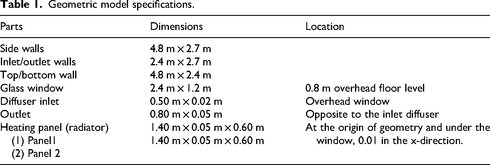
A double-panel heating radiator has been installed indoors to retain the comfort in the specified range. The geometric modeling of the building has dimensions of 4.8, 2.7, and 2.4 m of length, height, and width, respectively, with a fluid volume of 31.104 m³. All five walls of the room are considered adiabatic including the ceiling and floor to focus on indoor comfort and fluid flow analyses independent of ambient conditions. The radiator heating panel is located below the window and maintains the IAT with higher efficiency.³⁸ The geometric model consists of the inlet and outlet vents located on opposite walls. A glazed glass window above the radiator facilitates natural lighting in the indoor environment. A finely meshed geometric model is generated with targeted maximum mesh quality using a hexagonal mesh for more precise fluid flow analysis. The complete geometric design of the model is shown in Figure 1. The detailed geometric specifications of the numerical model are provided in Table 1.

Figure 1.

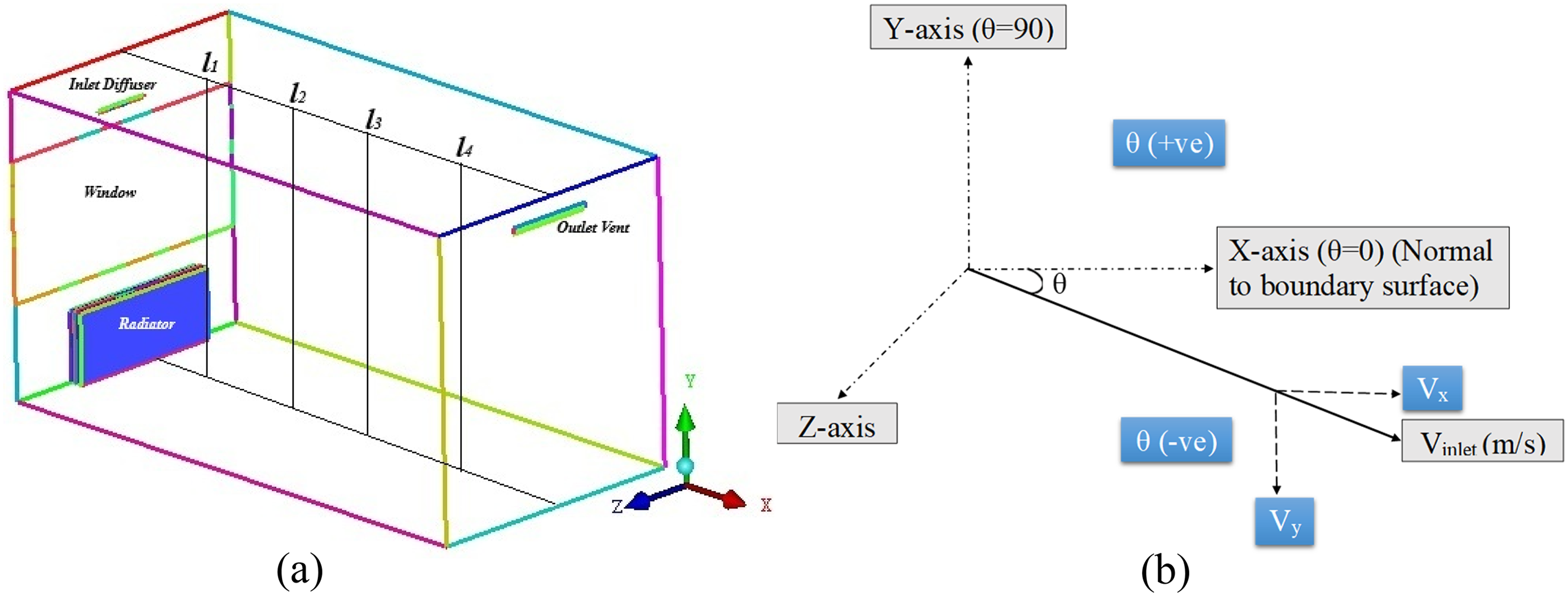
Numerical model. (a) Monitoring plane and lines, (b) IDI. IDI: inlet diffuser inclination.

Table 1.

Geometric model specifications.

Parts	Dimensions	Location
Side walls	4.8 m × 2.7 m
Inlet/outlet walls	2.4 m × 2.7 m
Top/bottom wall	4.8 m × 2.4 m
Glass window	2.4 m × 1.2 m	0.8 m overhead floor level
Diffuser inlet	0.50 m × 0.02 m	Overhead window
Outlet	0.80 m × 0.05 m	Opposite to the inlet diffuser
Heating panel (radiator)(1) Panel1(2) Panel 2	1.40 m × 0.05 m × 0.60 m1.40 m × 0.05 m × 0.60 m	At the origin of geometry and under the window, 0.01 in the x-direction.

Statistical method

The limitations of numerical and experimental methods, such as the high time and cost of computation or experimentation, limited variable analysis, single-objective analysis, single-objective focus, neglect of multi-objective trade-offs, variability, and inconsistency in results, can be well eliminated by the statistical methods of optimization.³⁹ The RSM is one of the best effective statistical methods for the optimization of multi-objective problems. RSM is widely used in wind engineering⁴⁰ subway tunnels⁴¹ and many other fields but its application in ventilation⁴² and building energy remains limited.⁴³ Due to the complexity of maintaining a suitable equilibrium between comfort and energy, RSM was adopted for this problem. Simplification of parametric study to design energy-efficient buildings can be performed by design of experiments (DOE). This methodology ensures a more diverse analysis of the building energy demand.⁴⁴ Net zero energy buildings are possible to develop with the use of multi-objective optimization methods to ease the decision-making among the conflicting objective functions.⁴⁵

Design of experiments (DOE)

The relationship between independent variables and response variables can be explored using the RSM, which forms a polynomial regression model. This polynomial model represents the relationship between the independent variables and design parameters based on the design criteria. RSM establishes the relationship between independent design variables (X₁, X₂ … X_n) with dependent response variables (Y₁, Y₂ … Y_n) using a useful relationship given by Y = f (X₁, X₂ … X_n). DOE involves design methods such as central composites, the definitive screening design (DSD), and Box–Behnken under the randomized category and the composite means under the splitting method. In the Box–Behnken design technique, all independent parameters are allocated one of three evenly spaced levels, usually denoted as −1, 0, and +1. This experimental design method was suggested by George E. P. Box and Donald Behnken in 1960. The range of the design parameters is selected based on the working ranges of the comfort standards.¹² The selected three independent process parameters for BPO and each variable were further set at four different levels as per the Box–Behnken design as shown in Table 2.

Table 2.

Design of experiment.

DOE	Independent input variables			Response variables
DOE	IDI (degree) (A)	V_inlet (m/s) (B)	T_radiator (K) (C)	T_operative (K)	V_air (m/s)	PMV
1	22.8	0.1	305	294.66	0.048	0
2	22.8	1	310	293.18	0.060	−0.2
3	−58.4	1.5	310	293.73	0.080	0
4	−81.2	2	310	295.71	0.057	0.2
5	−22.8	0.1	305	294.75	0.048	0.2
6	−15	1	300	288.91	0.049	−1.1
7	−15	1.5	305	289.27	0.071	−1
8	−30	1.5	305	289.90	0.077	−0.9
9	−45	2	300	287.69	0.074	−1.3
10	−60	1	305	292.82	0.056	−0.2
11	75	1.5	310	295.89	0.052	0.1
12	−75	0.1	300	292.74	0.040	−0.3
13	60	1	305	293.32	0.045	−0.1
14	75	2	305	293.33	0.046	−0.1
15	−75	2	305	292.61	0.065	−0.3
16	0	1.5	305	288.96	0.073	−1
17	75	1.5	300	291.45	0.037	−0.5

IDI: inlet diffuser inclination; PMV: predicted mean vote. DOE: design of expert.

RSM

In the case of a small number of variable optimization problems, the mathematical and statistical optimization methods such as RSM are useful for model establishing and improving the solution by optimization method.^46,47 In this method, the objective function (y) is a function of multiple variables X₁, X₂ … X_n_–1, while the objective function relationship stated as

Y = f (X_{1}, X_{2} \dots X_{n - 1}) + e

where Y is the observation value and X₁, X₂ … X_n_–1 are the independent variables, and e is the error term.

In this study, the RSM was applied followed by the steps mentioned below. The solutions of optimization problem using RSM starts with the identification of the design space along with the variables and responses to project the trials using the Box–Behnken design method. The next step is to collect the data using the numerical methods as an input variable for the optimization technique. In later steps, backward integration with the least squares method is applied to develop the RSM from the provided input independent variables and response variables. In backward integration, the first step is to apply the least squares method of regression analysis to establish a model. Then with the use of the ANOVA test, partial probability values were calculated and variables were classified as significant and no-significant variables. The variables with p-values less than .05 (significant) are further processed by the model to carry out backward integration.

Evaluation and constraint conditions

The most common factors influencing the indoor thermal comfort include air temperature, air velocity, and radiator temperature. Building energy consumption can be related directly to the radiator temperature required to retain the indoor occupant's comfort. The response variables, operative temperature, air velocity, PMV, PPD, temperature gradient, and radiator energy consumption are optimized for obtaining a sustainable building design.

\begin{aligned} P M V = & (3.03 e^{- 0.036 M} + 0.028 (M - W) - 3.05 \times 10^{- 3} [5733 - 6.99 (M - W) - p_{a}] \\ - 0.42 [(M - W) - 58.15] - 1.7 \times 10^{- 5} M (5867 - p_{a}) - 0.0014 M (34 - T_{a v}) - 3.96 \\ \times 10^{- 8} f_{c l} [(T_{c l} + 273)^{4} - ({\bar{T}}_{r} + 273)^{4}] - f_{c l} h_{c} (T_{c l} - T_{a v}) \end{aligned}

(4)

T_{c l} = 35.7 - 0.028 (M - W) - I_{c l} {3.96 \times 10^{- 8} f_{c l} [(T_{c l} + 273)^{4} - ({\bar{T}}_{r} + 273)^{4}] + f_{c l} h_{c} (T_{c l} - T_{a})}

(5)

h_{c} = {\begin{matrix} 2.38 {(T_{c l} - T_{a v})}^{0.25} & 2.38 {(T_{c l} - T_{a v})}^{0.25} > 12.1 \sqrt{U} \\ 12.1 \sqrt{U} & 2.38 {(T_{c l} - T_{a v})}^{0.25} < 12.1 \sqrt{U} \end{matrix}

(6)

f_{c l} = {\begin{matrix} 1.00 + 1.290 I_{c l} & I_{c l} > 0.078 \frac{m^{2} K}{W} \\ 1.05 + 0.645 I_{c l} & I_{c l} < 0.078 m^{2} K / W \end{matrix}

(7)

P P D = 100 - 95 \times e^{(- 0.03353 P M V^{4} - 0.2179 P M V^{2})}

(8)

PMV and PPD models are the most widely used comfort parameters that can determine indoor occupant comfort. The mathematical equations for the widely known models are presented in equations (4)–(8).^48,49 The symbols used in the said equations conform to established standards and are clarified in the nomenclature. The PMV model uses a seven-point scale extending from +3 (hot) to −3 (cool), effectively categorizing indoor occupant comfort, as described in International Organisation for Standardization 7730. The temperature difference between the occupant's ankle and neck level is known as the vertical temperature gradient. It is a significant measure for assessing occupant comfort. In an indoor environment, the primary mechanisms of heat transmission among indoor air and heating panels are convection and radiation, while conduction may be disregarded owing to the poor heat conductivity of indoor fluid. The convective heat transfer is dominated by the natural convection. The dimensionless numbers relevant to the natural convection are as given in equations (9)–(11):

R e = \frac{ρ V L}{μ}

(9)

G r = \frac{g β (T_{r a d i a t o r} - T) L^{3}}{υ^{2}}

(10)

R a = \frac{g β (T_{r a d i a t o r} - T) L^{3}}{υ α}

(11)

Equation (12) gives the total heat energy interaction in the indoor environment to maintain indoor comfort and fluid flow:

Q_{t o t a l h e a t l o a d} = Q_{c o n v e c t i o n} + Q_{r a d i a t i o n}

(12)

Heat transfer via convection and radiation between the radiator surface and the indoor air is described by the provided equations (Equations (13) and (14)):

Q_{C o n v} = A_{r a d S u r f} \times h_{C o n v} \times (T_{r a d} - T_{a m b})

(13)

Q_{R a d i a t i o n} = σ \times ε_{b l a c k} \times A_{r a d S u r f .} \times F_{r - a} \times (T_{r a d}^{4} - T_{a m b}^{4})

(14)

Indoor comfort and energy demand research requires a comprehensive analysis of radiation and convection heat transfer because small changes can significantly affect the indoor comfort. Electromagnetic waves are the form in which radiation heat transfer occurs, and in CFD, the discrete ordinate (DO) radiative transport model can be used to predict the indoor radiation heat transfer (Equation (22)). The input parameters such as IDI, air velocity of the incoming cold air, and radiator temperature are constrained to be maintained in the range of −80 to +80 (Figure 1(b)), 0.1 to 2 m/s, and 300 to 310 K respectively. The constraints to optimize the given problem are shown in Table 3.

Table 3.

Constraint conditions.

Parameters	Objective	LL	UL	LW	UW	Significance
Independent variables
A: IDI	bounded by	−80	80	1	1	3
B: V_inlet	bounded by	0.1	2	1	1	3
C: T_Radiator	minimize	300	310	1	1	5
Response variables
T _operative	bounded by	293	295	1	1	5
V _{indoor air}	bounded by	0	0.1	1	1	5
PMV	bounded by	−0.5	0.5	1	1	5

IDI: inlet diffuser inclination; PMV: predicted mean vote.

Numerical methods

Numerical methods can eliminate the drawbacks of experimental analysis, such as the high cost and time required for experimentation and unavoidable errors due to multiple environmental factors. Numerical methods are more efficient and accurate than experimental and analytical methods.⁵⁰ The ANSYS Fluent 2023 R1, a CFD tool, was employed to carry out the numerical simulations for the design experiments in this study.

Numerical modelling

CFD analysis of the fluid domain includes the discretization of mass, momentum, and energy equations, for deliberate fluid flow analysis. Along with solving the fundamental equation of fluid flow and energy, the turbulence and radiation models play a significant role in performing numerical modeling.⁵¹ The corresponding forms of the governing equations, respectively, are shown in equations (15)–(19):

\frac{\partial ρ}{\partial t} + \nabla . (ρ_{V}^{\to}) = 0

(15)

\frac{\partial (ρ u)}{\partial t} + \nabla . (ρ u_{V}^{\to}) = - \frac{\partial p}{\partial x} + \frac{\partial τ_{x x}}{\partial x} + \frac{\partial τ_{y z}}{\partial y} + \frac{\partial τ_{z x}}{\partial z} + ρ f_{x}

(16)

\frac{\partial (ρ u)}{\partial t} + \nabla . (ρ v_{V}^{\to}) = - \frac{\partial p}{\partial y} + \frac{\partial τ_{x y}}{\partial x} + \frac{\partial τ_{y y}}{\partial y} + \frac{\partial τ_{y z}}{\partial z} + ρ f_{y}

(17)

\frac{\partial (ρ w)}{\partial t} + \nabla . (ρ w_{V}^{\to}) = - \frac{\partial p}{\partial z} + \frac{\partial τ_{x z}}{\partial x} + \frac{\partial τ_{y z}}{\partial y} + \frac{\partial τ_{z z}}{\partial z} + ρ f_{z}

(18)

\frac{\partial}{\partial t} (ρ E) + \nabla . (_{V}^{\to} (ρ E + p)) = \nabla . (k_{e f f} \nabla T - \sum_{j} {h_{j}}_{J_{j}}^{\to} + (_{τ_{e f f}}^{=} ._{._{V}^{\to}}))

(19)

\frac{\partial}{\partial t} (ρ k) + \frac{\partial}{\partial x_{i}} (ρ k u_{i}) = \frac{\partial}{\partial x_{j}} [(μ + \frac{μ_{t}}{σ_{k}}) . \frac{\partial k}{\partial x_{j}}] + G_{k} + G_{b} - ρ ε - Y_{m} + S_{k}

(20)

\frac{\partial}{\partial t} (ρ ε) + \frac{\partial}{\partial x_{i}} (ρ ε u_{i}) = \frac{\partial}{\partial x_{j}} [(μ + \frac{μ_{t}}{σ ε}) . \frac{\partial ε}{\partial x_{j}}] + C_{1 ε} . \frac{ε}{k} (G_{k} + C_{3 ε} + G_{b}) - C_{2 ε} . ρ . \frac{ε^{2}}{k} + S_{ε}

(21)

\nabla (I (_{r}^{\to},_{s}^{\to})_{s}^{\to}) + (a + σ_{s}) I (_{r}^{\to},_{s}^{\to}) = a n^{2} \frac{σ T^{4}}{π} + \frac{σ_{s}}{4 π} \int_{0}^{4 π} I (_{r}^{\to},_{s}^{\to}^{'}) \times ϕ (_{r}^{\to},_{s}^{\to}^{'}) d Ω^{'}

(22)

The k–ε model is a widely used two-equation turbulence model for CFD simulations of turbulent flows. The study resolved two transport equations: one pertaining to turbulent kinetic energy (k) and the other concerning the dissipation rate (ε), as shown in equations (20) and (21).⁵² The model predicts the intensity of the turbulence and the speed of its decay. This model is known for its efficiency, and robustness which makes it ideal for many applications in BPO. The model constants are shown in Table 4.

Table 4.

Standard k-ε model constants.

C _1ε	1.43
C _2ε	1.90
C_μ	0.09
σ_k	1
σ_ε	1.30

CFD simulations

As per the Box–Behnken design, different geometries have been generated. As per the design requirements, different simulations have been carried out. Monitoring lines and planes have been incorporated into the geometric model to analyze the simulated results, as shown in Figure 1.

Boundary conditions

The evaluation was conducted for the IEQ under cold climate conditions. A radiator with a constant heat flux on double-panel is utilized to ensure that indoor comfort is maintained. The walls of the building are considered insulated to focus only on indoor comfort and fluid flow. In naturally or mixed-ventilated buildings, buoyancy phenomena play a significant role. The radiator is placed below the fresh air inlet to maintain the IAT at 20 to 22 °C. The required constant energy is specified for the heating panel which in later cases is considered as the energy essential for thermal comfort. To compute comfort of the occupant, the occupant is assumed to be standing in the indoor environment at any location with winter clothing and moderate activity level where the clothing factor can be assumed as 1.1 clo and the metabolic rate as 1 met. The numerical boundary settings are well illustrated in Table 5. Further modifications to the boundary conditions have been carried out as per the Box–Behnken design.

Table 5.

Boundary conditions.

Geometry specifications	Boundary conditions
Inlet	Magnitude and directionU_air = varying as per DOE casesAir temperature of 5°C
Exit	Outflow
Window	Temperature = 14°C (constant)
Walls including ceiling and floor	Isolated from surrounding
Heating panel: Radiator	Constant heating load, varying as per DOE cases

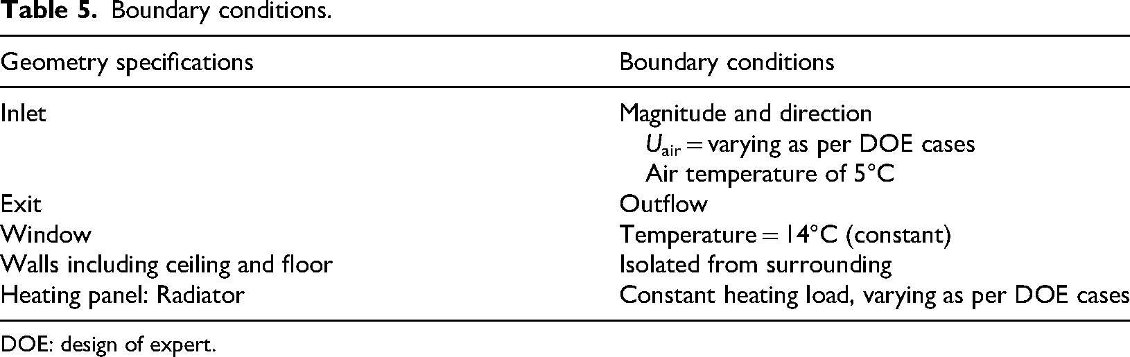
DOE: design of expert.

Grid independence test

Before proceeding toward the actual numerical simulations, a grid independence test (GIT) was carried out to confirm that the numerical results did not depend on the grid size. Three geometries with different grid sizes were meshed, and numerical simulations were carried out to analyze the indoor operative temperature at four monitoring locations, as shown in Figure 2. The numerical models with coarse, medium, and finely meshed geometries (0.5, 1, and 1.5 million grid cells) were modeled and found no considerable variation in the operative temperature computed for these geometries. The minor variations in operative temperature can be seen for different grid-sized mesh which can be neglected. The operative temperature was found to show similar trends. The mesh quality considerably affects the computational cost, time, and accuracy of the computation. To ensure computational accuracy and lower the cost and time related to the numerical simulations, geometry with a medium-sized mesh (1 million grid cells) has been selected for further computational analysis.

Figure 2.

GIT at lengths (a) l₁, (b) l₂, (c) l₃, and (d) l₄ from the radiator. (a) l₁ = 0.6 m, (b) l₂ = 1.8 m, (c) l₃ = 3.0 m, and (d) l₄ = 4.2 m. GIT: grid independence test.

Validation

Indoor occupant comfort is greatly affected by the IAT and fluid flow patterns. Also, the validation of the numerical model with an experimental setup ensures the precision and efficacy of the numerical results. Therefore, the validation of the basic geometric model has been carried out for comfort temperature at different monitoring locations. To enhance the accuracy of the numerical model, two validations with experimental investigation by Olesen et al.⁵³ and numerical study by Horikiri et al.⁵⁴ have been carried out as shown in Figure 3. For experimental validation, the operative temperature at X = 1 m from the radiator has been plotted, and for numerical validation, comfort temperature at four different monitoring lines has been verified, as shown in the Figure 3.

Figure 3.

Experimental and numerical validation at lengths (a) l₁, (b) l₂, (c) l₃, (d) l₄ and (e) X = 1 m from the radiator. (a) l₁ = 0.6 m, (b) l₂ = 1.8 m, (c) l₃ = 3.0 m, (d) l₄ = 4.2 m, and (e) X = 1 m.

To verify the validated results, the root mean square error (RMSE) was calculated for comfort temperature. Figure 3(a) shows an RMSE of 0.2 °C, Figure 3(b) shows 0.32 °C, Figure 3(c) demonstrates an RMSE of 0.27 °C and Figure 3(d) indicates RMSE of 0.24 °C. The average RMSE for comfort temperature is 0.25 °C. The comparison shows a nonconformity of ±0.5 °C with an RMSE of 0.25 °C in ITC between the results obtained from experiments by Olesen et al.⁵³ and Horikiri et al.,⁵⁴ which can be considered acceptable for further analysis. After the acceptable validation outcomes, further simulations were carried out to analyze the different Box–Behnken designs and optimize IEQ and energy demand using RSM.

Optimization of IEQ and energy demand

The optimization of IEQ and building energy demand consists of multiple conflicting objectives. The different comfort parameters govern the indoor occupant comfort such as air and radiation temperature, air velocity, occupant activity level, external work done, and clothing factor. While to optimize the building energy, the radiator heat load required to maintain the acceptable IAT should be minimized with maximum comfort. The input parameters such as IDI, air velocity of the incoming cold air, and radiator temperature need to be maintained in the range of −80 to +80 (Figure 1(b)), 0.1‒2 m/s, and 300‒310 K as discussed in the previous sections. The dependent variables including operative temperature, air velocity, PMV, PPD, and vertical gradient of temperature need to be optimized as per the requirement. The objective functions of occupant comfort and building energy demand optimization are contradictory since comfort needs to be maximized while the energy demand needs to be minimized. The function of occupant comfort optimization involves several variables such as indoor operative temperature, air velocity, and PMV index.⁵⁵ Here, for an optimum solution, the operative temperature need to be maintained in the range of 20‒22°C. In optimization of V_indoor, its magnitude need to be controlled less than 0.1 m/s and should be minimized for mixed ventilated IEQ. The PMV needs to be kept neutral at 0 within the limiting values of −0.5 to +0.5. Similarly, the temperature gradient needs to be minimized and its magnitude should be less than 1.5°C. The radiator temperature needs to be kept minimum since the indoor energy is assumed to be conserved without any loss to the walls and outdoor environment to optimize the energy demand of the building. These multiple conflicting objectives can be collectively optimized as multi-objective functions using the RSM.⁵⁶ The constraints to optimize the given problem are shown in Table 3. The detailed optimization algorithm for IEQ and building energy demand is well illustrated in Figure 4.

Figure 4.

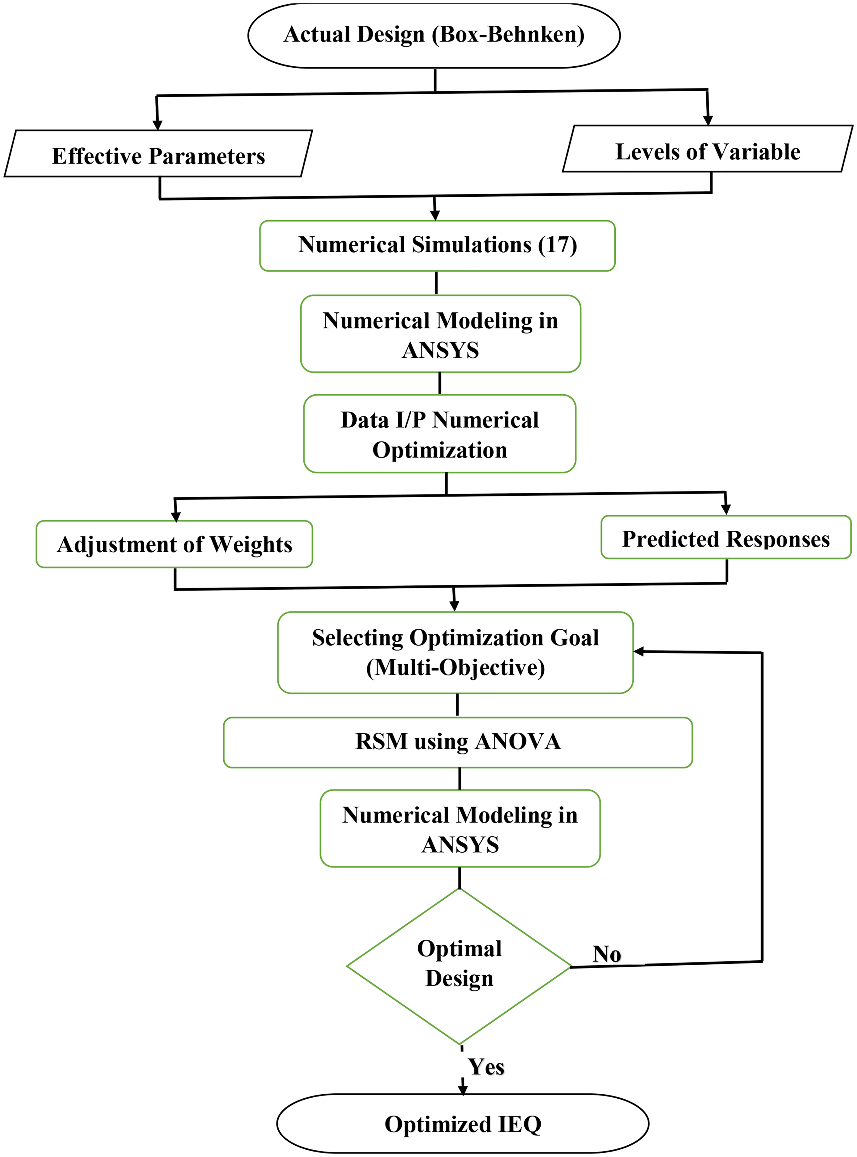
Optimization algorithm. ANOVA: analysis of variance; RMS: response surface methodology; and IEQ: indoor environmental quality.

Results and discussions

This segment deals with a thorough discussion of the effect of different independent variables on the response variables. After the generation of mesh, the successful grid independence test was performed, along with the validation of the numerical results with previously published experimental and numerical results. After the successful validation of the results, further methods have been followed as discussed in the previous sections. After the generation of the Box–Behnken design model, the necessary numerical analyses were carried out. The application of ANOVA gives different results, which can be further, and the optimized solution can be obtained. This section consists of the results about operative temperature, indoor air velocity, and PMV within a detailed discussion of the model fit summary, ANOVA analysis, diagnostics and 2-D and 3D model graphs in the subsequent sections.

This section deals with a detailed discussion of the combined outcome of various independent factors on the response variables. A successful mesh independence test was performed along with validation of the numerical outcomes with previously published experimental and numerical results after mesh generation. After the generation of the Box–Behnken design model, the necessary numerical simulations were performed using ANSYS Fluent 2023 R1. The application of ANOVA gives different results that can be further analyzed to obtain the optimized solution. This section consists of the results regarding the operative temperature, indoor air velocity, PMV index, and optimized solution with a detailed explanation of the model summary, ANOVA analysis, diagnostics, and 2D and 3D response surface plots in the following sections.

Operative temperature

It is a crucial parameter in assessing indoor comfort and fluid flow.⁵⁷ The influence of independent variables was identified on the response variables using ANOVA. It was found that the operative temperature is the best fit by a quadratic model with a highly significant value (P < .05). All variability in the data can be explained with 0.998 of R². The linear fit model was also significant with p-values <.007 and 0.704 R². The linear fit model shows simplicity with reasonable explanatory power, but the quadratic model was identified as the best fit model (Table 6). Although the two-factor interaction (2FI) model shows a reasonable R² value of .708, it is not significant since the p > .05. The signal-to-noise ratio (S/N) was found to be 86.246 (>4) which indicates that it can be used to navigate the design space. The outcomes signify that the operative temperature and independent variables exhibit a quadratic relationship that influences indoor occupant comfort.⁵⁵

Table 6.

Operative temperature fit statistics.

Standard Deviation	0.1007	R²	0.9998
Mean	292.29	Adjusted R²	0.9984
C.V. %	0.0345	Predicted R²	1
		S/N ratio	86.2457

The value of 0.0014 obtained from the ANOVA analysis indicates a higher model significance, in which that the independent variables strongly influence the response variables. The F-value of 712.22 as shown in Table 7, suggests that the model is statistically significant, with only a 0.14% probability that such a large F-value could arise from random variation. The lowest p-value of the radiator temperature indicated that the operative temperature is most significantly influenced by the radiator temperature,⁵⁸ followed by inlet air velocity and IDI with p-values of .0003, .0008, and .0012 correspondingly with a linear relationship. The IDI exhibits a non-linear quadratic effect on the operative temperature with a significant p-value of .0026. The interaction between the inlet air velocity and radiator temperature affects the operative temperature considerably, so the interaction between these independent variables plays an important role in shaping the operative temperature. This indicates that the combined and individual impacts of the independent variables are crucial in optimizing the operative temperature.

The equations, in actual terms, are predictive tools for estimating operative temperature at specified input levels. Due to the scaling of coefficients and the offset intercept, they should not be utilized to determine the relative influence of each factor. Four levels of air velocity have been selected to investigate the influence of the independent variables on the operative temperature. The following equations were formulated to forecast the operative temperature response at four different levels of velocity magnitude, 0.1, 1, 1.5, and 2 respectively as shown in equations (23)–(26). The response at other velocity points can be predicted by interpolation or by fitting the general equations. The 3D response surface plots for the operative temperature at 0.1, 1, 1.5, and 2 m/s can be plotted as shown in Figure 5(a)–(d) correspondingly based on the equations:

T_{o p e r a t i v e} = 1502.82 + 0.56 A - 9.43 C - 0.0018 A C + 0.00084 A^{2} + 0.017 C^{2}

(23)

T_{o p e r a t i v e} = 1843.83 + 0.55 A - 10.56 C - 0.0018 A C + 0.00084 A^{2} + 0.017 C^{2}

(24)

T_{o p e r a t i v e} = 1864.26 + 0.56 A - 10.63 C - 0.0018 A C + 0.00084 A^{2} + 0.017 C^{2}

(25)

T_{o p e r a t i v e} = 1789.71 + 0.55 A - 10.39 C - 0.0018 A C + 0.00084 A^{2} + 0.017 C^{2}

(26)

Figure 5.

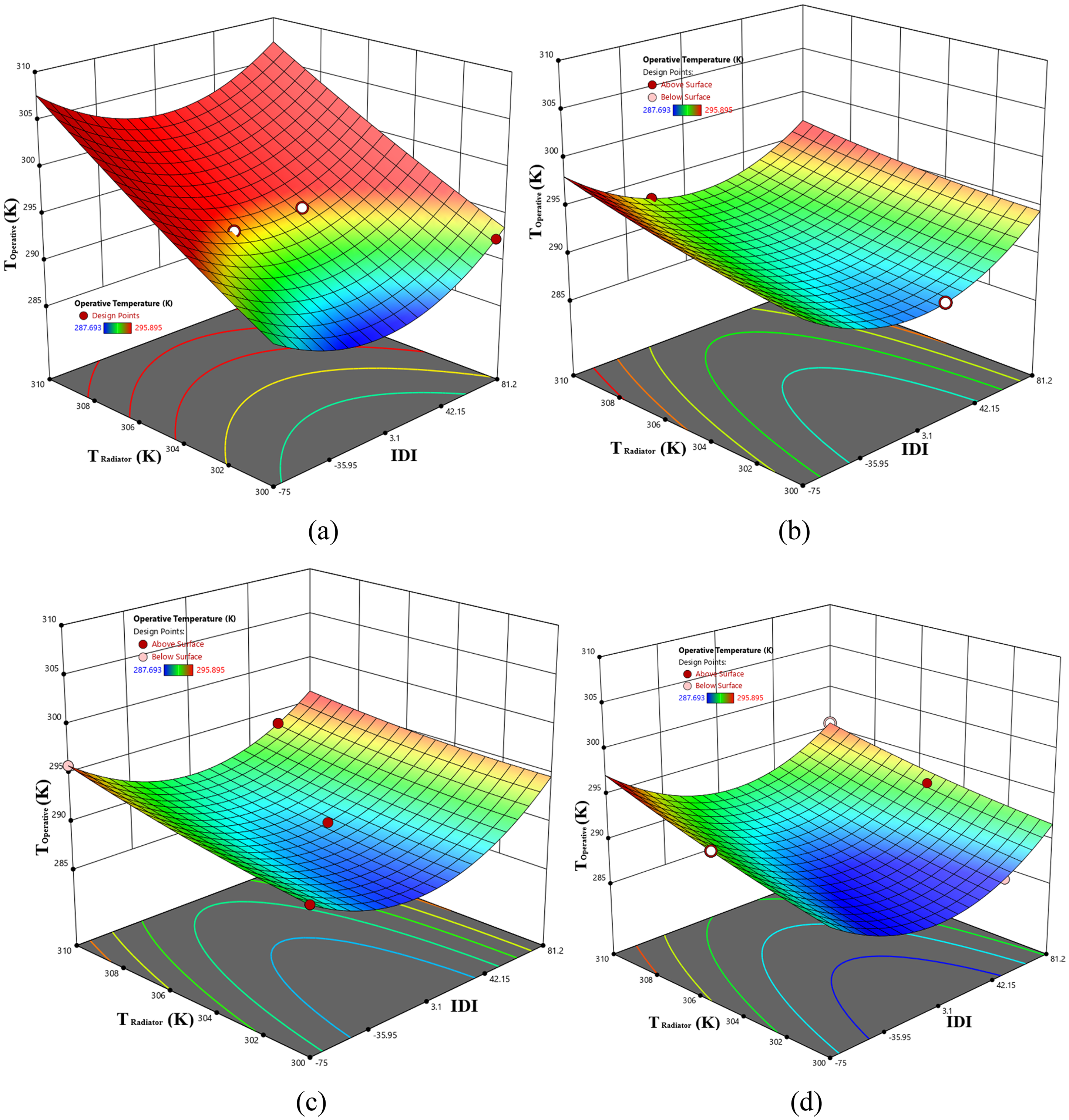
3D response surface plot for operative temperature at (a) 0.1 m/s, (b) 1 m/s, (c) 1.5 m/s, and (d) 2 m/s.

Figure 5 shows the Box–Behnken design points with the optimal solution indicated by white dots and red dots. At 0.1 m/s of air velocity, the optimal operative temperature can be obtained by keeping the IDI at 75° and the radiator temperature at 300 K. The operative temperature of the indoor air was obtained as 293.72 K independent of the other variable settings, which is within the acceptable range of indoor comfort temperatures. At lower speeds, the acceptable operative temperature can be lowered to a lower radiator heat load for a wide range of IDI. When the outlet air speed is increased to 1 m/s, the design changes to −22.8° IDI with a radiator temperature of 310 K, which gives an operative temperature of 293.186 K. The operative temperature for IDI near the normal-to-boundary region results in a lower operative temperature. For these IDIs even at the higher radiator temperatures, the design fails to maintain an acceptable indoor operative temperature which indicates the impact of multiple factors on the indoor operative temperature. As the IDI increases to the extreme boundary conditions, the operative temperature can be improved at lower radiator temperatures. For a ventilation velocity of 1.5 m/s, the optimal design IDI point can be set at 58.4° IDI and a radiator temperature of 310 K, which needs further optimization for indoor comfort and energy demand. The optimal solution region contracts, and no design points satisfy the acceptable operative temperature for a velocity of 2 m/s at elevated air velocities such as 1.5 and 2 m/s.

Figure 6 shows the 2D response contour plot for operative temperature at different inlet air velocities. The contour area shaded in blue color shows the region of the independent variable combinations, resulting in unacceptable operative temperatures. The region in red represents the optimal design values of the independent variables. Similar design points can be observed in the 3-D contour plots for optimal solutions.

Figure 6.

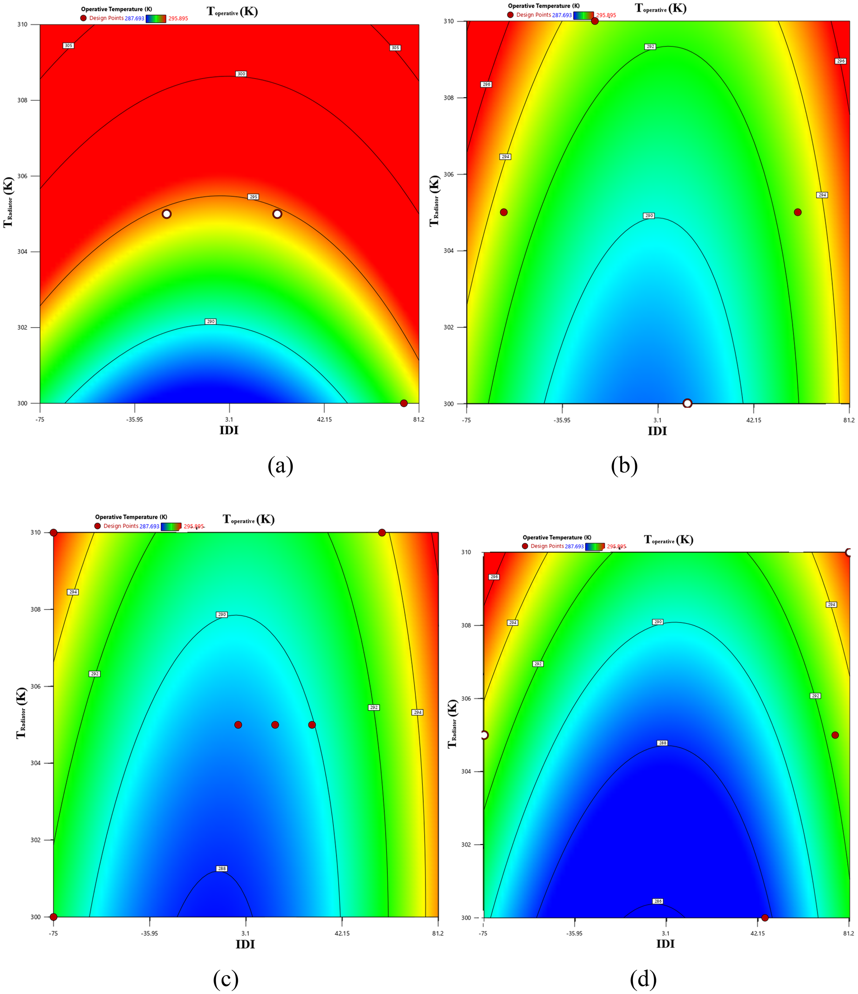
2D response contour plot for operative temperature at (a) 0.1 m/s, (b) 1 m/s, (c) 1.5 m/s, and (d) 2 m/s. IDI: inlet diffuser inclination.

Indoor air velocity

In high-volume buildings, indoor air velocity is influenced by indoor/outdoor temperature and pressure variations, but in the case of small buildings, the indoor air velocity is influenced by the IAT mainly.⁵⁷ Inadequate indoor air movement affects indoor occupant comfort due to excess eddies and circulation in the indoor environment which causes occupant discomfort due to the sensation of drafts and cold airflows.⁵⁹ In this section, efforts are taken to evaluate the effect of different independent variables on indoor air movement by using ANOVA. It was found that the indoor air velocity function is best described by the 2FI model with a highly significant value of P-value < 0.0035. The inconsistency in the analyzed and predicted values can be clarified with a 0.9869 value of R². The S/N ratio was found to be 15.70 (>4) which indicates that this model can be used to navigate the indoor air velocity for design space. The outcomes as shown in Table 8 signify that the indoor air velocity and the independent variables exhibit a 2FI relationship which influences indoor comfort. Table 9 shows that indoor air velocity depends on two factors, IDI and V_inlet, and is independent of the radiator temperature. This supports the suitability of the 2FI model for the fit summary.

Table 7.

ANOVA for operative temperature.

Variables	Sum of squares	df	Mean square	F-value	p-value
Model	101.16	14	7.23	712.22	.0014
A: IDI	8.81	1	8.81	867.96	.0012
B: V_inlet	37.64	3	12.55	1236.78	.0008
C: T_Radiator	29.90	1	29.90	2947.58	.0003
A²	3.87	1	3.87	381.85	.0026
BC	1.56	3	0.5197	51.22	.0192

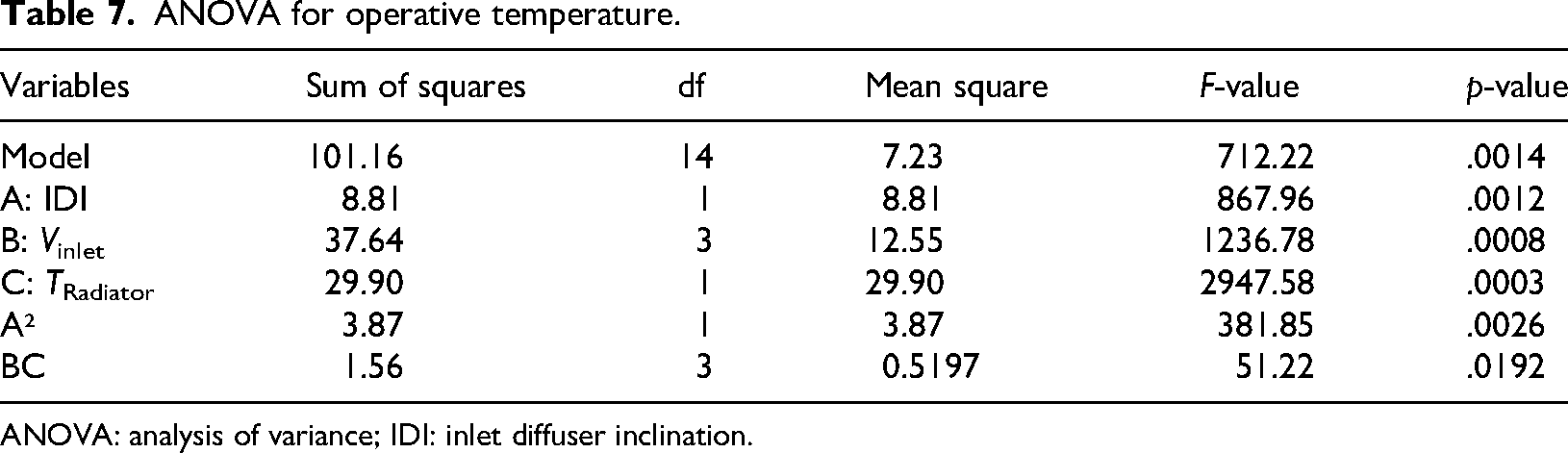
ANOVA: analysis of variance; IDI: inlet diffuser inclination.

Table 8.

Indoor air velocity fit data.

Standard deviation	0.0031	R²	.9869
Mean	0.0580	Adjusted R²	.9476
C.V. %	5.38	Predicted R²	1.00
		S/N ratio	15.7078

Table 9.

ANOVA for indoor air velocity.

Source	Sum of squares	df	Mean square	F-value	p-value
Model	0.0029	12	0.0002	25.11	0.0034
A: IDI	0.0011	1	0.0011	115.78	0.0004
B: V_inlet	0.0011	3	0.0004	36.66	0.0023
AB	0.0003	3	0.0001	10.59	0.0226
AC	0.0001	1	0.0001	10.76	0.0305

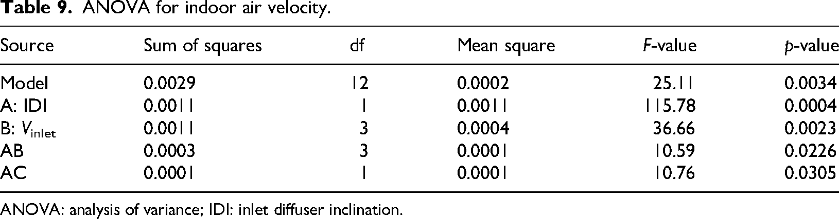
ANOVA: analysis of variance; IDI: inlet diffuser inclination.

The P-value of .0034 obtained from the ANOVA analysis indicates the impact of the model which signifies the influence of independent variables on the indoor air velocity. The model F-value of 25.11 indicates that the model is important and a 0.34% chance that such a large F-value could occur due to noise.

The lowest p-value of the IDI indicated that the velocity is most significantly influenced by the IDI followed by inlet air velocity with p-values of .0004 and .0023, respectively, with a linear relationship. There is no non-linear quadratic effect of independent variables on the velocity. The interaction between the IDI and inlet air velocity affects the velocity considerably. Additionally, the interaction between IDI and radiator temperature combinedly affects the velocity, so the interplay between these independent variables plays an important role in manipulating the indoor air velocity. This indicates that the combined and individual impacts of independent variables are crucial in optimizing the operative temperature. The equations shown below in equations (27)–(30), in actual terms, are predictive tools for estimating indoor air velocity at specified input levels.

V_{i n d o o r} = - 0.99 + 0.0068 A + 0.0034 C - 2.25 e - 05 A C

(27)

V_{i n d o o r} = - 0.36 + 0.0069 A + 0.0013 C - 2.25 e - 05 A C

(28)

V_{i n d o o r} = 0.11 + 0.0071 A - 0.00015 C - 2.25 e - 05 A C

(29)

V_{i n d o o r} = 0.313 + 0.0070 A - 0.00083 C - 2.25 e - 05 A C

(30)

To analyze the influence of the independent variables on indoor air velocity, 4 levels of air velocity have been selected. The following equations can be formulated to forecast the operative temperature response at four altered levels of the velocity magnitudes, 0.1, 1, 1.5, and 2 m/s, respectively, as shown in equations (27)–(30). The response at other velocity points can be predicted by interpolation or by fitting the general equations. Based on the equations, the 3-D response surface plots for the indoor air velocity at the respective inlet velocities can be plotted in Figure 7(a)–(d), respectively. The optimal solutions as per the Box–Behnken design can be observed at −22.8 and +22.8 IDI with a radiator temperature of 305 K at an inlet velocity of 0.1 m/s. For an elevated velocity of 1 m/s, the design points with the setting of IDI of 15 and 300 K of radiator temperature result in velocity of 0.05 m/s, which is acceptable for indoor occupant comfort under the constraint conditions. A further rise in inlet air velocity shifts the optimal solution points toward higher radiator temperatures and the absolute values of IDI. As inlet velocity rises to 1.5 and 2 m/s, the IDI of 58.2 and 45 along with the higher radiator temperatures of 300‒310 K, respectively, gives the optimal outcomes. This shows that higher inlet air velocity requires advanced absolute IDI and lower radiator temperatures to maintain the indoor operative temperature within acceptable limits. This is because the inlet air makes direct contact with the radiator before it is mixed with the indoor air, which increases the velocity because of the obvious buoyancy effect. The 3D surface plot shows that as the inlet air velocity increases and IDI advances beyond the absolute normal boundary direction, the indoor air velocity also increases regardless of the radiator temperature. This shows that high inlet air velocity with improper IDI alignment substantially increases indoor air velocity, causing discomfort to occupants by creating cold drafts, eddies, and circulations in the region. Figure 8 shows the 2D response contour plot of velocity at altered inlet air velocities. The contour area shaded in blue shows regions of the independent variable arrangement, giving an acceptable indoor air velocity. The region in red represents the higher indoor air velocity which causes the indoor occupant discomfort, and the design points correspond to those discussed in the 3D surface plots. As the inlet air velocity increases in the subsequent cases, the blue region keeps on contracting and becomes minimum for 2 m/s velocity which represents that the indoor air velocity further increases with an increase in inlet air velocity.

Figure 7.

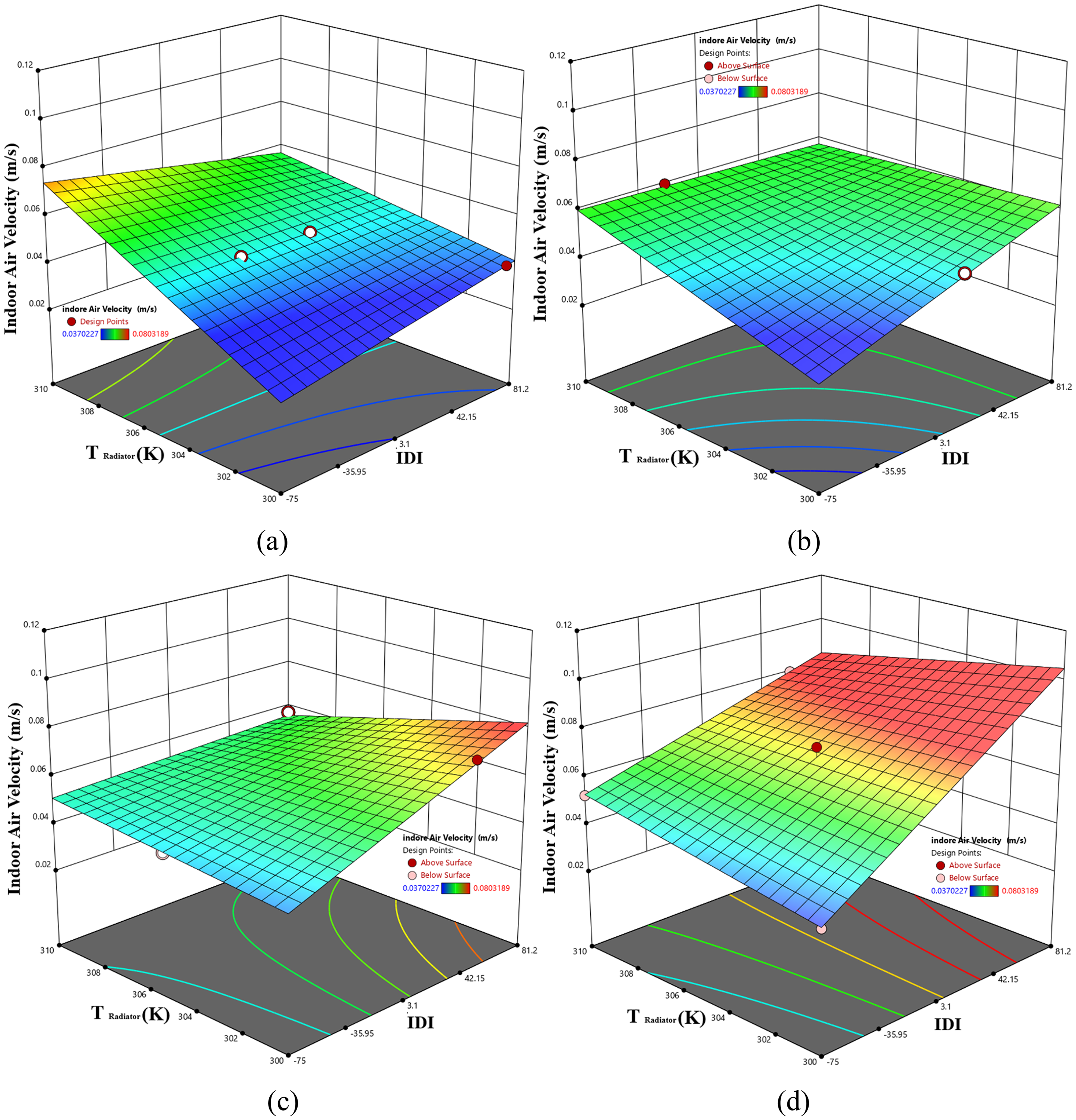
3D response surface plot for indoor air velocity at (a) 0.1 m/s, (b) 1 m/s, (c) 1.5 m/s, and (d) 2 m/s. IDI: inlet diffuser inclination.

Figure 8.

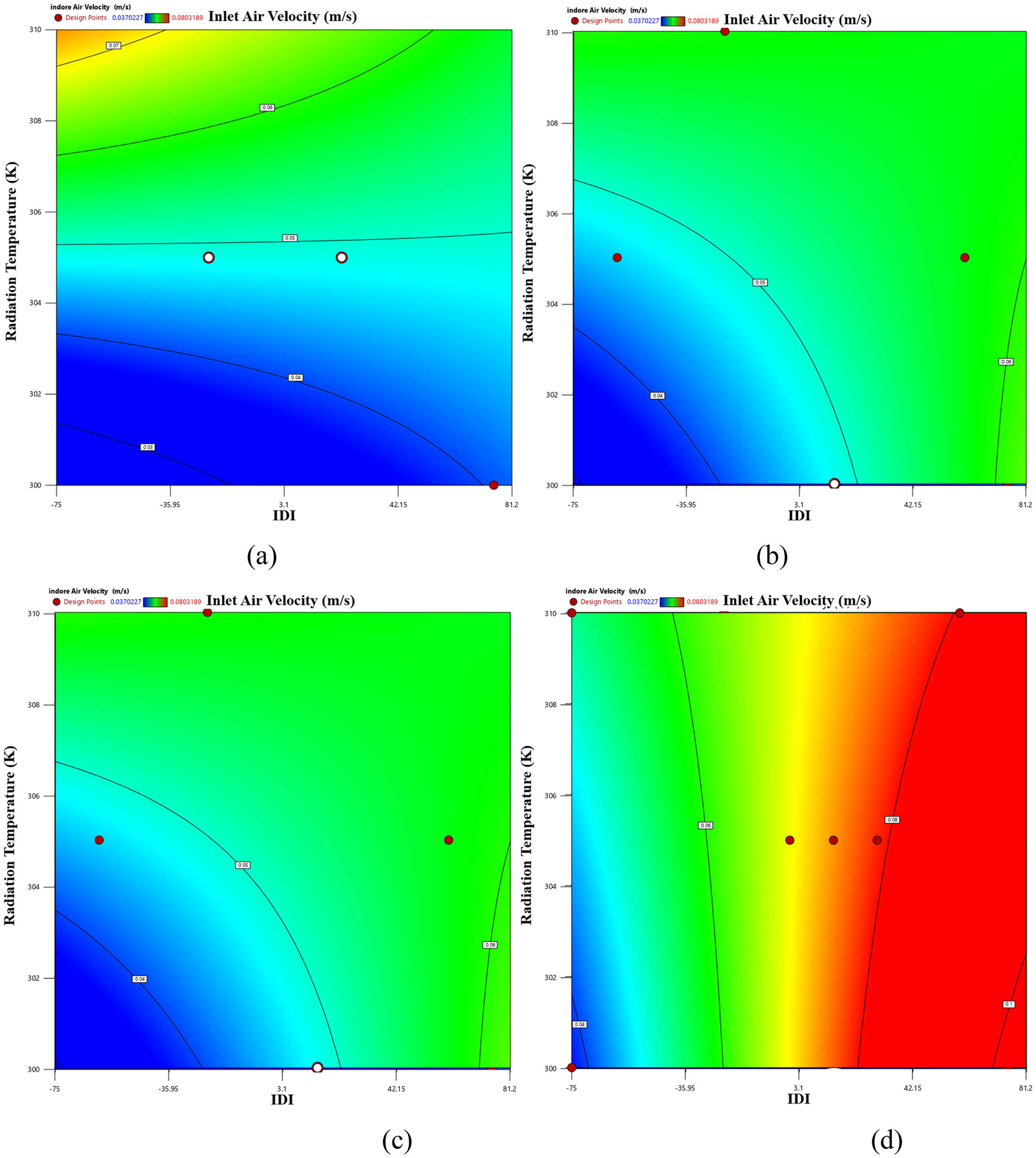
2D response contour plot for indoor air velocity at (a) 0.1 m/s, (b) 1 m/s, (c) 1.5 m/s, and (d) 2 m/s. IDI: inlet diffuser inclination.

Figure 8 shows that increasing the absolute IDI inclination angle can help reduce the effect of high inlet air velocity. This adjustment creates design points where the building parameters or independent variables can be optimized to achieve lower indoor air velocity even at elevated inlet air velocities. However, as the inlet velocity increases, this favorable region decreases and moves towards higher IDI values.

Additionally, increasing the radiator temperature has minimal effect on indoor air velocity, indicating that radiator temperature is not a significant factor affecting indoor air velocity. The IDI remains a critical factor in effectively controlling indoor air velocity.

PMV

PMV, AMV, and PPD are the historical models used to identify indoor occupant comfort. These are the most widely used models, while the PPD model is dependent on PMV; hence, it was preferred to analyze the PMV, which determines the indoor comfort.^48,49 In this section, efforts have been made to find the effect of different independent variables on the PMV index using ANOVA.

It was found that the PMV index is best described by a quadratic relation model with a highly significant P <.0011. The inconsistency in the analyzed and predicted standards can be described with an R² of .99 value. The S/N ratio was found to be 28.98 (>4) which indicates that this model can be used to navigate the PMV index for indoor comfort and energy demand design space. The linear fit model shows simplicity with reasonable explanatory power, but the quadratic model was recognised as the best appropriate model fit (Table 10).

Table 10.

PMV fit statistics.

SD	0.0551	R²	.9984
Mean	−0.3824	Adjusted R²	.9874
C.V. %	14.41	Predicted R²	1
		S/N ratio	28.9862

PMV: predicted mean vote.

The outcomes signify that the operative temperature and independent variables exhibit a quadratic relationship that influences indoor occupant comfort.⁵⁷ Table 11 shows that the PMV index depends on all three factors, IDI, V_inlet, and T_radiator. This supports the suitability of the quadratic fit model for the fit summary. The acceptable p-values indicated that the PMV index is most significantly affected by the radiator temperature followed by inlet air velocity and IDI with p-values of .0031, .0058, and .0111, respectively, with a quadratic relationship. The IDI exhibits a non-linear quadratic effect on the operative temperature, with a significant p-value of .0259.

P M V = - 220.55 - 0.11 A + 1.19 C + 0.00039 A C + 0.00014 A^{2} - 0.0015 C^{2}

(31)

P M V = - 168.74 - 0.12 A + 1.018 C + 0.00039 A C + 0.00014 A^{2} - 0.0015 C^{2}

(32)

P M V = - 171.13 - 0.12 A + 1.02 C + 0.00039 A C + 0.00014 A^{2} - 0.0015 C^{2}

(33)

P M V = - 163.39 - 0.12 A + 0.99 C + 0.00039 A C + 0.00014 A^{2} - 0.0015 C^{2}

(34)

Table 11.

ANOVA for PMV.

Variables	Sum of squares	df	Mean square	F-value	p-value
Model	3.84	14	0.2742	90.34	.0011
A: IDI	0.2678	1	0.2678	88.24	.0111
B: V_inlet	1.55	3	0.5166	170.23	.0058
C: T_Radiator	0.9758	1	0.9758	321.52	.0031
A²	0.1127	1	0.1127	37.13	.0259

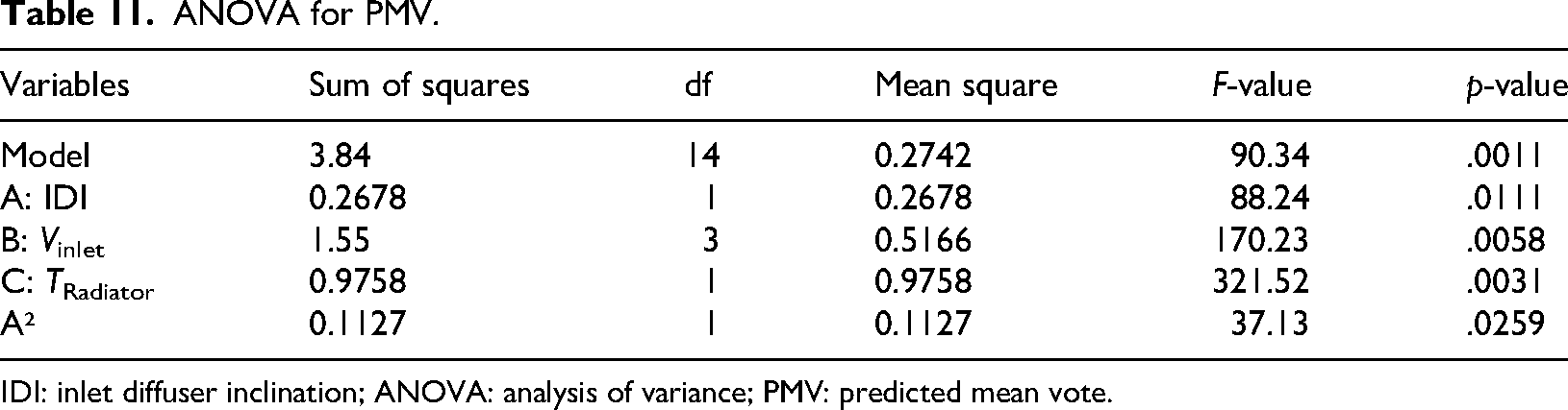
IDI: inlet diffuser inclination; ANOVA: analysis of variance; PMV: predicted mean vote.

The equations, in actual terms, are predictive tools for estimating operative temperature at specified input levels. To analyze the effect of the independent variables on the PMV index, 4 levels of the inlet air velocity were selected. Equations (31)–(34) can be formulated to forecast the operative temperature response at four altered velocity magnitude levels, 0.1, 1, 1.5, and 2 m/s, respectively, as shown in equations (31)–(34). The response at other velocity points can be predicted by interpolation or by fitting the general equations. Based on the equations, the 3D response surface plots for the PMV index at different inlet air velocities can be plotted as Figure 9(a)–(d) respectively. For 0.1 m/s, inlet velocity the optimal PMV index can be obtained by keeping IDI at 75° and radiator temperature at 300 K, as per the cases generated by the Box–Behnken design. The PMV index obtained at this point is −0.3 which is in the acceptable range. The blue shaded area shows the independent design variable region where the PMV index is lower than the required comfort standards. As the inlet air velocity increases, the red region which shows the favorable design area contracts and the blue shaded area increases which signifies that, the PMV index is more difficult to maintain within an acceptable range at higher velocities. At higher inlet air velocities, higher temperature is required to maintain the PMV index in an acceptable range.

Figure 9.

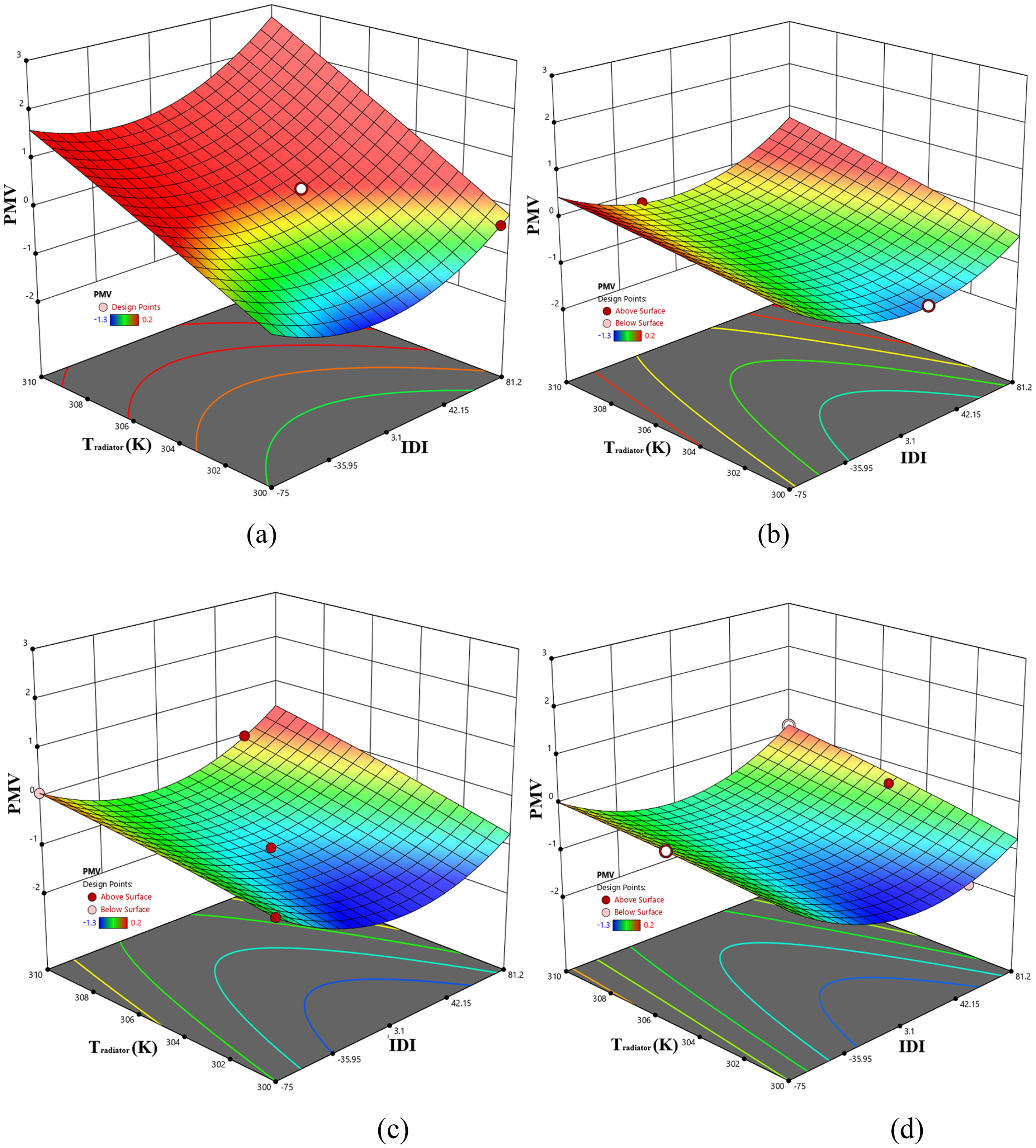
3D response surface plot for indoor air velocity at (a) 0.1 m/s, (b) 1 m/s, (c) 1.5 m/s, and (d) 2 m/s. IDI: inlet diffuser inclination.

Figure 10 shows the 2D response contour plot for the PMV index at different inlet air velocities. The contour area shaded in blue shows the region of the independent variable combination, giving an unacceptable PMV index. The region in red represents the optimal design values required of the independent variables. Similar design points can be observed from the 3D contour plots for optimal solutions. As the inlet air velocity increases, the blue-shaded area increases in the region of normal-to-boundary IDI, while increasing the IDI optimizes the PMV index in an acceptable range.

Figure 10.

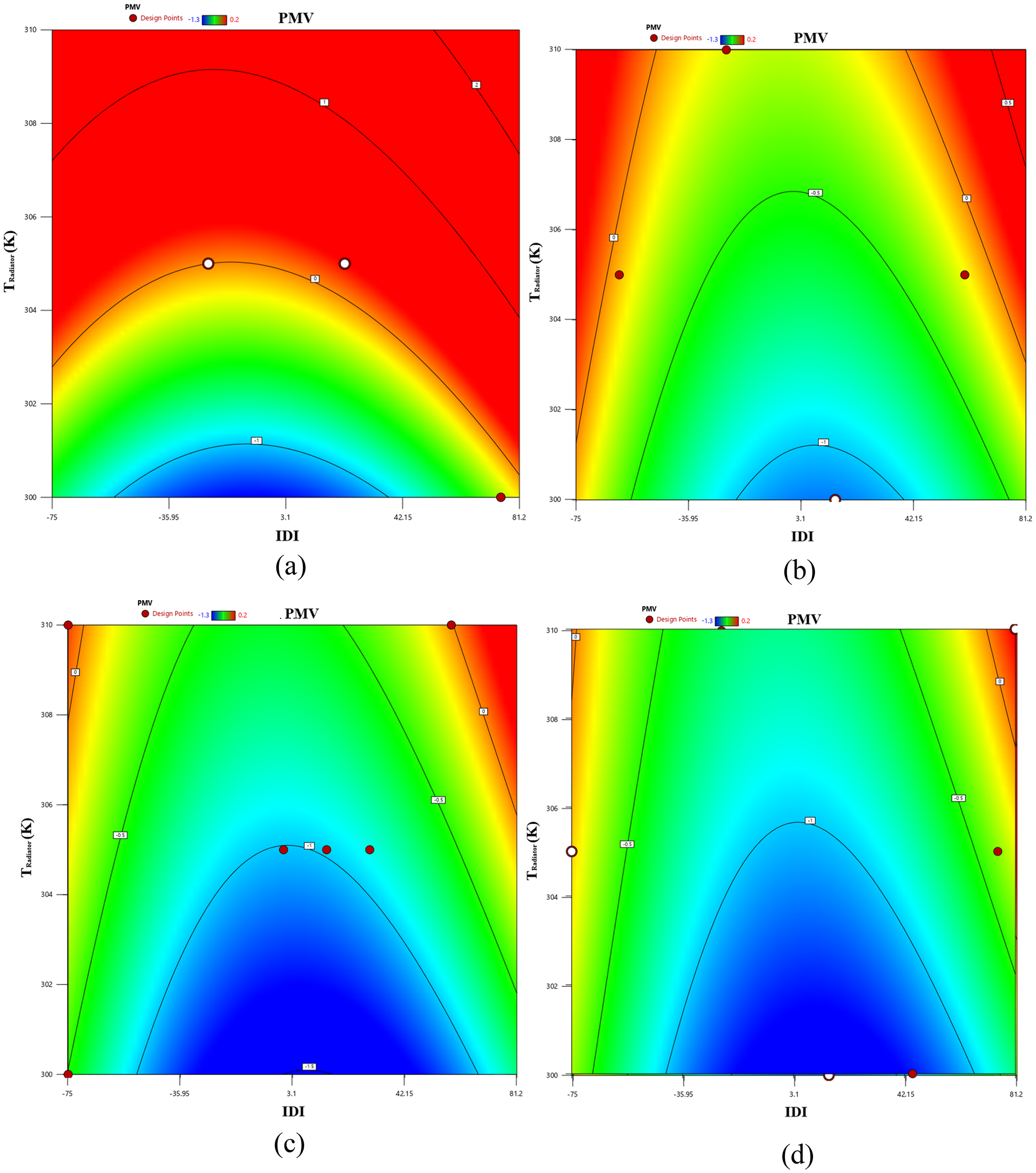
2D response contour plot for indoor air velocity at (a) 0.1 m/s, (b) 1 m/s, (c) 1.5 m/s, and (d) 2 m/s. IDI: inlet diffuser inclination.

A high IDI enhances occupant comfort (PMV index) even at high inlet air velocities, effectively addressing potential draft issues in occupied areas. The high IDI angles direct inlet cold air towards strategic locations such as radiators or ceilings by improving airflow patterns.⁶⁰ This is important because buoyancy causes warm air to rise and accumulate near the ceiling. Directing cold inlet air near the ceiling and radiator leads to better mixing of warm and cold air, ensuring that mixing occurs away from occupied zones. This balanced intermixing helps achieve a more acceptable and evenly regulated indoor environment. This signifies that the higher IDI can control the comfort of indoor occupants even at elevated inlet air velocities, even though the elevated velocity in the region near the occupant can create the draft problems.

Optimization of the model for IEQ

The optimal solution for the defined constraints is shown in Table 12. To optimize the room model, efforts have been taken to retain the indoor operative temperature of 20–23°C and velocity less than 0.1 m/s with a PMV index within the acceptable limit of −0.5 to +0.5, which meets the cold climate limiting indoor comfort requirements. The objective function can be manipulated as per the requirement of the indoor occupants and building design requirements by changing the constraints and conditions. The RSM suggests an optimized statistical solution with IDI set at −76.52 through an inlet air velocity of 0.1 m/s and T_radiator at 300 K. For the similar boundary conditions for the independent variables, a detailed analysis of the IEQ was carried out numerically. Table 12 shows a comparison between statistical and numerical methods to accurately identify the accuracy of the statistical method (RMSE) with a numerical method. The numerical results of the response variables according to the statistical optimization show tolerable agreement with the numerical results with RMSE of 0.228, 0.002, and 0.022 for radiator temperature, indoor air velocity, and PMV index, respectively. The mean RMSE between the statistical and numerical values in the verification experiment was 4.73%.

Table 12.

Optimized independent variables.

Method	IDI	V _inlet	T _radiator	T _operative	V _indoor	PMV	Desirability
Statistical	−76.52	0.1	300	293.102	0.041	−0.238	1.000
Numerical	−76.52	0.1	300	293.33	0.043	−0.216	—
RMSE	0.228	0.002	0.022

RMSE: root mean square error; PMV: predicted mean vote; IDI: inlet diffuser inclination.

After simulating the statistical design with the numerical method using CFD, comfort parameters were compared for temperature, temperature gradient, IAT, indoor air vector, indoor air velocity, and PMV index as per the occupant comfort requirement of the occupants under cold climatic conditions. The operative temperature has been monitored at four different locations as shown in Figure 1 monitoring lines. Figure 11(a) shows the operative temperature trends at four different monitoring lines. At all four locations, the IAT was found to be higher than the limiting condition for indoor comfort. The operative temperature in the indoor environment at all the locations was found to be uniform throughout the height of the room and higher than 293 K, which is the limiting condition for occupant comfort.¹² Slight variations in operative temperature near the radiator can be seen due to the existence of higher buoyancy forces. The mixing zone is generally exposed to the radiator surface and due to the intensity of radiation in the adjacent regions, higher temperatures are observed in these regions, while above the radiator surface, the operative temperature shows a more uniform distribution⁶¹ Figure 11(b), shows the IAT contour to analyze the overall temperature distribution of the indoor fluid domain.

Figure 11.

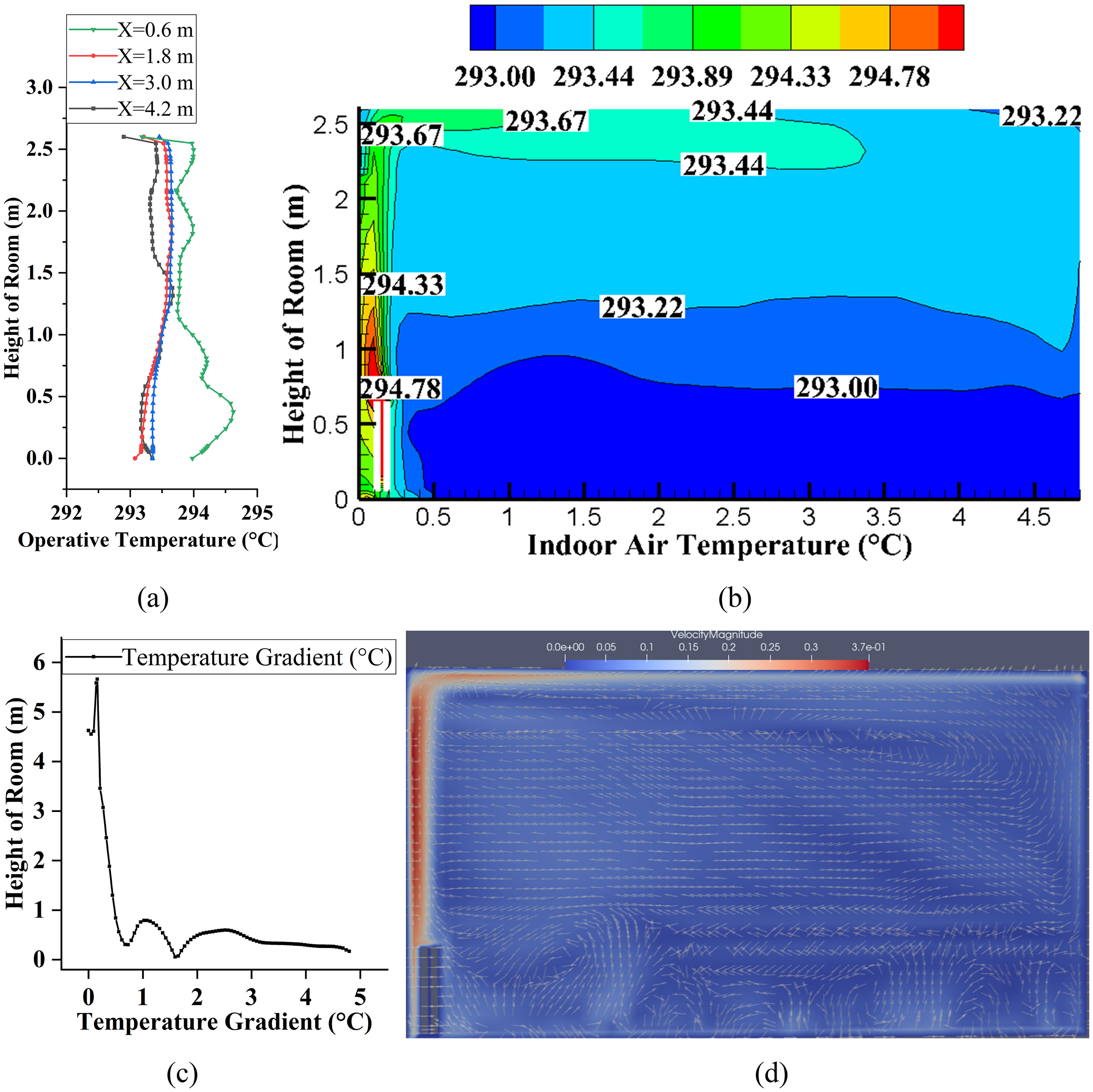
(a) Operative temperature, (b) 2D contour plots of IAT, (c) temperature gradient, and (d) 2D contour plots of the velocity vector. IAT: indoor air temperature.

The stable stratification layers exhibit a uniform thermal IAT within an acceptable range. Lower temperatures can be observed at the ground level; in the fluid domain above the ground, the IAT gradually increases due to the buoyancy effect. Near the window and under the input diffuser, temperatures are higher than they are above the radiator. This area is commonly known as the mixing zone where the mixing of cold air and hot air occurs by the buoyancy effect.⁶² This area should be as small as possible to maximize the occupied space available to the occupants.

The indoor temperature gradient must be smaller than 1.5°C, representing the temperature difference between the ankle and neck levels of occupants. The indoor occupant is assumed to be standing indoors to analyze this comfort parameter. Figure 11(c) shows the temperature gradient for the optimized design solution for the building design. The temperature gradient close to the radiator and inlet vent was found to be higher compared to the gradient in the region 0.6 m away from the radiator.⁶³ Despite the elevated temperature differential in the mixing zone, the temperature gradient in the occupied area was determined to be below 1°C. Indoor air movement plays a crucial role in determining comfort levels, as it influences occupant comfort through the intensity of eddies and circulation, which can lead to cold draft issues. Figure 11(d) shows the velocity vector contour for the optimized numerical model suggested by the statistical model. Indoor velocity was restricted to 0.1 m/s in most of the regions, while higher velocity can be observed in the mixing zone. Also, considerable eddies and circulation can be seen near the floor region as a result of the buoyancy effect and surface boundary layers. The region near the walls shows the higher circulation of cold air but the lower magnitude of air velocity avoids the risk of cold draft problems. The PMV index calculated from the numerical solution was found to be close to the statistical solution with an RMSE of 0.022. The PMV index shows a slightly colder indoor environment but in the range of indoor comfort requirements as per the standards. To optimize the PMV index to a neutral value, the necessary changes can be made in the objective function constraints during the statistical method of optimization.

The findings derived from the RSM closely align with the numerical results, effectively meeting all comfort requirements while using the least energy necessary for the radiator. This approach minimizes the building energy consumption needed to maintain indoor comfort. It is possible to attain an optimal balance among indoor comfort and energy demand through multi-objective function optimization by integrating statistical and numerical methods.⁶⁴

Conclusions

This study employs a novel approach that combines statistical methods (RSM) with numerical methods (CFD) to determine the optimal IEQ for a comfort parameter design, aiming to attain the utmost indoor comfort with minimizing the building energy demand. The methodology aims to establish an appropriate balance between acceptable IEQ and energy efficiency. Experimentally and numerically well-validated CFD models have been employed to analyze the accuracy of the statistical model and study the statistically optimized solution for IEQ and energy demand. The main outcomes drawn from the study are as follows.

The statistically optimized solution using RSM provides the best parameters as IDI = –76.52, inlet air velocity = 0.1 m/s, and radiator temperature = 300 K. The statistical outcomes align closely with numerical results with RMSE of 0.228 for 0.002, and 0.022 for radiator temperature, indoor air velocity, and PMV index. The mean RMSE in verification experiments was 4.73%, confirming the reliability of the model.

The T_operative for evaluating indoor comfort is effectively modeled through a quadratic relationship with independent variables and shows significant statistical relevance with a P-value < .003 with an exceptional R² of .998. Among the influencing factors, T_radiator is the most critical, followed by V_inlet and IDI.

V_indoor fits best with a 2FI model, as indicated by its high level of significance with a P-value < .0035 and strong predictive capability R² = .9869. The model also features IDI (P = .0004) as the most significant variable and inlet air velocity (P = .0023) as the least influential parameter for V_indoor while both following a linear trend without quadratic effects.

The PMV index is most accurately captured using a quadratic model with a highly significant P < .0011 as a statistical outcome. The radiator temperature with a P-value of .0031 is the primary influencing factor, followed by inlet air velocity with a P-value of .0058 and IDI with a P-value of .0111 with quadratic relationships. Furthermore, IDI shows a notable non-linear quadratic influence on T_operative with a P-value.

Performing all possible combinations of independent variables to confirm optimal results is often impractical and costly. The statistical methods applied in this study have proven highly effective for experimental, numerical, and analytical analyses. They hold significant potential for modeling indoor environments while addressing ventilation, air quality, thermal comfort, and energy efficiency.

Footnotes

Author Note

Ghogare Abhijeet Ganesh are now affiliated with MAEER’s Maharashtra Institute of Technology, Thane, Mumbai, India.

ORCID iD

Tikendra Nath Verma

Authors’ contribution

Abhijeet Ganesh Ghogare contributed to software, investigation, methodology, and writing–original draft. Shobha Lata Sinha contributed to conceptualization, validation, visualization, and supervision. Vijay Panchore contributed to formal analysis, resources, and data curation. Tikendra Nath Verma contributed to formal analysis, resources, and writing–review & editing.

Funding

The authors received no financial support for the research, authorship, and/or publication of this article.

Declaration of conflicting interests

The authors declared no potential conflicts of interest with respect to the research, authorship, and/or publication of this article.

References

Yang

Yan

Lam

. Thermal comfort and building energy consumption implications – A review. Appl Energy 2014; 115: 164–173.

I.E. Agency . Transition to sustainable buildings: strategies and opportunities to 2050. Paris: IEA Publ, 2013.

Birol

. The future of cooling. Tech. rep, IEA, 2018. https://www.iea.org/reports/the-future-of-cooling .

Dimitroulopoulou

Dudzińska

Gunnarsen

, et al. Indoor air quality guidelines from across the world: an appraisal considering energy saving, health, productivity, and comfort. Environ Int 2023; 178: 108127.

Schulze

Eicker

. Controlled natural ventilation for energy efficient buildings. Energy Build 2012; 56: 221–232.

Stasi

Ruggiero

Berardi

. Influence of cross-ventilation cooling potential on thermal comfort in high-rise buildings in a hot and humid climate. Build Environ 2024; 248: 111096.

Tong

Chen

Malkawi

, et al. Energy saving potential of natural ventilation in China: the impact of ambient air pollution. Appl Energy 2016; 179: 660–668.

Oropeza-Perez

Østergaard

. Energy saving potential of utilizing natural ventilation under warm conditions – A case study of Mexico. Appl Energy 2014; 130: 20–32.

Peng

Lei

Tekler

, et al. Hybrid system controls of natural ventilation and HVAC in mixed-mode buildings: a comprehensive review. Energy Build 2022; 276: 112509.

10.

Deuble

De Dear

. Mixed-mode buildings: a double standard in occupants’ comfort expectations. Build Environ 2012; 54: 53–60.

11.

Sakiyama

Carlo

Frick

, et al. Perspectives of naturally ventilated buildings: a review. Renewable Sustainable Energy Rev 2020; 130: 109933.

12.

ASHRAE. 10P Guideline, Interactions Affecting the Achievement of Acceptable Indoor Environments, ASHRAE, Atlanta, USA, 2010. Second Public Review

13.

Brager

. Mixed-mode cooling. ASHRAE J 2006; 48: 30.

14.

Ganesh

Sinha

Verma

, et al. Investigation of indoor environment quality and factors affecting human comfort: a critical review. Build Environ 2021; 204: 108146.

15.

Frontczak

Andersen

Wargocki

. Questionnaire survey on factors influencing comfort with indoor environmental quality in Danish housing. Build Environ 2012; 50: 56–64.

16.

Gao

Wang

Zhang

, et al. Numerical investigation on the relationship between human thermal comfort and thermal balance under the radiant cooling system. Energy Proc 2017; 105: 2879–2884. https://10.1016/j.egypro.2017.03.640

17.

Ahmed

Gao

. Thermal comfort and energy-saving evaluation of a combined system in an office room using displacement ventilation. Int J Mech Aerosp Ind Mech Manuf Eng 2015; 44: 1085–1090. https://10.5281/zenodo.1107603

18.

Zhangping

Chuanping

, et al. Effect of natural ventilation on indoor air quality and thermal comfort in dormitory during winter. Build Environ 2017; 125: 240–247. https://10.1016/j.buildenv.2017.08.051

19.

Federspiel

Fisk

Price

, et al. Worker performance and ventilation in a call center: analyses of work performance data for registered nurses. Indoor Air 2004; 14: 41–50. https://10.1111/j.1600-0668.2004.00299.x

20.

Balaras

Dascalaki

Gaglia

. HVAC and indoor thermal conditions in hospital operating rooms. Energy Build 2007; 39: 454–470.

21.

Wenhua

Shichao

Yunfei

, et al. Experimental and numerical investigations of indoor air movement distribution with an office ceiling fan. Build Environ 2018; 130: 14–26. https://10.1016/j.buildenv.2017.12.016

22.

Sorrell

. Reducing energy demand: a review of issues, challenges and approaches. Renewable Sustainable Energy Rev 2015; 47: 74–82.

23.

Parkinson

de Dear

Brager

. Nudging the adaptive thermal comfort model. Energy Build 2020; 206: 109559. https://10.1016/j.enbuild.2019.109559

24.

ISO EN 7730, Moderate Thermal Environments. Determination of the PMV and PPD indices and specification of the conditions for thermal comfort, Revised Version, International Organization for Standardization, Geneva, 1994.

25.

Humphreys

. A simple theoretical derivation of thermal comfort conditions. Int J Heat Fluid Flow 1970; 38: 95–98.

26.

Humphreys

Nicol

Roaf

, et al. Standards for thermal comfort: Indoor air temperature standards for the 21st century. 1st ed. Abingdon, Oxon: Routledge, 1995. doi: 10.4324/9780203860465

27.

Melikov

Popiolek

Silva

, et al. Accuracy limitations for low-velocity measurements and draft assessment in rooms. H V A C & R Res 2007; 13: 971–986.

28.

European Standard, EN 15251 - Indoor Environmental Input Parameters for Design and Assessment of Energy Performance of Buildings - Addressing Indoor Air Quality, Thermal Environment, Lighting and Acoustics, 2007.

29.

Vandenbogaerde

Verbeke

Audenaert

. Optimizing building energy consumption in office buildings: a review of building automation and control systems and factors influencing energy savings. J Build Eng 2023; 76: 107233.

30.

Pan

Zhu

, et al. Building energy simulation and its application for building performance optimization: a review of methods, tools, and case studies. Adv Appl Energy 2023; 10: 100135.

31.

Nguyen

Reiter

Rigo

. A review on simulation-based optimization methods applied to building performance analysis. Appl Energy 2013; 113: 1043–1058.

32.

Wang

Zmeureanu

Rivard

. Applying multi-objective genetic algorithms in green building design optimization. Build Environ 2005; 40: 1512–1525.

33.

Attia

Hamdy

O’Brien

, et al. Assessing gaps and needs for integrating building performance optimization tools in net zero energy buildings design. Energy Build 2013; 60: 110–124.

34.

Al Mindeel

Spentzou

Eftekhari

. Energy, thermal comfort, and indoor air quality: multi-objective optimization review. Renewable Sustainable Energy Rev 2024; 202: 114682.

35.

Krzaczek

Tejchm

. Indoor air quality and thermal comfort in naturally ventilated low-energy residential houses. InTech, 2012. doi: 10.5772/33227

36.

Maher

Hana

Sammouda

. Numerical approximation of air flow, temperature distribution and thermal comfort in buildings. Sci Afr 2020; 8: e00353.

37.

Jia

Han

Chen

, et al. Interaction between thermal comfort, indoor air quality and ventilation energy consumption of educational buildings: a comprehensive review. Buildings 2021; 11: 591.

38.

Ganesh

Sinha

Verma

, et al. Energy consumption and thermal comfort assessment using CFD in a naturally ventilated indoor environment under different ventilations. Therm Sci Eng Prog 2024; 50: 102557.

39.

Hawila

AAW

Merabtine

. A statistical-based optimization method to integrate thermal comfort in the design of low energy consumption building. J Build Eng 2020; 33: 101661.

40.

Müller

Dazer

Cheng

. Damage assessment of floating offshore wind turbines using response surface modeling. Energy Proc 2017; 137: 119–133.

41.

Zhang

. Response-surface-model based on influencing factor analysis of subway tunnel temperature. Build Environ 2019; 160: 106140.

42.

Shen

Zhang

Bjerg

. Investigation of response surface methodology for modelling ventilation rate of a naturally ventilated building. Build Environ 2012; 54: 174–185.

43.

Zhang

Sun

Cheng

, et al. Response-surface-model-based system sizing for nearly/net zero energy buildings under uncertainty. Appl Energy 2018; 228: 1020–1031.

44.

Chlela

Husaunndee

Inard

, et al. A new methodology for the design of low energy buildings. Energy Build 2009; 41: 982–990.

45.

Harkouss

Fardoun

Biwole

. Multi-objective optimization methodology for net zero energy buildings. J Build Eng 2018; 16: 57–71.

46.

Taguchi

. Introduction to quality engineering. Tokyo: Asian Productivity Organization, 1990.

47.

Yang

Zhang

Lian

, et al. Sensitivity and stability analysis on the performance of ultrasonic atomization liquid desiccant dehumidification system. Energy 2016; 112: 1169–1183.

48.

Ole Fanger

Toftum

. Extension of the PMV model to non-air-conditioned buildings in warm climates. Energy Build 2002; 34: 533–536.

49.

Shaw

. Thermal comfort: analysis and applications in environmental engineering, by P. O. Fanger. 244 pp. DANISH TECHNICAL PRESS. Copenhagen, Denmark, 1970. Danish Kr. 76, 50. R Soc Health J 1972; 92: 164–164. https://10.1177/146642407209200337

50.

Wijesooriya

Mohotti

Lee

, et al. A technical review of computational fluid dynamics (CFD) applications on wind design of tall buildings and structures: past, present and future. J Build Eng 2023; 74: 106828.

51.

Silvestri

Roekaerts

Pecnik

. Modelling turbulent heat flux accounting for turbulence-radiation interactions. Int J Heat Fluid Flow 2021; 89: 108728.

52.

ANSYS Fluent Theory Guide 153, 2013, pp. 724–746, 17.

53.

Olesen

Mortensen

Thorshauge

, et al. Thermal comfort in a room heated by different methods, ASHRAE Transactions, Los Angeles Meeting, vol. 86, Tech. Paper no. 2556. 1980.

54.

Horikiri

Yao

. Numerical optimization of thermal comfort improvement for an indoor environment with occupants and furniture. Energy Build 2015; 88: 303–315.

55.

Wang

Hong

. Learning occupants’ indoor comfort temperature through a Bayesian inference approach for office buildings in United States. Renewable Sustainable Energy Rev 2020; 119: 109593.

56.

Ortiz

Carrere

Salom

, et al. Energy consumption and indoor environmental quality evaluation of a cooperative housing nZEB in Mediterranean climate. Build Environ 2023; 228: 109795.

57.

de Dear

. Global database of thermal comfort field experiments. ASHRAE Trans 1998; 104: 1141–1152.

58.

Zhu

, et al. Optimization for the temperature range of radiator for preventing draught risk of cold window. Energy Build 2024; 323: 114815.

59.

Khovalyg

Kazanci

Halvorsen

, et al. Critical review of standards for indoor thermal environment and air quality. Energy Build 2020; 213: 109819.

60.

Ganesh

Sinha

Verma

, et al. Numerical simulation for energy consumption and thermal comfort in a naturally ventilated indoor environment under different orientations of inlet diffuser. Build Environ 2022; 217: 109071.

61.

Zhang

Wang

Yang

, et al. Optimizing air inlet designs for enhanced natural ventilation in indoor substations: a numerical modelling and CFD simulation study. Case Stud Therm Eng 2024; 59: 104408.

62.

Gan

. Simulation of buoyancy-driven natural ventilation of buildings—impact of computational domain. Energy Build 2010; 42: 1290–1300.

63.

Jahanbin

Zanchini

. Effects of position and temperature-gradient direction on the performance of a thin plane radiator. Appl Therm Eng 2016; 105: 467–473.

64.

Yuce

Nielsen

Wargocki

. The use of Taguchi, ANOVA, and GRA methods to optimize CFD analyses of ventilation performance in buildings. Build Environ 2022; 225: 109587.