Potential bias in ‘updating’ tree-ring chronologies using regional curve standardisation: Re-processing 1500 years of Torneträsk density and ring-width data

Background to the Torneträsk data

In ongoing work aimed at reconstructing summer temperature changes in northern Sweden, various collections of ring-width (TRW) and maximum-latewood-density (MXD) data from living and preserved dead scots pine (Pinus sylvestris L.) have been used to produce absolutely dated chronologies showing year by year changes in tree growth (Aniol and Eckstein, 1984; Bartholin, 1984; Briffa et al., 1990; Grudd et al., 2002; Schweingruber et al., 1988). Tree-ring measurement series (both TRW and MXD) contain trends that are unrelated to climate, when radial-growth rings get progressively thinner and their density reduces as the tree grows larger and older. Chronology construction is performed using a process called ‘standardisation’, in which the age-related growth trends are removed from measurement series, series are converted to dimensionless indices, and the indices are averaged to produce a chronology. The early work used chronology construction methods that removed long-timescale information from the chronologies (Briffa et al., 1996; Cook et al., 1995). In an attempt to mitigate this problem, Briffa et al. (1992) used the Regional Curve Standardisation (RCS) method of chronology construction (see Briffa and Melvin, 2011, for a recent review). In RCS, low-frequency variance is preserved because the means of constituent index series vary rather than being constrained to lie near unity, as was the case for trees standardised using curve-fitting methods. However, trees even at the same location can have a large range of mean growth rates unrelated to climate (Fritts, 1976: 280) and the climate signal will be superimposed on this variation. Many more samples are needed to accurately extract the relatively low-magnitude, low-frequency climate signal than are required to extract the high-frequency climate variance. Variations in mean measurement values over time that are not random and are unrelated to climate will produce systematic bias in RCS chronologies and care is required in RCS application in order to avoid this bias (Briffa and Melvin, 2011; Briffa et al., 1996; Esper et al., 2003; Nicolussi et al., 1995).

Briffa et al. (1992) used the RCS method to process a set of Torneträsk TRW data (425 trees) and a smaller MXD data set, from 65 of these trees (Schweingruber et al., 1988) referred to here as the S88 data, in an attempt to generate chronologies for Torneträsk which displayed low-frequency as well as high-frequency variance. They found that the low-frequency variance of the MXD chronology matched reasonably well that of the TRW chronology up to around 1750, but the MXD indices declined relative to the TRW indices after that time. Though they were not sure of the cause, Briffa et al. (1992) considered that the recent trend in MXD was likely anomalous in comparison with the better replicated TRW data and made an explicit, artificial linear adjustment to the recent section of the MXD chronology to ‘correct’ the difference. Subsequent work (Briffa and Melvin, 2011) showed that the recent difference in trend between these RCS chronologies of MXD and TRW at Torneträsk was in part a result of systematic bias produced because Briffa et al. (1992) used a linear function to smooth the RCS curve which produced a systematic misfit to the true curvilinear shape of the MXD RCS curve. The use of pith-offset estimates and a better-fitting (non-linear) RCS smoothing function to some extent corrected the problem and produced a MXD chronology much more consistent with the TRW chronology.

Grudd (2008) updated the Torneträsk chronology to 2004 using new TRW and MXD measurements from 35 living trees, referred to here as the G08 data. These comprised two groups: one made up of relatively young (less than 60 years) trees and one of older trees (up to 250 years). Similar techniques were used to prepare the wood samples for density measurements as were used in earlier densitometric work (Schweingruber et al., 1988) but a different density measuring system was used in the later work (Grudd, 2008, and see SM6, available online). A single sample was re-measured on both systems and produced similar results in terms of overall mean density, but the differing instrument design (of the Itrax system) produced greater interannual variance in the MXD measurements than was produced by the earlier DENDRO2003 system. Grudd (2008) also compared the means and standard deviations between two 15-series raw-data chronologies over a common period (1830 to 1970), one from the S88 data and the other from older G08 samples. The means were similar and the G08 data showed higher variance. Grudd (2008) reduced the variance of each G08 measurement series by 29% to make the data compatible.

The G08 and S88 samples were combined and RCS chronologies were produced using the MXD and TRW data sets. Whilst Grudd (2008) avoided the inappropriate assumption of a straight line RCS curve definition inherent in Briffa et al. (1992), the resulting MXD chronology still differed notably after 1800 from the equivalent TRW chronology. For the 1300 years prior to ad 1800, the low-frequency variance shown in the two chronologies was in good agreement but the MXD chronology was systematically lower than the TRW after that time (Grudd, 2008: figure 9). Because the correlation with temperature was higher for MXD than for TRW, Grudd (2008) presumed that the TRW data were anomalous. Grudd (2008) calibrated the density series using linear regression against local instrumental summer temperature observations and produced a reconstruction in which the medieval period (c. 900–1100 ce) appears considerably warmer (approximately 1°C for an April–August season) than the average of the 20th century, at odds with other previously published reconstructions where the warmth of the medieval and 20th century eras are inferred to be similar.

Many of the G08 MXD samples that were originally measured at Abisko Scientific Research Station have subsequently been re-measured at Stockholm University under conditions that were better controlled for temperature and humidity, and additional core samples have also been collected from living trees with final years to 2010. The currently available measurement data for Torneträsk include: the S88 measurements; the G08 data (measured in Abisko); those of the G08 samples that were re-measured in Stockholm, the G11 data; and finally some more recent samples updating the chronology to 2010, the G12 data. See Table S1, available online, for a list of the data sets and identifiers along with basic descriptive statistics.

We have re-analysed these data to explore the possibility that differences in sample collection or MXD measuring equipment might be responsible for the low-frequency differences apparent between the Torneträsk TRW and MXD chronologies shown in Grudd (2008). Our re-analysis is focused on possible bias inherent in RCS standardisation when non-homogeneous data sources are used. The following description of this work starts with a review of potential bias effects in RCS application and then provides a step by step description of the identification and correction of these biases. We compare these updated TRW and MXD to earlier published series and conclude by discussing the implications for interpreting past temperature changes.

Underlying assumptions and potential problems with the use of RCS

The long-timescale variance in an RCS chronology is a measure of the changing mean rate of growth of all series, after adjustment for ring age, which makes RCS very sensitive to the absolute values of measurements. A fundamental assumption of RCS is that any group of trees at the same site, whether generally fast-growing or slow-growing trees, will display relative growth variations that reflect the same common growth forcing signal through time. When groups of fast- and slow-growing trees are processed together using a single RCS curve constructed from all of the trees, the subchronology obtained from the average indices of faster-growing trees will display higher mean values of growth rate than one from the average of slower-growing trees. The mean chronology will contain the same signal from both groups of trees, but will also contain low-frequency variance relating to the changing proportions of fast- and slow-growing trees over time. Provided the sampling is unbiased and sufficient samples are available, this mean chronology will accurately portray the underlying common growth pattern induced by changing climate.

A specific problem associated with RCS chronologies is ‘modern sample bias’ (Briffa and Melvin, 2011; Melvin, 2004), where commonly used sampling strategies can be biased against the incorporation of fast-growing trees in earlier centuries and favour the selection of fast-growing trees in the most recent centuries of the chronology. This bias can be mitigated by using multiple growth-based RCS curves but with the potential disadvantage that some loss of amplitude in low-frequency variance might result (Briffa and Melvin, 2011; Melvin, 2004). Building an RCS curve also assumes that the measurement data represent a wide range of climate periods and that realigning the measurements by ring age, from youngest to oldest rings, and averaging will remove any bias in the shape of the RCS curve that might be caused by changes in the influence of climatic forcing of tree growth over time. Where the sampled trees are not ideally distributed over time perhaps with concentrations of trees that germinated together, provided there is some spread in the distribution of sample data over time, the signal-free method (Briffa and Melvin, 2011; Melvin and Briffa, 2008) can be used to minimise bias in the shape of the RCS curve. In this approach, a common time series representing growth variability is removed from the measurement series of each tree by division, creating a series of adjusted measurements better representing the underlying evidence of expected tree-growth changes other than those influenced by climate (see SM16, available online).

However, other common problems may also occur with the use of RCS. If samples are from a non-homogeneous population (e.g. suppressed trees from one period and dominant trees from another period) it is important to test for and remove changes in the chronology that reflect these changes to sampling procedures over time. Where sample non-homogeneity is suspected the presence of bias can be tested for using the presumption that trees growing in the same period will have the same growth-forcing signal. Combining the data sets into one and using a single RCS curve to create tree indices for all data will remove the ‘common’ age signal from the data. After this, a comparison of the means of tree-growth indices generated from the differing selected subpopulations over a common period can establish the presence of systematic sample bias, i.e. an offset between subpopulation chronologies. The calculation of an ‘adjustment’ factor will need to account for the changes to the RCS curve as well as the chronologies. It is important to note that if a simple adjustment fails to produce the same common signal from the subsets of the combined data set using RCS then it is not strictly valid to combine the data for RCS standardisation; the data sets will need to be processed separately and if the chronologies match they can be combined after standardisation.

Comparing the mean values of two sets of samples over a common period (i.e. from those trees that experienced the same climate forcing) is not appropriate where samples are of differing ages. Comparing the mean values of two sets of samples by ring age (i.e. comparing RCS curves) is also inappropriate where samples grew during different climate periods. Equivalence must be evaluated over a common period either using samples of a similar age or after removing the effects of reducing radial measurements with age. The means and standard deviations of MXD measurements may vary depending on the specific analytical system and parameter settings made during the measurement process (Grudd, 2008; Helama et al., 2012). To prevent artificial bias, where the chronology signal shows the change from the use of one measurement system to another, it is necessary to compare measurements from different systems or those made at different times and adjust the overall means and standard deviations before combining data for use with RCS.

Implementation of RCS in the current analysis

Here ring-width or ring-density measurements were aligned by ring-age and averaged to produce a curve of mean value by ring age. Where available, pith offset estimates were used to establish ring age more accurately otherwise the presumption was made that there was zero pith offset. Curves of mean measurement by ring age were smoothed using an age-dependent smoothing spline (Melvin et al., 2007), applied only where replication counts were greater than 3 (and linearly extrapolating beyond this) creating an RCS curve representing an ‘expected’ growth rate for each ring age. Series of tree indices were produced by division of raw measurement data by the appropriate ‘expected’ value for the given ring age (i.e. years from the pith). Chronologies were then created as the arithmetic mean of tree-indices after realigning by calendar year. Division is necessary for TRW measurements, where standard deviation is large as a proportion of the absolute value, to correct the relationship between variance and local mean. For MXD measurements, where standard deviation is small as a proportion of the absolute value, this correction may not be necessary (e.g. Grudd, 2008) but here division is used for compatibility with the signal-free method (Melvin and Briffa, 2008). To obtain signal-free chronologies, chronology construction is repeated iteratively with RCS curves being built using signal-free measurement series. To obtain multiple RCS curves, the sum of signal-free measurements for each tree was divided by the sum of the values of a single RCS curve (created using all trees) over the common age range of the sample to produce relative growth rate for TRW and relative density for MXD. Samples were sorted by relative magnitude and separate RCS curves were created for denser and less dense MXD or faster- and slower-growing TRW samples.

Detailed analysis of previous published MXD data

From here on, we describe the need and approach to correcting for non-homogeneity of sample material in this and similar situations by illustrating the steps that can be followed in the development of an updated chronology. Presenting this degree of detail about what are admittedly esoteric tree-ring data processing methods is justified because of the insight it provides into what is an increasingly relevant example for other situations. Considerably more detail of the processing is provided in supplementary material (SM) available online and supporting data are available from the CRU website at: http://www.cru.uea.ac.uk/cru/papers/melvin2012holocene/.

Demonstrating the requirement for data homogenisation between sample cohorts

The sample counts of the S88 and G08 data by ring age and by calendar year are shown by grey shading in Figure 1 and it can be seen that for the G08 data there are two distinct age groups. Because of this, the G08 data were divided into a ‘G08 old cohort’ of approximately 200 yr old trees which grew in the 19th and 20th centuries and a ‘G08 young cohort’ of approximately 50 yr old trees which all grew in the second half of the 20th century. The age range of the trees of the G08 old cohort is within the age range of the S88 trees. The G08 young cohort samples are outside the age range of the S88 samples (although not that of the large TRW data set) and because the G08 sampling only included faster-growing young trees (Grudd, 2008) while the S88 sampling excluded all young trees (Schweingruber et al., 1988) there is potential for sampling bias. Testing and any necessary resetting of the means and standard deviations of the G08 data is performed in two stages: first the G08 old cohort is adjusted and then combined with the S88 trees and, second, the G08 young cohort is matched to and combined with the combined S88 and adjusted G08 old cohort. At both stages it is necessary to show that combined (after adjustment) chronologies produce the same chronology signal.

OPEN IN VIEWER

Figure 1.

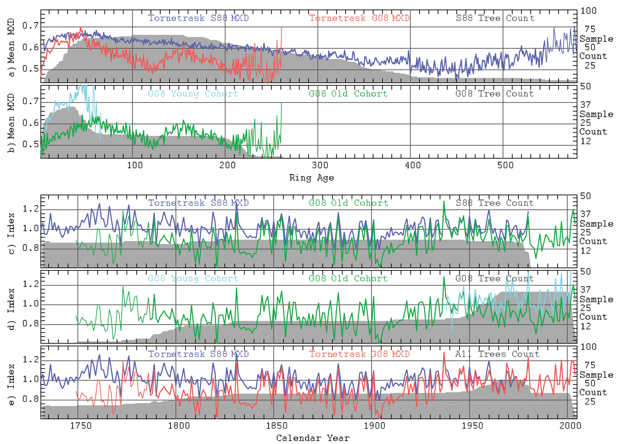
(a) and (b) The mean of maximum latewood density measurements (MXD) for Torneträsk, plotted by ring age for the S88 MXD data in blue, the G08 data in red, the G08 old cohort of trees in green, and the G08 young cohort of trees in cyan. Tree indices were calculated by dividing MXD measurements by the appropriate values of a single RCS curve created using the combined MXD data (S88 and G08). The RCS curve was built from signal-free measurements and smoothed using age-related smoothing. (c), (d) and (e) Chronology indices for the S88 (blue), G08 (red), G08 old cohort (green), and G08 young cohort (cyan) plotted by calendar year. To give some indication of reduced replication the thicker parts of the lines show mean values based on (arbitrarily) four or more samples and the grey shading shows sample counts over time.

MXD adjustment of means and standard deviations

The expected value of a ring measurement is the product of age-related growth rate and chronology value for that year, i.e. RCS value for that ring age multiplied by chronology index. The expected mean value of the data used to update a chronology will be the mean value, for each ring of the update data in the common period, of the expected values calculated using the original chronology. The mean values of the G08 old cohort MXD data were rescaled to match the expected mean value of the original (multiply old cohort MXD values by a calculated factor) over the period 1749 to 1930. The standard deviation of measurement series was adjusted to obtain chronologies with the same standard deviation over their common period (ignoring variation of standard deviation with sample count). The standard deviation was reset by removing the mean, scaling by a factor, and adding back the mean. This resetting was performed iteratively (first adjust mean, then adjust standard deviation) recalculate the chronology and repeat the process until original and update chronologies match over the selected common period. The S88 MXD and adjusted G08 old cohort MXD data were then used to create a combined chronology against which the G08 young cohort MXD data were rescaled as above but using the full period of overlap. The multiplication factor to adjust the G08 old cohort MXD data mean was calculated as 1.19 and, after this mean adjustment, the standard deviation of the old cohort chronology was set to 0.095. The multiplication factor to adjust the young cohort mean was calculated as 1.021 and, after this mean adjustment, the standard deviation of the young cohort chronology was set to 0.074 (see report UpdateG08MXD.prn).

To examine the effect of these adjustments on the MXD data set, the S88 and adjusted G08 data (referred to as G08A data) were used to build an RCS curve and this single RCS curve was used to detrend tree measurements and create series of tree indices using the signal-free method. The mean values of signal-free S88 and G08A measurements are plotted by age in Figure 2a and b. The tree indices for the S88, G08A, G08oA old cohort and G08yA young cohort data sets were averaged into separate mean chronologies and are plotted in Figure 2c, d and e.

OPEN IN VIEWER

Figure 2.

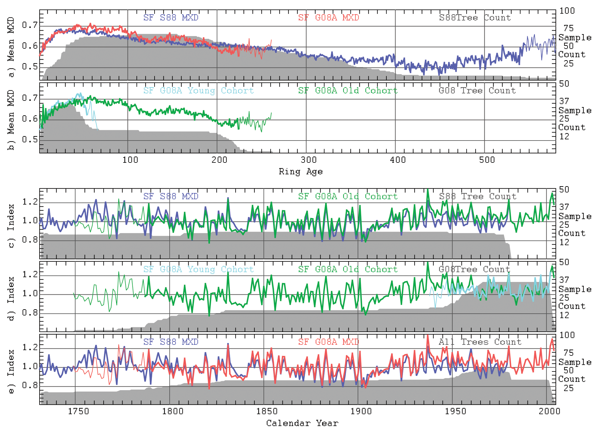
(a) and (b) The mean signal-free maximum latewood density (MXD) by ring age for Torneträsk, for the S88 MXD data in blue, the adjusted G08A data in red, the adjusted G08oA old cohort of trees in green, and the adjusted G08yA young cohort of trees in cyan. Tree indices were calculated by dividing MXD measurements by the appropriate values of a single RCS curve created using the combined MXD data (S88 and adjusted G08A). The RCS curve was built from signal-free measurements and smoothed using age-related smoothing. (c), (d) and (e) Means of tree indices for the S88 (blue), adjusted G08A (red), adjusted G08oA old cohort (green), and adjusted G08yA young cohort (cyan) plotted by calendar year. Adjustments were made to the G08 old cohort data by resetting means and standard deviations to match those of the S88 data (see text for details) over the period 1749 to 1930. The G08 young cohort means and standard deviations were then adjusted to match the combined S88 and G08A old cohort data. The thicker parts of the lines show values based on four or more samples and the grey shading shows sample counts over time..

Mean measurements of the G08A data are similar, when plotted by ring age, to those of the S88 data (Figure 2a). Mean indices of the G08oA old chronology and the G08yA young chronology are similar over their common period (with >4 replication). It can be seen that the uneven decay of the mean MXD of the G08oA old cohort data plotted by age (green) is much reduced as signal-free measures (Figure 2b) in comparison to the measurements containing common signal (Figure 1b). The chronologies from the S88 data (blue) and G08oA old cohort data (green) in Figure 2c are similar up to 1930 and differ after 1930; as expected simple rescaling has not corrected this problem. The G08 old cohort chronology and the G08A young cohort chronology match reasonably well (Figure 2d) as do the S88 chronology and the G08A chronology (Figure 2e). Adjustment of the mean and standard deviation of the G08 old cohort is justified on the basis of the different parameters and machine used in the MXD measuring process. The expectation is that the same adjustment would be needed for the G08 young cohort as they were measured on the same machine. Had the G08 young cohort been a sample from young trees of varying growth rate it would be hoped that the mean measurements would be consistent, i.e. they would need the same adjustment as the G08 old cohort. The G08 young cohort trees were the fastest growing trees of their age class. The assumption that the G08 young cohort experienced similar climate variability to that the G08 old cohort experience justifies the different scaling factor used for the G08 young cohort. The results shown in Figure 2 suggest that the combined S88 and G08A adjusted MXD data set can be considered a homogeneous data set for the purposes of RCS processing.

Analysis of new MXD measurement series

One or two RCS curves MXD

The 124 samples of S88 and adjusted G1112 MXD measurements were standardised using one RCS curve and alternatively using two RCS curves. The resulting mean signal-free MXD by age (unsmoothed RCS curves) are displayed in Figure 3a. For two-RCS-curve standardisation, the two separate chronologies from ‘high’ and ‘low’ value MXD series are compared in Figure 3b and the two-RCS-curve chronology is compared with the one-RCS-curve chronology in Figure 3c. The chronologies were filtered with a 100 year low pass cubic spline for display purposes. The high and low RCS chronologies show similar patterns of low-frequency variance at their recent end where counts for each are above ten samples. In earlier periods counts are lower and the differences between the chronologies are larger while both chronologies show similar patterns of variance. The main reduction in amplitude resulting from using two RCS curves is apparent from ad 800 to 1100 with little change to the chronology after 1500. The young cohort MXD data have already been scaled to match, so there is no sampling bias to correct. One problem is that the limited replication in these data restricts the accuracy of estimation of the low-frequency common signal and the pre-500 data are particularly poorly replicated.

OPEN IN VIEWER

Figure 3.

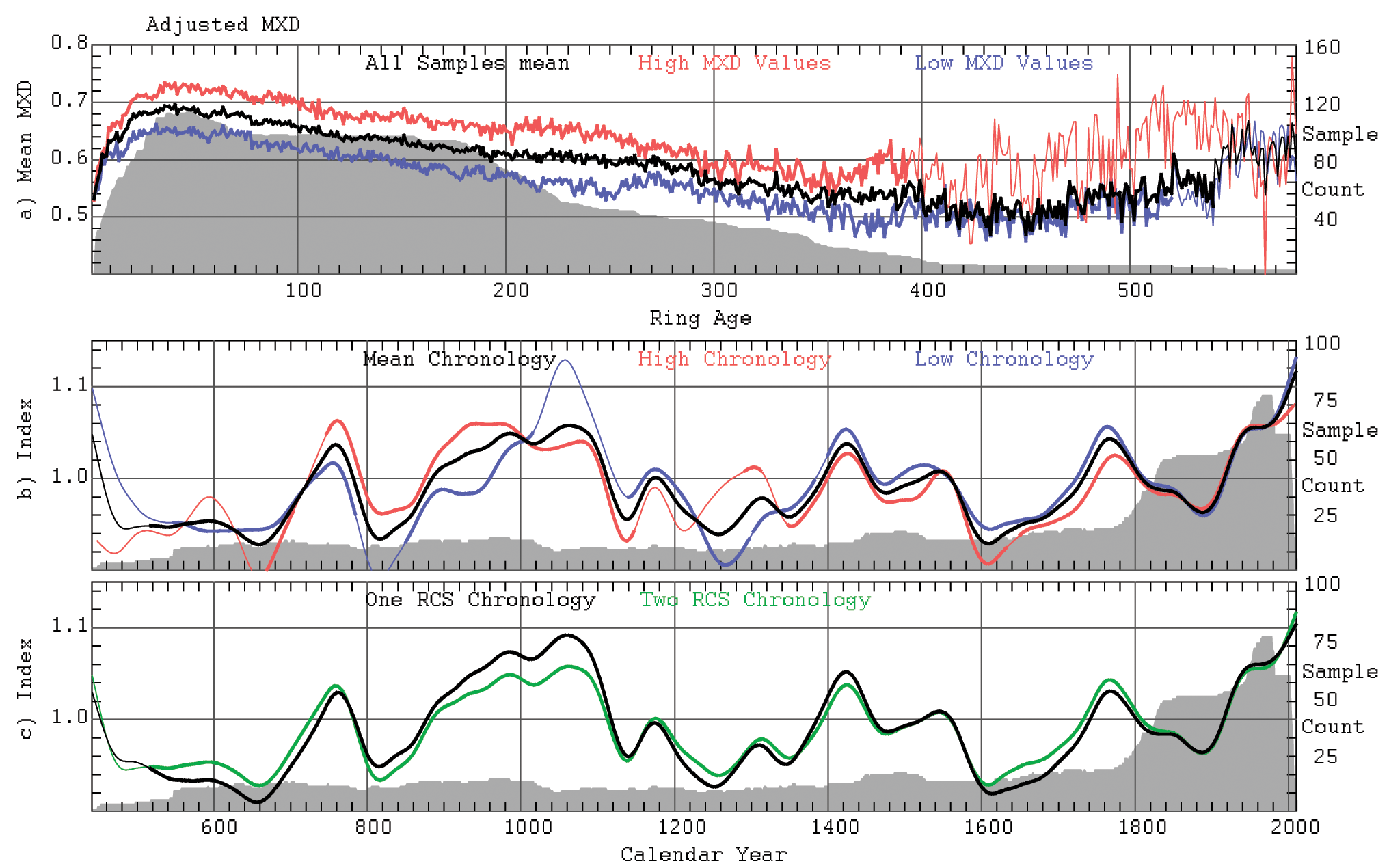
The mean of signal-free MXD measurements plotted by ring age for the combined S88 and G08A MXD data (a). The black curve is based on all samples and the curves in red and blue were built from samples with the highest and lowest values of MXD, respectively, where sorting was based on comparison of mean signal-free MXD against that of a single RCS curve over their common period. (b) Mean chronologies created using two RCS curves; for high-MXD samples (red), low-MXD samples (blue), and the average of all samples (black). (c) Chronologies created using a single RCS curve (black) and two RCS curves (green). Chronologies were low-pass filtered using a 100 year cubic spline. The thicker parts of the lines show sections of chronologies based on four or more samples and grey shading shows the sample counts over time.

Comparison between new and previously published Torneträsk chronologies

Figure 4 illustrates various published TRW and MXD chronologies produced using different subsets of data and different implementations of RCS. Figure 4a shows the TRW (blue), unadjusted MXD (green), and the adjusted MXD (red) chronologies published by Briffa et al. (1992). Figure 4b shows the TRW chronology published by Grudd et al. (2002). Figure 4c shows chronologies created here using S88 MXD data and those TRW data with pith offset estimates (similar to those in Briffa and Melvin, 2011). Figure 4d shows the (S88G08) MXD chronology and the 620-tree TRW chronology (similar to Grudd, 2008), both produced using a single RCS curve. Figure 4e shows the chronologies created here with one RCS curve using the adjusted (S88G08A) MXD data and the 620-tree TRW data. Figure 4f shows the chronologies created here with two RCS curve using the adjusted (S88G1112A) MXD data and the 650-tree TRW data. All chronologies are shown similarly scaled (i.e. by subtraction of the mean and division by the standard deviation) using the yearly data over the period 500–1500 and then smoothed with a 100 year low-pass spline for display purposes.

OPEN IN VIEWER

Figure 4.

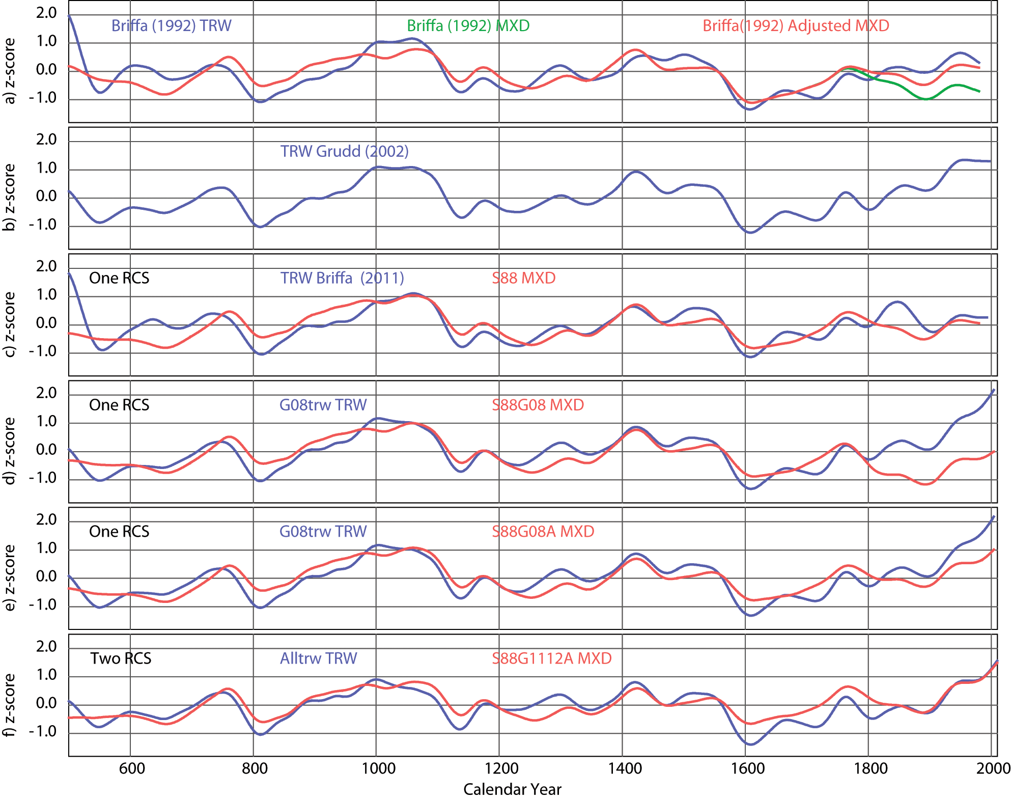
Various Torneträsk chronologies: (a) the TRW, MXD and adjusted MXD chronologies from Briffa et al. (1992); (b) TRW chronology from Grudd et al. (2002); (c) chronologies created using S88 MXD data and TRW data with pith offset estimates (similar to Briffa and Melvin, 2011); (d) chronologies created using the S88G08 MXD data (red), the 620 tree ‘G08trw’ data (blue) from Grudd (2008); (e) chronologies created using the ‘S88G08A’ adjusted MXD data (red) and the 620 TRW trees (blue); and (e) chronologies created using the ‘S88G1112A’ adjusted MXD data (red) and the 650 trees ‘alltrw’ data (blue) . For (a) and (b) chronologies from published papers, for (c) to (e) chronologies were created using one RCS curve, and for (f) chronologies were created using two RCS curves. In all cases chronologies are scaled (by subtracting the mean and dividing by the standard deviation) over the common period ad 500 to 1500 and then low-pass filtered with a 100 year spline for display.

All of these low-frequency chronologies show generally consistent variability up until about 1800. The unadjusted MXD chronology (Figure 4d, red) is distinctly lower after 1800 relative to its earlier long-term average. The adjustment to the MXD data (Figure 4e, red) corrects this problem caused by the difference in mean values of the original (S88) measurements and measurements of the updating samples (either the G08 or G1112) to provide MXD chronology values consistently above the long-term average during the last 100 years. Using a single RCS curve to process the TRW data used by Grudd (2008) produces recent chronology values slightly higher than those produced by Grudd et al. (2002) (though the latter data ended in 1997). However, the adjusted MXD are still considerably below the TRW after 1900 (Figure 4e). Reprocessing all of the updated TRW data, using two RCS curves, reduces the magnitude of the post-1900 TRW chronology (Figure 4f, blue) compared with the single RCS version (as produced in Grudd, 2008) and the updated TRW and MXD low-frequency variability now correspond more closely. This is in part because of a reduction in ‘modern sample bias’ in the new TRW chronology. It should be stressed that the processing and adjustment of the MXD data were done independently of that for the TRW data and the correspondence in recent trends is not because one has been adjusted to fit the other.

Three sets of meteorological measurement series of mean monthly temperatures are available; Abisko station data from the Torneträsk region for the 1913 to 2010 period (provided by Abisko Scientific Research Station http://www.polar.se/abisko); a long composite data set, Bottenviken, covering the period 1860 to 2006 which had been developed for northern Sweden (Alexandersson, 2002); and a long composite data set, Tornedalen, from northern Sweden (Klingbjer and Moberg, 2003). Grudd (2008) found problems with the early Tornedalen data which had not been adjusted pre- and post-introduction of Stevenson screens and may be biased prior to 1850. Here we use the Abisko and Bottenviken temperature series to explore the relationships between recorded temperatures and the two-RCS-curve TRW and MXD chronologies. Published analyses of the detailed character of the tree-growth response to temperature variability in this region show different seasonal optimum associations with temperature for ring-width and density data: TRW being more strongly associated with July and June while MXD data correspond better with a longer April–September season (Briffa et al., 2002). Significant relationships are apparent, for both individual months and for series of means of adjacent months (see Figure S19, available online). The May–August mean temperature series from the longer Bottenviken temperature series show high correlations against both TRW and MXD chronologies and this was selected for ‘climate reconstruction’ using simple regression (see SM18, available online, for details).

Figure 5 shows the temperature reconstructions generated by regressing TRW (a) and MXD (b) chronologies against Bottenviken mean May–August temperature measurements. The two-standard-error confidence range of the chronologies (see SM15, available online, for details) scaled to the reconstructions are also shown (note: low sample replication after 2008, i.e. only five trees are considered insufficient to represent a reliable reconstruction). A full analysis of the reconstruction errors is not attempted here. Over the calibration period, the root-mean-squared error for MXD is 0.60°C and for TRW is 0.9°C. The reconstruction error will be larger than this during periods when the chronology confidence range is wider. The superior replication of the TRW samples results in considerably narrower confidence limits on the TRW chronology but the TRW has less skill at predicting high-frequency temperature variance. The MXD and TRW regressions explain 70% and 32% of the variance, respectively. To highlight the common period with climate the chronology data are plotted in Figure 5d and e along with the mean May–August temperatures from1860 to 2006. The TRW and MXD series have been normalised over the common period 600 to 2008 and then smoothed with a 10 yr spline and are compared in Figure 5c. Within the limits of error produced by low replication, these smoothed chronologies are very similar over their common period and present essentially the same view of past tree-growth variations and inferred summer temperature change at medium and long timescales. The MXD reconstruction will be a superior proxy for examining the high-frequency variance of summer temperature from ce 800 onwards. If 10 yr low-pass (or more smoothed) data are required then either an average of the TRW and MXD reconstructions (post ce 800) or the TRW reconstruction (post ce 200) can be used.

OPEN IN VIEWER

Figure 5.

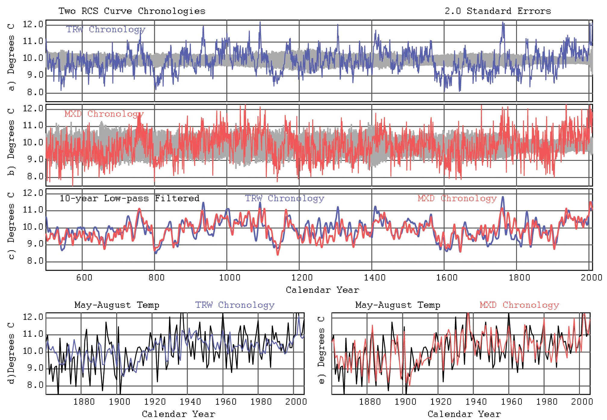
Temperature reconstructions created using the 650-tree (‘alltrw’ data) TRW chronology (a) and the 130 tree (‘S88G1112’ data) MXD chronology (b). Chronologies were created using two RCS curves and were regressed against the Bottenviken mean May–August monthly temperature over the period 1860 to 2006. The shaded areas show two standard errors (see SI15, available online, for details) plotted either side of the mean where standard errors were scaled to fit the temperature reconstruction. The TRW and MXD temperature reconstructions of (a) and (b) are compared in (c) after they were normalised over the common period 600 to 2008 and smoothed with a 10 year spline. The lower two panels compare the reconstructions using the TRW chronology (d) and MXD chronology (e) with the mean of May to August monthly temperature from Bottenviken over the period 1860 to 2006.

If the good fit between these tree-growth and temperature data is reflected at the longer timescales indicated by the smoothed chronologies (Figures 5c and S20d, available online), we can infer the existence of generally warm summers in the 10th and 11th centuries, similar to the level of those in the 20th century. Shorter warm periods appear to have occurred in the mid 8th century, the early 15th century and the mid 18th century. Cool conditions prevailed from the late 16th to the end of the 17th century and shorter cool periods include the early 9th century, the mid 12th century, the early 19th century, and in the early 20th century, with TRW data perhaps implying somewhat greater amplitude of cooling at these times depending on the manner of chronology scaling. These conclusions, and the evidence of comparatively similar warmth in medieval and recent century summers, are in accord with earlier temperature inferences based on RCS processing of these or similar earlier Torneträsk data (Briffa et al., 1992; Grudd et al., 2002). However the new results contradict the evidence presented by Grudd (2008) that northern Fennoscandia ‘may have been considerably warmer than previously recognised’ during medieval times and significantly warmer as compared with the late-twentieth century. That analysis showed (April–August mean) medieval temperatures some 1°C above the late 20th century mean values (Grudd, 2008: figure 11) whereas the results here imply a level of recent summer temperatures that is equivalent, though not yet as persistent over as long a period, to the warmth in medieval time.

Finally we re-iterate that the use of two-RCS-curve processing may reduce the total amplitude of the chronology series and perhaps reduce the magnitude of high relative tree growth in the medieval and modern eras (c.f. Figure 3c). The latter is justified, however, because of the need to reduce the effect of modern sample bias in the chronologies. The poor general level of replication of the MXD, regardless of the form of RCS processing leads to wider confidence levels on the MXD chronology (which is not sufficiently replicated prior to ce 500 or after 2008) while the association between modern instrumental measurements and chronology variability is superior for the MXD compared with the TRW series.

Conclusions