East Asian summer monsoon precipitation variations in China over the last 9500 years: A comparison of pollen-based reconstructions and model simulations

Abstract

To better understand the long-term changes of the East Asian summer monsoon precipitation (P_jja), quantitative reconstructions and model simulations are needed. Here, we develop continental-scale pollen-based transfer functions for P_jja with weighted averaging–partial least squares (WA-PLS) regression and a Bayesian multinomial regression method. We apply these transfer functions to a set of fossil pollen data from monsoonal China for quantitatively reconstructing the P_jja changes over the last 9500 years. We compare the reconstructions with P_jja simulations from a coupled atmosphere–ocean–sea ice general circulation model (the Kiel Climate Model, KCM). The results of cross-validation tests for the transfer functions show that both the WA-PLS model (r² = 0.83, root mean square error of prediction (RMSEP) = 112.11 mm) and the Bayesian model (r² = 0.86, RMSEP = 107.67 mm) exhibit good predictive performance. We stack all P_jja reconstructions from northern China to a summary curve. The stacked record reveals that P_jja increased since 9500 cal. yr BP, attained its highest level during the Holocene summer monsoon maximum (HSMM) at ~7000–4000 cal. yr BP and declined to present. The KCM output and the reconstructions differ in the early-Holocene (~9500–7000 cal. yr BP) where the model suggests higher P_jja than the reconstructions. Moreover, during the HSMM, the amplitude of the P_jja changes (~20–60 mm above present) in simulations is lower than the reconstructed changes (~70–110 mm above present). The rising (declining) P_jja patterns in reconstructions before (after) the HSMM are more pronounced and fluctuating than in simulations. Other palaeohydrological data such as lake-level reconstructions indicate substantial monsoon precipitation changes throughout the Holocene. Our results therefore show that the KCM underestimates the overall amplitude of the Holocene monsoon precipitation changes.

Keywords

climate model climate reconstructions East Asian summer monsoon monsoonal China pollen data precipitation

Introduction

The East Asian summer monsoon circulation is one of the most important components of the Earth’s climatic system and exerts significant effects on the Earth’s energetic and hydrologic cycles (e.g. Dykoski et al., 2005; Wang et al., 2008; Webster et al., 1998). The summer monsoon precipitation plays a crucial role in maintaining the livelihood and well-being of the densely populated monsoonal region of China since it not only provides essential rainfall for supporting agricultural production and sustaining natural ecosystem but also varies strongly in time and can thus cause severe periods of floods and droughts that affect social and economical activities in China (e.g. Peng et al., 2005; Tan et al., 2009; Webster, 2006). Therefore, understanding the long-term variability of the monsoon precipitation in the past, particularly during the Holocene, is vital both for characterizing the contemporary monsoon precipitation patterns and for predicting the future monsoon dynamics.

In southern China, the Holocene variability of the summer monsoon precipitation has been mostly inferred from well-dated speleothem δ¹⁸O records (e.g. Dong et al., 2010; Hu et al., 2008; Jiang et al., 2012; Wang et al., 2001; Yuan et al., 2004). These records have shown that the monsoon precipitation increased since the beginning of the Holocene, reached the maximum extent during the early-Holocene and declined over the last several millennia. This general trend roughly follows the overall orbitally induced variations in summer insolation of the Northern Hemisphere (e.g. Kutzbach, 1981; Ruddiman, 2008; Wang et al., 2010). In contrast, in central and northern China, the Holocene variability of the summer monsoon precipitation displays a different pattern (e.g. An et al., 2000; Lu et al., 2013; Wang et al., 2014; Xie et al., 2013). For example, Cai et al. (2010) showed that the overall rising trend of the speleothem δ¹⁸O value during the Holocene, reflecting the termination of the monsoon precipitation maximum, started earlier in the low-latitude regions, for instance at ~7000 cal. yr BP in the Dongge Cave record, whereas this shift commenced at ~4500 cal. yr BP in the Jiuxian Cave record in central China. Peng et al. (2005) employed a grain-size record of Lake Daihai from northern China to reconstruct the Holocene monsoon precipitation changes and revealed that the precipitation was low before ~7900 cal. yr BP, attained the highest extent during the middle-Holocene from ~7900 to ~3100 cal. yr BP and decreased to present. It is therefore likely that the spatiotemporal patterns of the monsoon precipitation over the Holocene vary between southern and northern China.

Although a large number of qualitative studies on the Holocene monsoon precipitation changes are available, there has been a lack of quantitative Holocene monsoon precipitation data from China. To numerically explore the Holocene variability of the monsoon precipitation, it is essential to obtain high-resolution quantitative reconstructions from different parts of monsoonal China. Fossil pollen spectra preserved in lake or peat sediments have been recently employed as a robust proxy for quantitative climate reconstructions in China (e.g. Jiang et al., 2010; Li et al., 2014a; Sun and Feng, 2013; Xu et al., 2010), mostly focusing on variables such as annual precipitation, annual average temperature and July average temperature. In addition, state-of-the-art coupled climate models can yield quantitative palaeoclimatic data and have been applied to explore the variability of the Holocene monsoon precipitation in China (e.g. Chen et al., 2010; Dallmeyer et al., 2013; Liu et al., 2003). These model studies have mostly focused on different snap-shot experiments, and only a few transient model outputs spanning most of the Holocene are available. Recently, Jin et al. (2014) applied a coupled atmosphere–ocean–sea ice general circulation model (the Kiel Climate Model (KCM)) to conduct a transient simulation for the monsoon precipitation over the last 9500 years, showing that the monsoon precipitation patterns differ regionally in China.

The comparison of proxy-based quantitative climate reconstructions and model-based climate simulations has been demonstrated to be an effective approach for evaluating the accuracy and reliability of the model simulations and for identifying the main forcing and feedback mechanism of past climate changes (e.g. Braconnot et al., 2012; Brewer et al., 2007; Masson et al., 1999; Mauri et al., 2014; Prentice et al., 1998; Renssen et al., 2009). Here, we present new quantitative reconstructions for the Holocene summer monsoon precipitation from monsoonal China. We first establish robust pollen-based transfer functions for the monsoon precipitation with the continental-scale Chinese surface pollen dataset (Zheng et al., 2008) and apply these transfer functions to a set of Holocene pollen sequences obtained from lake or peat sediments. We then compare in detail our monsoon precipitation reconstructions with the recently published monsoon precipitation simulations from the KCM (Jin et al., 2014). We aim to provide quantitative information on the Holocene monsoon precipitation changes and gain more insights into its spatial and temporal variability with data–model comparison.

Materials and methods

Modern and fossil datasets

For modern datasets, we employed a continental-scale set of surface pollen data over China which has been described in detail by Zheng et al. (2008, 2014) and Li et al. (2014a, 2015). It contains 1374 samples covering all major climatic and vegetation zones of continental China (Figure 1a). We calculated percentage values for pollen taxa from the total number of terrestrial pollen grains. We derived modern values of the East Asian summer (June, July and August) monsoon precipitation (P_jja) for all surface and fossil pollen sets (see below) from the WorldClim database with a 30-arc-second spatial resolution (Figure 1b; Hijmans et al., 2005).

Figure 1.

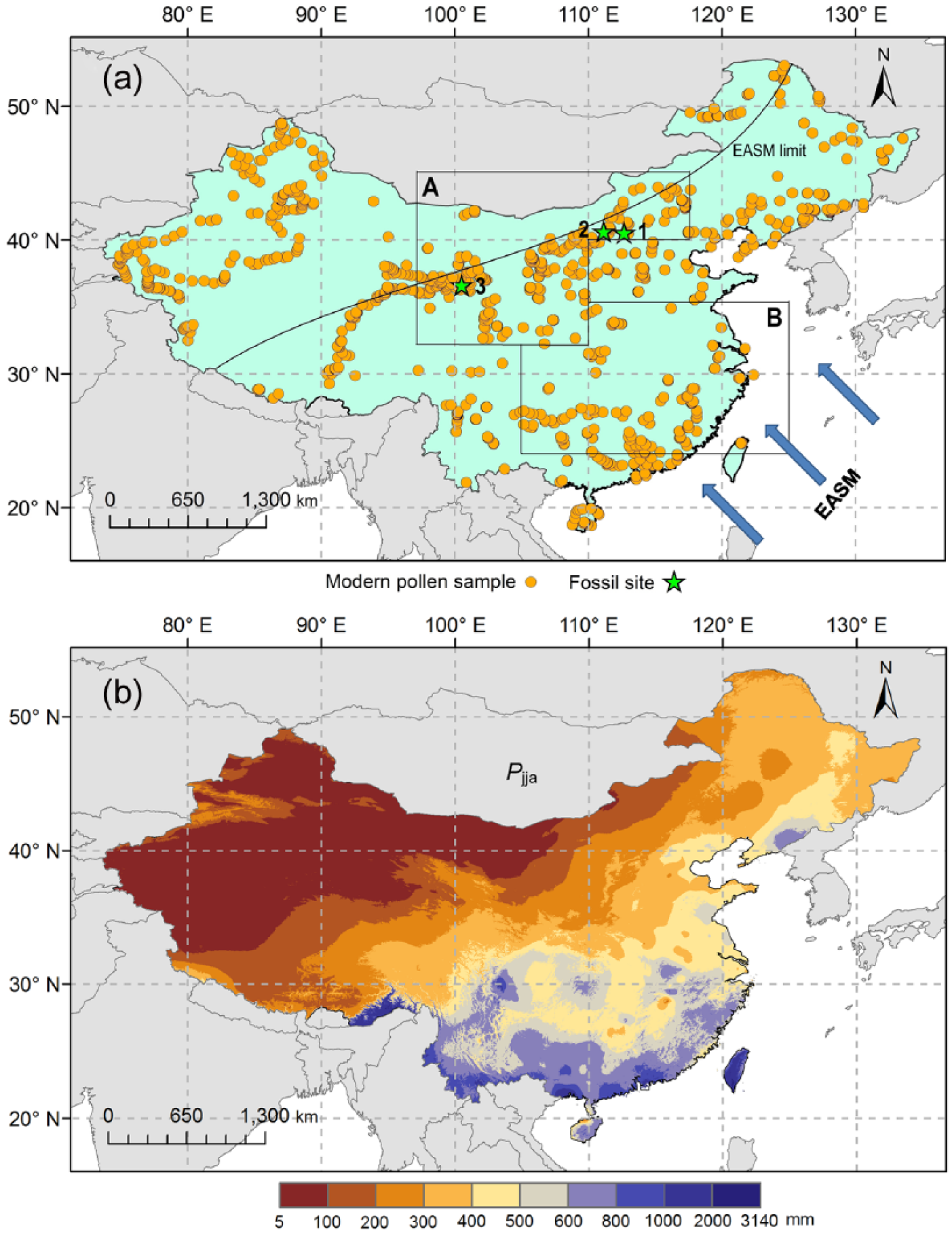
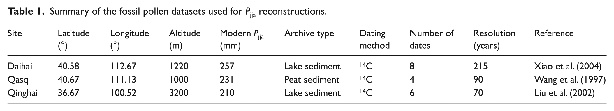
(a) Locations of modern pollen samples and fossil pollen sites: 1 – Daihai, 2 – Qasq and 3 – Qinghai. (b) Modern summer (June, July and August) precipitation (P_jja) of China (Hijmans et al., 2005). Regions A and B are divided after An et al. (2000) and correspond to Regions B and E defined in Jin et al. (2014).

For fossil datasets, we used three previously published pollen sequences from two lakes (Daihai and Qinghai) and one peatland (Qasq), located in the monsoonal region of China (Table 1; Figure 1a). We obtained pollen data for Qinghai and Qasq from the eastern Asian late-Quaternary pollen dataset compiled by Cao et al. (2013) and for Daihai from Xiao et al. (2004) and Xu et al. (2010). We selected these fossil pollen datasets because they have more reliable chronology and higher temporal resolution than most of the other published pollen data from monsoonal China (Table 1). The chronology of the fossil sequences is obtained on the basis of AMS radiocarbon dating. The number of AMS ¹⁴C dates per sequence varies between 4 and 8 (Table 1). We calibrated all ages to calendar years according to the IntCal09 calibration dataset (Reimer et al., 2009) and reestablished age–depth models for all sites (Appendix 1, available online) using the CLAM package (Blaauw, 2010) in R (R Development Core Team, 2012).

Table 1.

Summary of the fossil pollen datasets used for P_jja reconstructions.

Site	Latitude (°)	Longitude (°)	Altitude (m)	Modern P_jja (mm)	Archive type	Dating method	Number of dates	Resolution (years)	Reference
Daihai	40.58	112.67	1220	257	Lake sediment	¹⁴C	8	215	Xiao et al. (2004)
Qasq	40.67	111.13	1000	231	Peat sediment	¹⁴C	4	90	Wang et al. (1997)
Qinghai	36.67	100.52	3200	210	Lake sediment	¹⁴C	6	70	Liu et al. (2002)

KCM output

We extracted the P_jja simulations spanning the last 9500 years from the KCM output for northern China (Region A, corresponding to Region B in Jin et al., 2014) and southern China (Region B, corresponding to Region E in Jin et al., 2014). We defined Regions A (32.5–45°N, 97.5–117.5°E) and B (25–35°N, 105–125°E) (Figure 1a) which include our fossil sites according to Chinese physiography (An et al., 2000) and horizontal resolution used in the KCM simulations (Jin et al., 2014). The KCM (Park et al., 2009) is composed of the European Centre for Medium-Range Weather Forecasts (ECMWF) Hamburg atmospheric general circulation model version 5 (ECHAM5; Roeckner et al., 2003) and the Nucleus for European Modelling of the Ocean (NEMO; Madec, 2008) ocean–sea ice general circulation model, with the Ocean Atmosphere Sea Ice Soil version 3 (OASIS3; Valcke, 2006). The KCM transient simulations were forced primarily by the orbitally induced insolation variations (Berger and Loutre, 1991) and neglected variations of other forcing factors such as greenhouse gas concentrations, ice sheet extents and terrestrial vegetation feedbacks. The difference between the fixed-day and the fixed-angular calendars (Chen et al., 2011) was not corrected for the KCM output, as this has no influence on the simulations because of relatively low eccentricity during the Holocene (Jin et al., 2012). The spatial resolution of the model is T31 (3.75° × 3.75°) with 19 vertical levels. More details of experiment setup and results of the KCM simulations have been described by Jin et al. (2014).

Numerical analyses

We developed quantitative pollen-based transfer functions for P_jja using two different techniques, weighted averaging–partial least squares (WA-PLS) regression (Ter Braak and Juggins, 1993) with five components and a Bayesian regression model.

For the WA-PLS transfer functions, we utilized leave-one-out cross-validation (Birks et al., 1990) to evaluate their model performances and estimated performance statistics such as coefficient of determination (r²) between measured and predicted values, root mean square error of prediction (RMSEP) and maximum bias for each WA-PLS transfer function. We transformed the surface pollen data to square-roots for reducing the noise of the data (Prentice, 1980), applied randomization t-test (Van der Voet, 1994) for selecting the most appropriate WA-PLS component for P_jja reconstructions and calculated sample-specific standard errors for the reconstructions with a bootstrapping procedure with 1000 cycles (Birks, 2003). We performed the WA-PLS transfer functions and associated P_jja reconstructions with the RIOJA package (Juggins, 2012) in R. We assessed statistical significance of the WA-PLS-based P_jja reconstructions with the approach involving 999 randomizations developed by Telford and Birks (2011) and conducted these significance tests with the R package PALAEOSIG (Telford, 2011).

For the Bayesian transfer function, we used Bummer, the Bayesian hierarchical multinomial regression model originally developed for past temperature reconstructions by Vasko et al. (2000). We modified it for the P_jja reconstructions by resetting some prior model specifications. The Bummer model together with its modifications and extensions has been applied to palaeotemperature reconstructions in Korhola et al. (2002), Erästö and Holmström (2006), Salonen et al. (2012) and Holmström et al. (in press). The full methodological description of the Bayesian approach is provided in Appendix 2, available online. The computation time makes leave-one-out cross-validation impracticable for the Bayesian model. Instead, we employed a simplified procedure where a 10-fold cross-validation test was used to evaluate the Bayesian model performance (see Appendix 2, available online, for details). We calculated the performance statistics including r², RMSEP and maximum bias for the Bayesian model. We did not test the statistical significance of the Bayesian-based P_jja reconstructions because of the restrictive calculating demands for computing separate reconstructions with 999 randomizations of climate data. The Bayesian transfer function and associated P_jja reconstructions with error estimates were conducted using the MATLAB software.

Results

Transfer function performance

Performance statistics of the WA-PLS and Bayesian transfer functions for P_jja are presented in Figure 2 and Table 2. The three-component WA-PLS model with an r² of 0.83, RMSEP of 112.11 mm and maximum bias of 174.34 mm was chosen for the P_jja reconstructions because this WA-PLS model has the lowest RMSEP and highest r² among all WA-PLS models, and the addition of higher number of the WA-PLS components did not yield statistically significant improvement (p < 0.05) in the overall model performance, as demonstrated by the results of the randomization t-test (Table 2). The Bayesian transfer function has a higher r² (0.86) and lower RMSEP (107.67 mm) but higher maximum bias (192.96 mm) than the selected WA-PLS transfer function. The scatter plots of predicted P_jja against modern observed P_jja and residuals of predicted P_jja against modern observed P_jja for the selected WA-PLS and Bayesian models are shown in Figure 2. As can be seen, the residuals of both models indicate a slight tendency of an underestimation of P_jja at the high precipitation end of the P_jja gradient.

Figure 2.

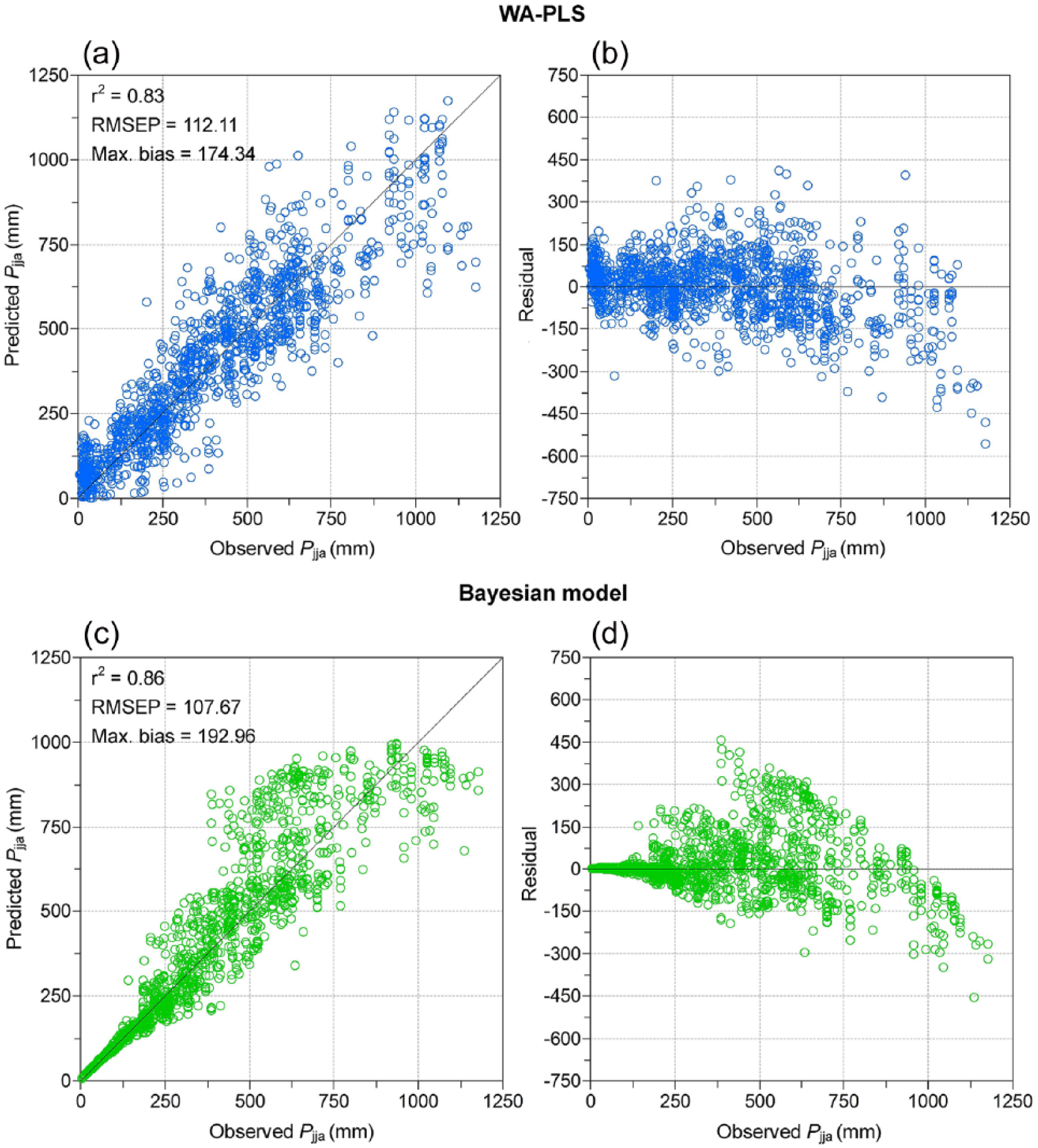
Scatter plots of (a) WA-PLS predicted versus observed P_jja values, (b) residuals of WA-PLS predicted versus observed P_jja values, (c) Bayesian predicted versus observed P_jja values and (d) residuals of Bayesian predicted versus observed P_jja values.

Table 2.

Performance statistics of the pollen–P_jja models with five WA-PLS components.

WA-PLS components	r ²	RMSEP	Maximum bias	t-value
1	0.79	123.56	276.47	–
2	0.82	115.15	261.17	0.001
3	0.83	112.11	174.34	0.009
4	0.83	113.88	169.19	0.976
5	0.82	117.95	195.34	1.000

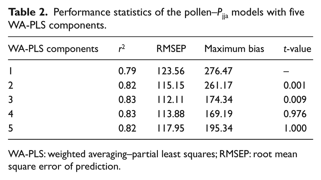
WA-PLS: weighted averaging–partial least squares; RMSEP: root mean square error of prediction.

Quantitative P_jja reconstructions

The quantitative P_jja reconstructions are illustrated in Figure 3. The P_jja reconstructions using the WA-PLS model for the three sites (Daihai, Qasq and Qinghai) from northern China are statistically significant (p < 0.005), as assessed by the Telford and Birks (2011) significance test. The general trends of the Bayesian-based P_jja reconstructions mostly resemble the WA-PLS-based reconstructions. The main differences between reconstructions are that the estimated standard errors in the Bayesian reconstructions are markedly smaller than those in the WA-PLS reconstructions and the absolute reconstructed P_jja values are different especially for Daihai (Figure 3). Site-specific P_jja reconstructions vary individually over the last 9500 years. At Daihai, the Bayesian reconstruction exhibits a lower magnitude of change than the WA-PLS reconstruction because of higher reconstructed P_jja in the early- or late-Holocene and lower reconstructed P_jja in the middle-Holocene. In the WA-PLS reconstruction, P_jja fluctuates around ~280 mm from ~9500 to ~7800 cal. yr BP, reaches the maximum value around 380 mm at ~7400–3600 cal. yr BP and decreases to the lowest value of about 140 mm in the last 1400 years. For Qasq and Qinghai, the overall differences between the Bayesian and WA-PLS reconstructions are small. At Qasq, P_jja displays the minimum value less than 220 mm from ~9500 to ~8200 cal. yr BP, rises to ~380 mm at ~7600 cal. yr BP, attains the highest value around 580 mm between ~4800 and ~2800 cal. yr BP and falls down to the present-day measured value of 231 mm. At Qinghai, P_jja fluctuates around 260 mm at ~9500–8600 cal. yr BP, shows the maximum value of ~300 mm at ~8000–6400 cal. yr BP and declines to the lowest value below 200 mm in the last 1200 years.

Figure 3.

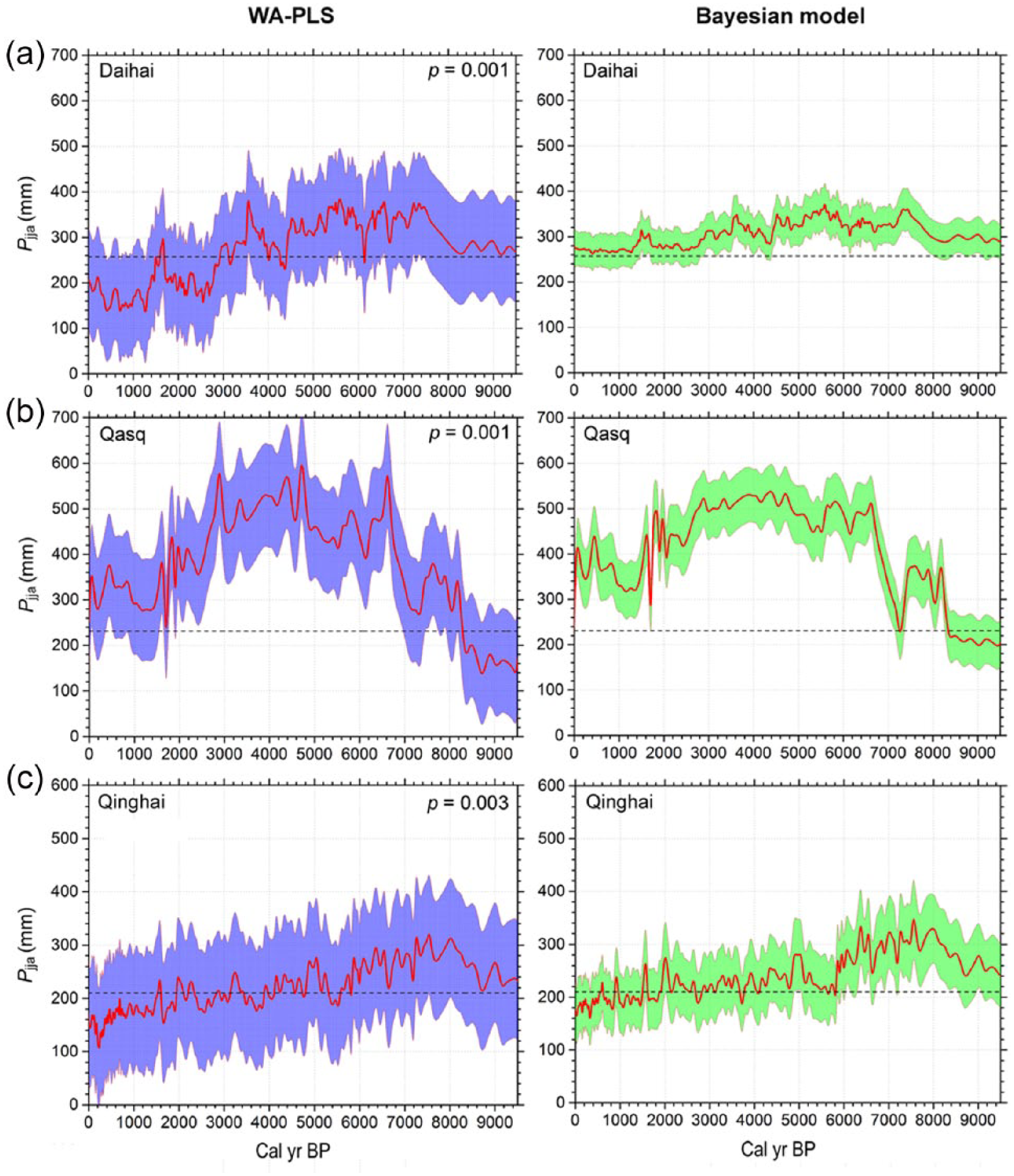
Pollen-based P_jja reconstructions covering the past 9500 years for (a) Daihai, (b) Qasq and (c) Qinghai based on the WA-PLS and Bayesian models. Error bars represent the bootstrap-estimated errors for the WA-PLS reconstructions and the 95% posterior credible intervals for the Bayesian reconstructions. The p-values are shown for each WA-PLS reconstruction assessed in the Telford and Birks (2011) significance test. Modern observed P_jja values for the fossil sites are indicated with horizontal dashed lines.

Comparison to KCM-based P_jja simulations

To highlight the regional patterns of the P_jja reconstructions for northern China (Region A) in comparison with the KCM-based simulations, deviations from the average of the six P_jja reconstructions over the past 9500 years were calculated and stacked together to prepare one curve (Figure 4). The stacked record for Region A shows that P_jja increases since 9500 cal. yr BP, reaches the highest level at ~7000–4000 cal. yr BP and decreases to present. In contrast, the P_jja simulations are more muted (Figures 4 and 5). In northern China (Region A), the simulated P_jja fluctuates around ~350 mm at ~9500–8500 cal. yr BP, increases to the maximum value around ~380 mm at ~8500–6000 cal. yr BP and declines to the lowest value below 250 mm in the last 1200 years (Figure 5). In southern China (Region B), the simulated P_jja shows the maximum value around ~650 mm at ~9500–6500 cal. yr BP, falls down to ~600 mm from ~6500 to ~3500 cal. yr BP, and reaches the lowest Holocene value less than 450 mm during the last 2400 years.

Figure 4.

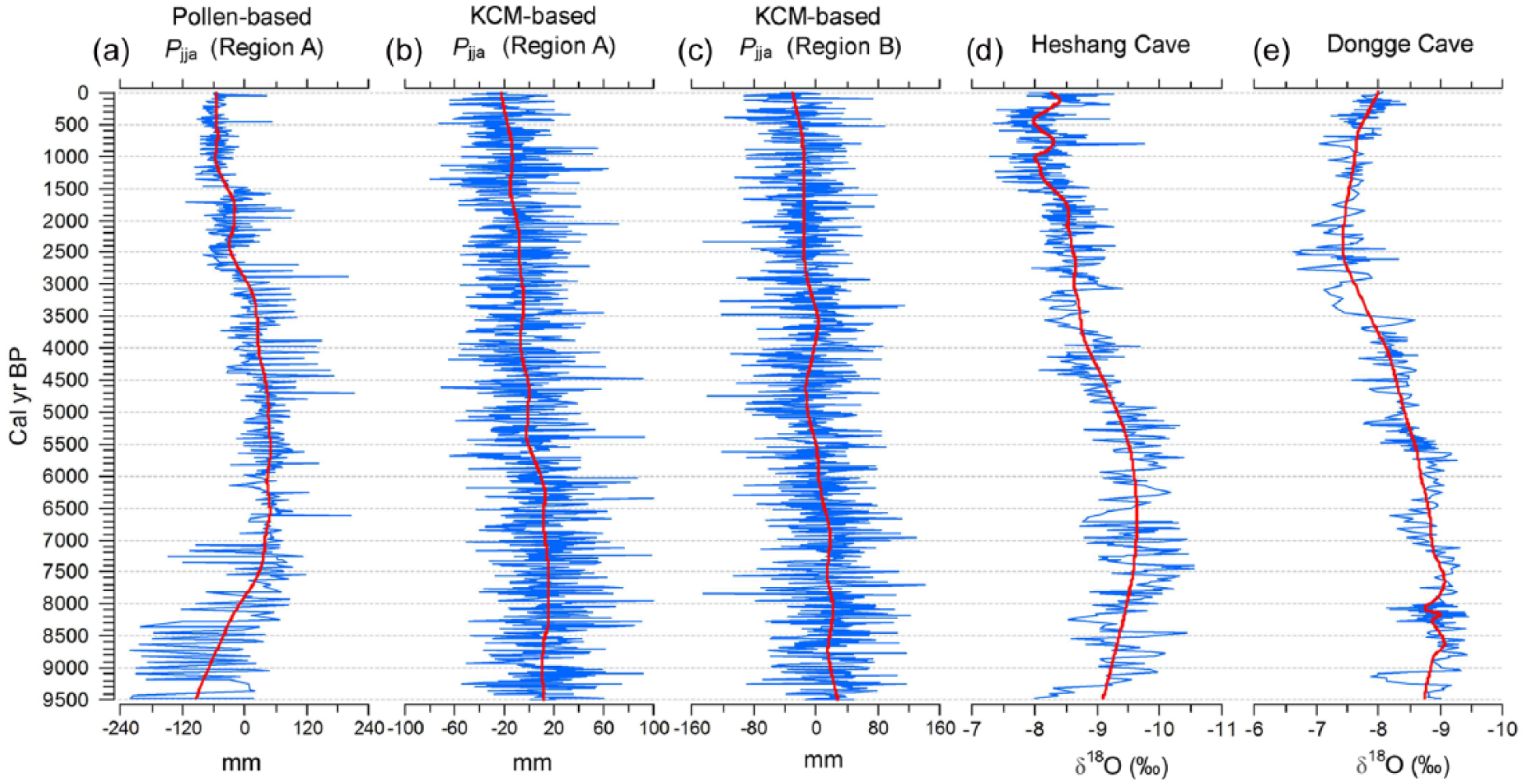
Comparison of (a) pollen-based stacked P_jja record for northern China (Region A) with KCM-simulated P_jja deviations from the Holocene mean (Jin et al., 2014) for (b) northern China (Region A) and (c) southern China (Region B), and speleothem δ¹⁸O records from (d) Heshang (Hu et al., 2008) and (e) Dongge Cave (Dykoski et al., 2005) in southern China. LOESS smoothers with a span of 0.15 are added to all curves.

Figure 5.

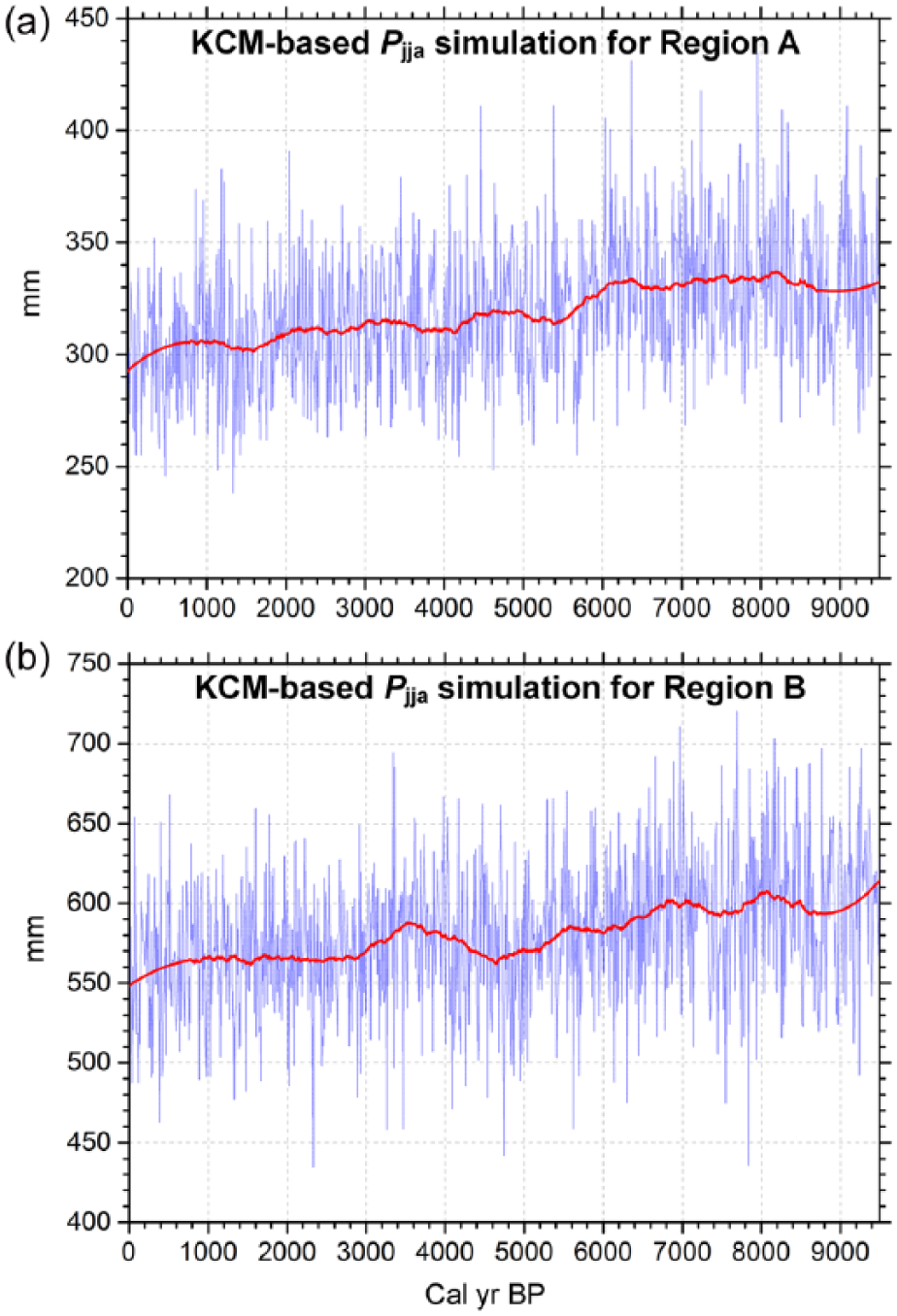
KCM-based P_jja simulations (Jin et al., 2014) for (a) northern China (Region A) and (b) southern China (Region B). LOESS smoothers with a span of 0.1 are added to all curves.

Discussion

Assessment of transfer functions

To assess the reliability of our continental-scale WA-PLS transfer function for P_jja, we compare the performance statistics of our model with one existing regional-scale pollen-based transfer function for P_jja (Wen et al., 2013) and earlier regional- or continental-scale pollen-based transfer functions for annual precipitation (P_ann) from monsoonal Eastern Asia (e.g. Cao et al., 2014; Li et al., 2007, 2014a; Lu et al., 2011). Among all models listed in Appendix 3, available online, the inferred r² value (0.83) of our WA-PLS model for P_jja falls into the upper range of r² values for P_jja or P_ann (0.83–0.89). However, the RMSEP value (112 mm) of our model as a proportion of the gradient length (9.5%) falls into the middle range of RMSEP values for P_jja or P_ann (8.5–9.5%), likely because of long climatic gradient in our study. The slight underestimates for P_jja at wetter sites in the residuals of our WA-PLS model may be caused by edge effects that are inherent to the WA-PLS technique (Birks, 1998).

The Bayesian model somewhat outperforms over the WA-PLS model in terms of performance statistics (Figure 2). This is in line with previous findings from northern Europe where the Bayesian model has been tested and applied for palaeoclimatic reconstructions (e.g. Korhola et al., 2002; Salonen et al., 2012; Toivonen et al., 2001; Vasko et al., 2000). Possible reason is that the Bayesian approach provides many significant advantages compared with the commonly used classical approaches such as WA-PLS (e.g. Korhola et al., 2002; Salonen et al., 2012; Vasko et al., 2000). For example, the Bayesian calibration process is transparent because of the utilization of probability distributions rather than point estimates used by WA-PLS and can therefore provide more information with regard to the taxon responses, model behaviour and uncertainty related to the process. Moreover, ecological knowledge can be explicitly embedded into the Bayesian model and quantified in terms of posterior probability. In addition, the Bayesian approach is capable of taking into account the uncertainty concerning site-specific latent variables (the probabilities in the model) that are not attainable in the classical approaches such as WA-PLS. The error estimations (Figure 3) between the Bayesian and WA-PLS reconstructions are different but not directly comparable because the WA-PLS bootstrapping results only show the robustness of point estimations, while the Bayesian model estimates probability distributions in the first place with a large number of inherent uncertainties (Korhola et al., 2002).

Assessment of pollen-based reconstructions

The reliability of the pollen-based quantitative P_jja reconstructions can be evaluated by comparing them with other palaeohydrological records from the same lakes or peatlands. At Lake Daihai, a lake-level reconstruction shows low level prior to ~8000 cal. yr BP, high level at ~8000–3000 cal. yr BP and low level since ~3000 cal. yr BP (Sun et al., 2009). This coincides with our reconstruction for Lake Daihai (Figure 3). At Lake Qinghai, a high-resolution δ¹⁸O record based on ostracod shells suggests high monsoon precipitation at ~10,000–6000 cal. yr BP and declining or low precipitation after ~6000 cal. yr BP (Liu et al., 2007). This supports our reconstruction for Lake Qinghai, showing high P_jja at ~9500–5800 cal. yr BP and a gradual decline after ~5800 cal. yr BP. At Qasq peat sequence, a pollen-based reconstruction for P_ann using pollen response surface method presents high P_ann at ~5500–2000 cal. yr BP (Wang et al., 1998). This is roughly similar to our reconstruction for Qasq, exhibiting high P_jja at ~4800–2800 cal. yr BP. In summary, our pollen-based monsoon precipitation reconstructions are generally in agreement with other past hydrological records from the same lake or peat sediments.

The accuracy of the pollen-based stacked P_jja record can be assessed by comparing it with earlier synthesized records for Holocene moisture variability in northern China. Our record shows that the monsoon precipitation maximum took place at ~7000–4000 cal. yr BP (Figure 4a), being broadly consistent with other records. For example, Feng et al. (2006) reviewed several types of proxy data from 23 fossil records in northern China, and indicated the middle-Holocene from ~7500 to ~3500 cal. yr BP as the wettest period. Yang et al. (2011) assessed a variety of Holocene proxy records from 15 sites and proposed that northern and northwestern China witnessed a wetter period between ~8000 and ~4000 cal. yr BP. Zhao and Yu (2012) synthesized pollen data from 20 fossil sites from the present monsoon margin region and showed that the Holocene moisture maximum appeared at ~8000–4000 cal. yr BP. In contrast, this pattern is different in southern China where previous reviews based upon multi-proxy palaeoclimatic records suggest that the maximum moisture occurred in the early-Holocene between ~10,000 and ~6000 cal. yr BP (e.g. Herzschuh, 2006; Ran and Feng, 2013; Zhang et al., 2011; Zhao et al., 2009b). Additionally, comparison of our stacked record for northern China with the speleothem δ¹⁸O records from the Heshang Cave (Hu et al., 2008) and the Dongge Cave (Dykoski et al., 2005) in southern China also indicates that the monsoon precipitation maximum occurred earlier in southern China, at ~9500–7000 cal. yr BP in the Dongge Cave and ~8000–5200 cal. yr BP in the Heshang Cave (Figure 4).

Comparison of pollen-based reconstructions and model-based simulations

The absolute P_jja values are roughly comparable between our pollen-based reconstructions and the KCM-based simulations (Figures 3 and 5). In northern China (Region A), the reconstructed P_jja values are in the range of ~100–580 mm and the simulated values in the range of ~250–430 mm. However, the amplitude of the P_jja changes indicated by departures with 200-year intervals is different between the reconstructions and simulations (Figure 6). The pollen-based stacked P_jja departures for northern China fluctuate from ~−35 to ~110 mm, whereas the simulated departures are smaller for northern China (~−5–40 mm) and southern China (~−10–60 mm). In addition, the most noticeable differences between the reconstructed and simulated P_jja departures occur during the Holocene summer monsoon maximum (HSMM). As shown in Figure 6, P_jja in northern China was about ~70–110 mm above present for the reconstructed HSMM, while it was only about ~20–40 mm (northern China) or ~30–60 mm (southern China) higher than at present for the simulated HSMM (~8500–6000 cal. yr BP in northern China or ~9500–6500 cal. yr BP in southern China). Palaeohydrological reconstructions from monsoonal China suggest that lake-level changes between the HSMM and the present have been extremely large, for example, ~60 m at Lake Daihai (Sun et al., 2009), ~100 m at Lake Qinghai (Wang, 1992) and ~25 m at Lake Yema (Shi et al., 2002). It is therefore likely that the P_jja simulations underestimate the real amplitude of the Holocene precipitation change and that the reconstructions are in this sense more realistic.

Figure 6.

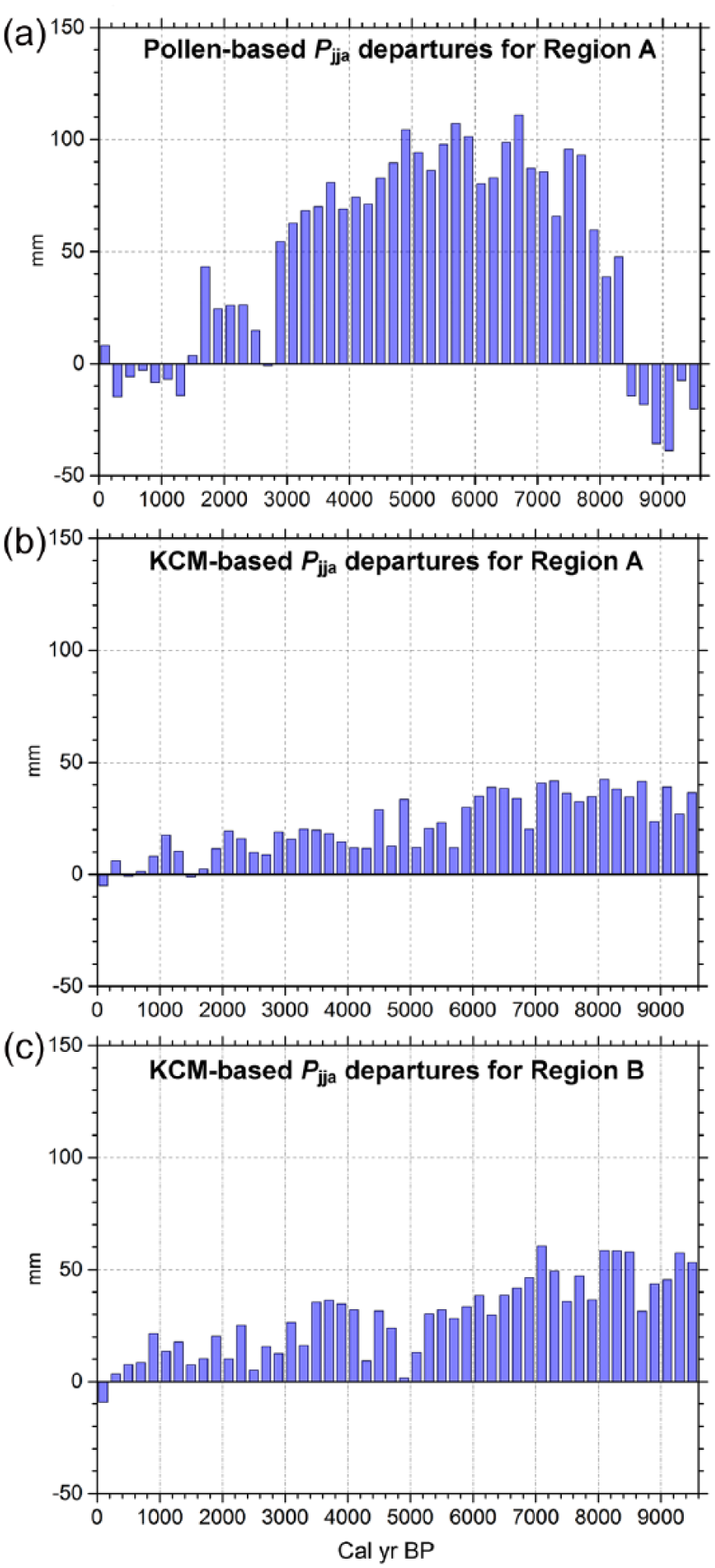
Comparison of (a) pollen-based P_jja departures with 200-year intervals from reconstructed modern P_jja values for northern China (Region A) with KCM-based P_jja departures (Jin et al., 2014) with the same intervals from simulated modern P_jja values for (b) northern China (Region A) and (c) southern China (Region B).

As for the Holocene P_jja trend, the most conspicuous differences between the reconstructions and simulations appear in the early-Holocene between 9500 cal. yr BP and the HSMM (Figures 4 and 5). In northern China, the stacked record shows a rapidly rising trend, while the model simulation displays a moderately increasing trend. The strongly rising monsoon precipitation trend during the period of ~9500–7000 cal. yr BP can be found from many other palaeoclimatic records in northern China (e.g. Chen et al., 2015; Liu et al., 2015; Peng et al., 2005; Wen et al., 2013; Xu et al., 2010; Yang et al., 2011; Zhao et al., 2009a). It is thus likely that the simulated values for the early-Holocene may be too high. The declining P_jja patterns after the HSMM until the present also differ between the reconstructions and simulations (Figures 4 and 5). The simulations exhibit a rather steadily declining trend, while the stacked record shows that P_jja decreased markedly with the most noticeable drop at ~3000 cal. yr BP. The pronounced decreasing monsoon precipitation trend in the middle- and late-Holocene can be detected from other synthesized moisture records (e.g. Ran and Feng, 2013; Yang et al., 2011; Zhao et al., 2009a, 2009b), lake-level reconstructions (e.g. Sun et al., 2009; Wang, 1992) and speleothem δ¹⁸O records (e.g. Cai et al., 2010; Dykoski et al., 2005; Jiang et al., 2012).

Taken together, it is clear that the KCM underestimates the overall Holocene P_jja changes in both magnitude and trend compared with the reconstructions. The main reason can be that the KCM simulations were too strongly driven by the orbitally induced insolation forcing and did not take into account other important forcing factors such as ice sheet volumes and terrestrial vegetation feedbacks (Jin et al., 2014). It is possible that westerly wind was stronger and shifted southward in the early-Holocene compared with the middle-Holocene. This is suggested by low lake levels and moisture contents during the early-Holocene in arid central Asia (e.g. Chen et al., 2008; Ran and Feng, 2013). Such strong westerly airflow would have suppressed the northward penetration of the EASM during the early-Holocene (e.g. Chen et al., 2015; Li et al., 2014; Zhao and Yu, 2012). Chen et al. (2015) suggested that the enhanced westerly circulation would have been linked to the remnant Laurentide ice sheet in northern America that persisted until ~7000 cal. yr BP and provided continuous freshwater input to the North Atlantic (e.g. Barber et al., 1999; Carlson et al., 2008; Renssen et al., 2009). The model simulations by Chen et al. (2015) showed that during the early-Holocene, the intensified North Atlantic freshening would have caused a weaker Atlantic Meridional Overturning Circulation, which in turn would have resulted in the strengthening of meridional temperature gradient and westerly circulation, eventually leading to the depressed insolation-driven EASM in northern China. The connection between a weak Asian summer monsoon and cold events in the North Atlantic during the early-Holocene has also been suggested by many other studies (e.g. Li et al., 2014; Liu et al., 2013; Wang et al., 2005). However, the effect of deglaciation was not taken into account in the KCM simulations. From the HSMM to the present, the decreasing P_jja trends in our pollen-based reconstructions are more pronounced than the simulations. This may be due to that Holocene vegetation in northern China is sensitive to monsoon precipitation change (e.g. Chen et al., 2006; Song et al., 1997; Wu et al., 1994) and that positive feedbacks between vegetation and climate tend to amplify the effect of orbital forcing (e.g. Claussen, 2009; Claussen et al., 1999; Foley et al., 1994; Ganopolski et al., 1998). However, the role of vegetation–climate feedbacks was not considered in the KCM simulations. In addition, the simulated HSMM for southern China took place earlier than the simulated or reconstructed HSMM for northern China, as also highlighted by the comparison of our P_jja data with the speleothem δ¹⁸O data from southern China (Figure 4). As with the weak EASM in northern China during the early-Holocene, this can be attributed to the blocking effect of the strong westerly wind (e.g. Chen et al., 2015; Ding et al., 1994, 2005; Li et al., 2014; Ruddiman, 2008; Wang, 1999; Zhao and Yu, 2012). It is also possible that the Holocene speleothem δ¹⁸O records from southern China mainly reflect the variations of moisture source from the Indian summer monsoon region rather than the East Asian summer monsoon (e.g. Chen et al., 2014; Liu et al., 2015; Wang et al., 2014; Yang et al., 2014).

Conclusion

In this study, we present new pollen-based transfer functions for the East Asian summer monsoon precipitation (P_jja) established with WA-PLS and Bayesian regression methods. The WA-PLS and Bayesian transfer functions have good statistical performances and robust predictive power. We apply these two different models to three fossil pollen records from monsoonal China to reconstruct the quantitative P_jja variations for the last 9500 years. The WA-PLS-based reconstructions from northern China are statistically significant and are generally consistent with the Bayesian-based reconstructions. We combine the individual reconstructions from northern China to one summary record, showing that P_jja increased dramatically between ~9500 and ~7000 cal. yr BP, reached the highest Holocene level from ~7000 to ~4000 cal. yr BP and declined progressively over the past 4000 years. This general pattern agrees with earlier synthesized Holocene moisture records from northern China. We compare our reconstructions with the P_jja simulations from the KCM output. The absolute P_jja values in the reconstructions and simulations are roughly comparable. The major discrepancies are related to the amplitude of the P_jja changes and the overall trends. During the HSMM, P_jja was ~70–110 mm higher than at present in the stacked record, while it was only ~20–60 mm above present in the model results. Furthermore, the increasing or declining P_jja patterns before or after the HSMM in the stacked record are more pronounced than in the simulations. Other palaeoclimatic data reveal significant monsoon precipitation changes during the Holocene. Our data–model comparison therefore suggests that the KCM simulations underestimate the magnitude of the Holocene P_jja changes and the reconstructions are more realistic.

Footnotes

Acknowledgements

We sincerely thank two anonymous reviewers for their constructive comments.

Funding

This work was financially supported by the Strategic Priority Research Program of the Chinese Academy of Sciences (XDA05120202), the Key National Natural Science Foundation of China (grant no. 40730103), the National Natural Science Foundation of China (grant nos. 40730103, 41371215) and the Key Technology R&D Program of Hebei Province (13277611D). JL also greatly acknowledges the financial support by the China Scholarship Council (CSC) for PhD study (grant no. 201208130087) at the University of Helsinki. HS acknowledges the financial support from the project EBOR from the Academy of Finland and the Nordic top-level research initiative CRAICC.

References

Porter

Kutzbach

. (2000) Asynchronous Holocene optimum of the East Asian monsoon. Quaternary Science Reviews 19: 743–762.

Barber

Dyke

Hillaire-Marcel

. (1999) Forcing of the cold event of 8,200 years ago by catastrophic drainage of Laurentide lakes. Nature 400: 344–348.

Berger

Loutre

(1991) Insolation values for the climate of the last 10 million years. Quaternary Science Reviews 10: 297–317.

Birks

HJB

(1998) Numerical tools in quantitative palaeolimnology – Progress, potentialities, and problems. Journal of Paleolimnology 20: 301–332.

Birks

HJB

(2003) Quantitative palaeoenvironmental reconstructions from Holocene biological data. In: Mackay

Battarbee

Birks

(eds) Global Change in the Holocene. London: Arnold, pp. 107–123.

Birks

HJB

Line

Juggins

. (1990) Diatoms and pH reconstruction. Philosophical Transactions of the Royal Society of London, Series B: Biological Sciences 327: 263–278.

Blaauw

(2010) Methods and code for ‘classical’ age-modelling of radiocarbon sequences. Quaternary Geochronology 5: 512–518.

Braconnot

Luan

Brewer

. (2012) Impact of Earth’s orbit and freshwater fluxes on Holocene climate mean seasonal cycle and ENSO characteristics. Climate Dynamics 38: 1081–1092.

Brewer

Guiot

Torre

(2007) Mid-Holocene climate change in Europe: A data-model comparison. Climate of the Past 3: 499–512.

10.

Cai

Tan

Cheng

. (2010) The variation of summer monsoon precipitation in central China since the last deglaciation. Earth and Planetary Science Letters 291: 21–31.

11.

Cao

Herzschuh

Telford

. (2014) A modern pollen–climate dataset from China and Mongolia: Assessing its potential for climate reconstruction. Review of Palaeobotany and Palynology 211: 87–96.

12.

Cao

Herzschuh

. (2013) A late Quaternary pollen dataset in eastern continental Asia for vegetation and climate reconstructions: Set-up and evaluation. Review of Palaeobotany and Palynology 194: 21–37.

13.

Carlson

LeGrande

Oppo

. (2008) Rapid early Holocene deglaciation of the Laurentide ice sheet. Nature Geoscience 1: 620–624.

14.

Chen

. (2014) Holocene vegetation history, precipitation changes and Indian Summer Monsoon evolution documented from sediments of Xingyun Lake, south-west China. Journal of Quaternary Science 29: 661–674.

15.

Chen

Cheng

Zhao

. (2006) Holocene environmental change inferred from a high-resolution pollen record, Lake Zhuyeze, arid China. The Holocene 16: 675–684.

16.

Chen

. (2015) East Asian summer monsoon precipitation variability since the last deglaciation. Scientific Reports 5: Article 11186. Available at: https://dx-doi-org.web.bisu.edu.cn/10.1038/srep11186.

17.

Chen

Yang

. (2008) Holocene moisture evolution in arid central Asia and its out-of-phase relationship with Asian monsoon history. Quaternary Science Reviews 27: 351–364.

18.

Chen

Kutzbach

Gallimore

. (2011) Calendar effect on phase study in paleoclimate transient simulation with orbital forcing. Climate Dynamics 37: 1949–1960.

19.

Chen

Liu

Clemens

. (2010) Modeling the time-dependent response of the Asian summer monsoon to obliquity forcing in a coupled GCM: A PHASEMAP sensitivity experiment. Climate Dynamics 36: 695–710.

20.

Claussen

(2009) Late Quaternary vegetation–climate feedbacks. Climate of the Past 5: 203–216.

21.

Claussen

Kubatzki

Brovkin

. (1999) Simulation of an abrupt change in Saharan vegetation in the mid-Holocene. Geophysical Research Letters 26: 2037–2040.

22.

Dallmeyer

Claussen

Wang

. (2013) Spatial variability of Holocene changes in the annual precipitation pattern: A model–data synthesis for the Asian monsoon region. Climate Dynamics 40: 2919–2936.

23.

Ding

Derbyshire

Yang

. (2005) Stepwise expansion of desert environment across northern China in the past 3.5 Ma and implications for monsoon evolution. Earth and Planetary Science Letters 237: 45–55.

24.

Ding

Rutter

. (1994) Towards an orbital time-scale for Chinese loess deposits. Quaternary Science Reviews 13: 39–70.

25.

Dong

Wang

Cheng

. (2010) A high-resolution stalagmite record of the Holocene East Asian monsoon from Mt Shennongjia, central China. The Holocene 20: 257–264.

26.

Dykoski

Edwards

Cheng

. (2005) A high-resolution, absolute-dated Holocene and deglacial Asian monsoon record from Dongge Cave, China. Earth and Planetary Science Letters 233: 71–86.

27.

Erästö

Holmström

(2006) Selection of prior distributions and multiscale analysis in Bayesian temperature reconstructions based on fossil assemblages. Journal of Paleolimnology 36: 69–80.

28.

Feng

Wang

(2006) Holocene climatic and environmental changes in the arid and semi-arid areas of China: A review. The Holocene 16: 119–130.

29.

Foley

Kutzbach

Coe

. (1994) Feedbacks between climate and boreal forests during the Holocene epoch. Nature 371: 52–54.

30.

Ganopolski

Kubatzki

Claussen

. (1998) The influence of vegetation–atmosphere–ocean interaction on climate during the mid-Holocene. Science 280: 1916–1919.

31.

Herzschuh

(2006) Palaeo-moisture evolution in monsoonal Central Asia during the last 50,000 years. Quaternary Science Reviews 25: 163–178.

32.

Hijmans

Cameron

Parra

. (2005) Very high resolution interpolated climate surfaces for global land areas. International Journal of Climatology 25: 1965–1978.

33.

Holmström

Ilvonen

Seppä

. (in press) A Bayesian spatiotemporal model for reconstructing climate from multiple pollen records. The Annals of Applied Statistics.

34.

Henderson

Huang

. (2008) Quantification of Holocene Asian monsoon rainfall from spatially separated cave records. Earth and Planetary Science Letters 266: 221–232.

35.

Jiang

Guiot

Chu

. (2010) An improved methodology of the modern analogues technique for palaeoclimate reconstruction in arid and semi-arid regions. Boreas 39: 145–153.

36.

Jiang

Shen

. (2012) Stalagmite-inferred Holocene precipitation in northern Guizhou Province, China, and asynchronous termination of the Climatic Optimum in the Asian monsoon territory. Chinese Science Bulletin 57: 795–801.

37.

Jin

Chen

Morrill

. (2012) Causes of early Holocene desertification in arid central Asia. Climate Dynamics 38: 1577–1591.

38.

Jin

Schneider

Park

. (2014) The spatial–temporal patterns of Asian summer monsoon precipitation in response to Holocene insolation change: A model–data synthesis. Quaternary Science Reviews 85: 47–62.

39.

Juggins

(2012) rioja: Analysis of Quaternary science data (Version 0.7–3). Available at: http://cran.r-project.org/web/packages/rioja/index.html.

40.

Korhola

Vasko

Toivonen

HTT

. (2002) Holocene temperature changes in northern Fennoscandia reconstructed from chironomids using Bayesian modelling. Quaternary Science Reviews 21: 1841–1860.

41.

Kutzbach

(1981) Monsoon climate of the Early Holocene: Climate experiment with the Earth’s orbital parameters for 9000 years ago. Science 214: 59–61.

42.

Zhuo

. (2015) Assessing the importance of climate variables for the spatial distribution of modern pollen data in China. Quaternary Research 83: 287–297.

43.

Zhao

. (2014a) Human influence as a potential source of bias in pollen-based climate reconstructions. Quaternary Science Reviews 99: 112–121.

44.

. (2014b) Reconstructed moisture evolution of the deserts in northern China since the Last Glacial Maximum and its implications for the East Asian Summer Monsoon. Global and Planetary Change 121: 101–112.

45.

Liu

. (2007) A transfer-function model developed from an extensive surface-pollen data set in northern China and its potential for palaeoclimate reconstructions. The Holocene 17: 897–905.

46.

Liu

Chen

Zhang

. (2015) Holocene East Asian summer monsoon records in northern China and their inconsistency with Chinese stalagmite δ¹⁸O records. Earth-Science Reviews 148: 194–208.

47.

Liu

Shen

Wang

. (2002) A 16000-year pollen record of Qinghai Lake and its paleoclimate and paleoenvironment. Chinese Science Bulletin 47: 1931–1936.

48.

Liu

Shen

Wang

. (2007) Southwest monsoon changes indicated by oxygen isotope of ostracode shells from sediments in Qinghai Lake since the late Glacial. Chinese Science Bulletin 52: 539–544.

49.

Liu

Henderson

. (2013) Links between the East Asian monsoon and North Atlantic climate during the 8,200 year event. Nature Geoscience 6: 117–120.

50.

Liu

Otto-Bliesner

Kutzbach

. (2003) Coupled climate simulations of the evolution of global monsoons in the Holocene. Journal of Climate 16: 2472–2490.

51.

Liu

. (2011) Modern pollen distributions in Qinghai-Tibetan Plateau and the development of transfer functions for reconstructing Holocene environmental changes. Quaternary Science Reviews 30: 947–966.

52.

Liu

. (2013) Variation of East Asian monsoon precipitation during the past 21 k.y. and potential CO₂ forcing. Geology 41: 1023–1026.

53.

Madec

(2008) NEMO Reference Manual, Ocean Dynamics Component: NEMO-OPA (Preliminary version). Note du Pole de Modelisation 27. Paris: Institut Pierre-Simon Laplace.

54.

Masson

Cheddadi

Braconnot

. (1999) Mid-Holocene climate in Europe: What can we infer from PMIP model–data comparisons? Climate Dynamics 15: 163–182.

55.

Mauri

Davis

BAS

Collins

. (2014) The influence of atmospheric circulation on the mid-Holocene climate of Europe: A data–model comparison. Climate of the Past 10: 1925–1938.

56.

Park

Keenlyside

Latif

. (2009) Tropical pacific climate and its response to global warming in the Kiel Climate Model. Journal of Climate 22: 71–92.

57.

Peng

Xiao

Nakamura

. (2005) Holocene East Asian monsoonal precipitation pattern revealed by grain-size distribution of core sediments of Daihai Lake in Inner Mongolia of north-central China. Earth and Planetary Science Letters 233: 467–479.

58.

Prentice

(1980) Multidimensional scaling as a research tool in Quaternary palynology: A review of theory and methods. Review of Palaeobotany and Palynology 31: 71–104.

59.

Prentice

Harrison

Jolly

. (1998) The climate and biomes of Europe at 6000 yr BP: Comparison of model simulations and pollen-based reconstructions. Quaternary Science Reviews 17: 659–668.

60.

R Development Core Team (2012) R: A Language and Environment for Statistical Computing. Vienna: R Foundation for Statistical Computing.

61.

Ran

Feng

(2013) Holocene moisture variations across China and driving mechanisms: A synthesis of climatic records. Quaternary International 313: 179–193.

62.

Reimer

Baillie

MGL

Bard

. (2009) IntCal09 and Marine09 radiocarbon calibration curves, 0–50,000 years cal BP. Radiocarbon 4: 1111–1150.

63.

Renssen

Seppä

Heiri

. (2009) The spatial and temporal complexity of the Holocene thermal maximum. Nature Geoscience 2: 411–414.

64.

Roeckner

Bäuml

Bonaventura

. (2003) The Atmospheric General Circulation Model ECHAM5. Part I: Model Description. Report no. 349. Hamburg: Max Planck Institut für Meteorologie, 127 pp.

65.

Ruddiman

(2008) Earth’s Climate: Past and Future. 2nd Edition. New York: W. H. Freeman and Company.

66.

Salonen

Ilvonen

Seppä

. (2012) Comparing different calibration methods (WA/WA-PLS regression and Bayesian modelling) and different-sized calibration sets in pollen-based quantitative climate reconstruction. The Holocene 22: 413–424.

67.

Shi

Chen

Zhu

. (2002) Lake evolution of the terminal area of Shiyang River drainage in arid China since the last glaciation. Quaternary International 93–94: 31–34.

68.

Song

Sun

(1997) Establishment of transfer function of the pollen–climate factors in northern China and the application. Chinese Science Bulletin 42: 2182–2186 (in Chinese with English abstract).

69.

Sun

Feng

(2013) Holocene climatic reconstructions from the fossil pollen record at Qigai Nuur in the southern Mongolian Plateau. The Holocene 23: 1391–1402.

70.

Sun

Wang

Zhou

. (2009) Lake surface fluctuations since the late glaciation at Lake Daihai, North-central China: A direct indicator of hydrological process responses to East Asian monsoon climate. Quaternary International 194: 45–54.

71.

Tan

Cai

Cheng

. (2009) Summer monsoon precipitation variations in central China over the past 750 years derived from a high-resolution absolute-dated stalagmite. Palaeogeography, Palaeoclimatology, Palaeoecology 280: 432–439.

72.

Telford

(2011) palaeoSig: Significance tests for palaeoenvironmental reconstructions. Available at: http://cran.r-project.org/web/packages/palaeoSig/index.html.

73.

Telford

Birks

HJB

(2011) A novel method for assessing the statistical significance of quantitative reconstructions inferred from biotic assemblages. Quaternary Science Reviews 30: 1272–1278.

74.

Ter Braak

CJF

Juggins

(1993) Weighted averaging partial least squares regression (WA-PLS): An improved method for reconstructing environmental variables from species assemblages. Hydrobiologia 269: 485–502.

75.

Toivonen

HTT

Mannila

Korhola

. (2001) Applying Bayesian statistics to organism-based environmental reconstruction. Ecological Applications 11: 618–630.

76.

Valcke

(2006) OASIS3 User Guide, PRISM Tech. Rep. 3. Partnership for Res. Toulouse: Infrastructures in Earth System Model, 64 pp.

77.

Van der Voet

(1994) Comparing the predictive accuracy of models using a simple randomization test. Chemometrics and Intelligent Laboratory Systems 25: 313–323.

78.

Vasko

Toivonen

HTT

Korhola

(2000) A Bayesian multinomial Gaussian response model for organism-based environmental reconstruction. Journal of Paleolimnology 24: 243–250.

79.

Wang

Song

Sun

(1997) Palynological record of paleovegetation change during Holocene at north Tumote Plain in Inner Mongolia, China. Acta Geographica Sinica 52: 430–438 (in Chinese with English abstract).

80.

Wang

Song

Cheng

. (1998) Palaeoclimate reconstruction by adopting the pollen–climate response surface model to analyze the Chasuqi deposition section. Acta Botanica Sinica 40: 1067–1074 (in Chinese with English abstract).

81.

Wang

Chen

Zhang

. (2014) Palaeosol development in the Chinese Loess Plateau as an indicator of the strength of the East Asian summer monsoon: Evidence for a mid-Holocene maximum. Quaternary International 334–335: 155–164.

82.

Wang

(1999) Response of Western Pacific marginal seas to glacial cycles: Paleoceanographic and sedimentological features. Marine Geology 156: 5–39.

83.

Wang

(1992) Lake records of the Holocene climatic changes in China. In: Shi

(ed.), The Holocene Climatic Optimum and Associated Environment in China. Beijing: Science Press, pp. 146–152 (in Chinese).

84.

Wang

Liu

Herzschuh

(2010) Asynchronous evolution of the Indian and East Asian Summer Monsoon indicated by Holocene moisture patterns in monsoonal central Asia. Earth-Science Reviews 103: 135–153.

85.

Wang

Cheng

Edwards

. (2001) A high-resolution absolute-dated late Pleistocene Monsoon record from Hulu cave, China. Science 294: 2345–2348.

86.

Wang

Cheng

Edwards

. (2005) The Holocene Asian monsoon: Links to solar changes and North Atlantic climate. Science 308: 854–857.

87.

Wang

Cheng

Edwards

. (2008) Millennial- and orbital-scale changes in the East Asian monsoon over the past 224,000 years. Nature 451: 1090–1093.

88.

Webster

(2006) The coupled monsoon system. In: Wang

(ed.), The Asian Monsoon. Chichester: Praxis Publishing Ltd, pp. 3–66.

89.

Webster

Magaña

Palmer

. (1998) Monsoons: Processes, predictability, and the prospects for prediction. Journal of Geophysical Research 103: 14451–14510.

90.

Wen

Xiao

. (2013) Pollen–climate transfer functions intended for temperate eastern Asia. Quaternary International 311: 3–11.

91.

Wang

. (1994) The temporal and spatial variation of East-Asian Summer Monsoon in Holocene optimum in China. Quaternary Science 1: 24–37 (in Chinese with English abstract).

92.

Xiao

Nakamura

. (2004) Holocene vegetation variation in the Daihai Lake region of North-Central China: A direct indication of the Asian monsoon climatic history. Quaternary Science Reviews 23: 1669–1679.

93.

Xie

Evershed

Huang

. (2013) Concordant monsoon-driven postglacial hydrological changes in peat and stalagmite records and their impacts on prehistoric cultures in central China. Geology 41: 827–830.

94.

Xiao

. (2010) Pollen-based quantitative reconstruction of Holocene climate changes in the Daihai Lake area, Inner Mongolia, China. Journal of Climate 23: 2856–2868.

95.

Yang

Liu

Liang

. (2014) Holocene stalagmite δ¹⁸O records in the East Asian monsoon region and their correlation with those in the Indian monsoon region. The Holocene 24: 1657–1664.

96.

Yang

Scuderi

Paillou

. (2011) Quaternary environmental changes in the drylands of China – A critical review. Quaternary Science Reviews 30: 3219–3233.

97.

Yuan

Cheng

Edwards

. (2004) Timing, duration, and transitions of the last interglacial Asian monsoon. Science 304: 575–578.

98.

Zhang

Chen

Holmes

. (2011) Holocene monsoon climate documented by oxygen and carbon isotopes from lake sediments and peat bogs in China: A review and synthesis. Quaternary Science Reviews 30: 1973–1987.

99.

Zhao

(2012) Vegetation response to Holocene climate change in East Asian monsoon-margin region. Earth-Science Reviews 113: 1–10.

100.

Zhao

Chen

(2009a) Spatial and temporal patterns of Holocene vegetation and climate changes in arid and semi-arid China. Quaternary International 194: 6–18.

101.

Zhao

Chen

. (2009b) Vegetation response to Holocene climate change in monsoon-influenced region of China. Earth-Science Reviews 97: 242–256.

102.

Zheng

Huang

. (2008) Comparison of climatic threshold of geographical distribution between dominant plants and surface pollen in China. Science in China Series D: Earth Sciences 51: 1107–1120.

103.

Zheng

Wei

Huang

. (2014) East Asian pollen database: Modern pollen distribution and its quantitative relationship with vegetation and climate. Journal of Biogeography 41: 1819–1832.

Supplementary Material

Please find the following supplemental material available below.

For Open Access articles published under a Creative Commons License, all supplemental material carries the same license as the article it is associated with.

For non-Open Access articles published, all supplemental material carries a non-exclusive license, and permission requests for re-use of supplemental material or any part of supplemental material shall be sent directly to the copyright owner as specified in the copyright notice associated with the article.

0.00 MB

0.10 MB

0.27 MB

0.09 MB

East Asian summer monsoon precipitation variations in China over the last 9500 years: A comparison of pollen-based reconstructions and model simulations

Abstract

Keywords

Introduction

Materials and methods

Modern and fossil datasets

KCM output

Numerical analyses

Results

Transfer function performance

Quantitative Pjja reconstructions

Comparison to KCM-based Pjja simulations

Discussion

Assessment of transfer functions

Assessment of pollen-based reconstructions

Comparison of pollen-based reconstructions and model-based simulations

Conclusion

Footnotes

Acknowledgements

Funding

References

Supplementary Material

Quantitative P_jja reconstructions

Comparison to KCM-based P_jja simulations