Holocene oscillations of Southwest Atlantic shelf circulation based on planktonic foraminifera from an upwelling system (off Cabo Frio,Southeastern Brazil)

Abstract

The Brazil Current (BC) is a relevant feature in the Atlantic Meridional Overturning Circulation (AMOC). Its behavior during slowdown or intense AMOC remains poorly known because of the lack of paleoceanographic records, especially for the Holocene. Here, we investigate changes in a western boundary upwelling system (Cabo Frio, off Southeastern Brazil) which are driven by variations in the BC and NE winds during the last 9 kyr. To assess the variability of the BC, we used δ¹⁸O, Mg/Ca, and assemblages of planktonic foraminifera. Our results indicate five oceanographic phases during the last 9 kyr. During Phase I (from 9.0 to 7.0 cal kyr BP), the BC diverged offshore from the modern upwelling area because of the low sea level, increasing the influence of shelf waters and coastal upwelling plumes on foraminifera assemblages. Phase II (7.0–5.0 kyr BP) was marked by the approach of the internal front of the BC with low intensity and episodes of strong productivity that were linked primarily to the upwelling of the South Atlantic Central Water (SACW) and/or Subpolar Shelf Waters (SPSWs) (cold). Phase III (5.0–3.5 kyr BP) was a transition, marking a large oceanographic and climatic change from the weakening of the AMOC. The internal front of the BC became warm and subsurface SACW upwelling was stronger. In Phase IV (3.5–2.5 kyr BP), the BC acquired its modern dynamics, but weak NE winds weakened the SACW’s contribution to upwelling events. Finally, in Phase V (last 2.5 kyr BP), the NE winds reintensified, promoting frequent episodes of upwelling and intrusion by SPSWs during the Medieval Climate Anomaly.

Keywords

Atlantic Meridional Overturning Circulation Brazil Current oxygen stable isotopes planktonic foraminifera assemblage Western Boundary Upwelling System

Introduction

Insolation variations through the Holocene influenced the dynamics of the Atlantic Meridional Overturning Circulation (AMOC), although this variation was not as intense as that during the last termination. Evidence on a smaller scale within the Holocene was identified in both the North Atlantic Ocean (Andrews et al., 1997; Delworth and Zeng, 2012; Hoogakker et al., 2011) and the South Atlantic Ocean (Chiessi et al., 2014). The AMOC flow depends on wind-driven upwelling/downwelling and vertical mixture in both the Sub-Antarctic and Sub-Arctic Atlantic (Kuhlbrodt et al., 2007). Intense freshwater discharges south of Greenland have disturbed the circulation pattern reducing the AMOC strength for the last 14 kyr. It favored the southward advance of cold currents from Greenland and Nordic Seas decreasing the sea surface temperature (SST) of the North Atlantic and the formation of new polar ice caps (Andrews et al., 1997). In the South Atlantic, change occurs from the distribution of heat that is transported by the South Equatorial Current (SEC) following AMOC variations since the deglacial period. When the AMOC is strong, more heat is transferred from the North Brazil Current (NBC) to the Caribbean Sea. By contrast, when the AMOC is weak, more heat is directed from the SEC to the Brazil Current (BC) and the North Equatorial Countercurrent (NECC), gradually warming the Southwest Atlantic (Chiessi et al., 2015). Records showed changes in the circulation of the AMOC between 7.0 and 4.0 kyr BP, when the production of North Atlantic Deep Water (NADW) weakened in the northeastern portion of the subpolar North Atlantic (Andrews et al., 1997; Hall et al., 2004; Hoogakker et al., 2011; Kissel et al., 2013; Thornalley et al., 2013). Despite the broad time range, these studies pointed to a general intensity change since 6.0 kyr BP, with a more drastic reduction between 5.0 and 4.0 kyr BP. These changes were also seen in the Western Equatorial Atlantic (NBC domain), where warmer and saltier waters were observed in the photic zone between 5.0 and 4.0 kyr BP (Arz et al., 1999; Santos et al., 2013), which means that more heat was diverged to the Equatorial current system and BC instead of being diverged toward the Caribbean Sea.

After 5.0 kyr BP, various climatic changes were recorded in South America. Absy et al. (1991) reported an expansion of the Amazon rainforest, suggesting increased rainfall. Cordeiro et al. (2008) observed that the South American monsoon intensified after 5.0 kyr BP. Prado et al. (2013) showed more intense rainfall over Midwestern, Southeastern, and Southern Brazil that was related to an intensification of the South Atlantic Convergence Zone (SACZ). The SACZ is a convective system that represents one of the most important features of the monsoon systems in South America; this zone consists of a corridor that links the Central Amazon to the SW subtropical Atlantic Ocean, passing through southeast Brazil during the austral summer (Carvalho et al., 2004). Seasonal variations in the SST along the SE Brazilian continental margin have already been appointed to determine the dynamics of this monsoon system and therefore on the climate of southeastern South America (e.g. Chaves and Nobre, 2004; Robertson and Mechoso, 2000).

Several studies have discussed paleoceanography in the SW Subtropical Atlantic during the Pleistocene (Bergue et al., 2007; Ericson and Wollin, 1968; MARGO, 2009; Toledo et al., 2007a, 2007b, 2008) and reported the occurrence of cold water during the Last Glacial Maximum and toward the beginning of the Holocene period. However, other studies (Arz et al., 1999; Toledo et al., 2008) reported warm waters during the Heinrich 1 event (17.0–15.5 kyr BP). The rarity of studies for the Holocene with sufficient time resolution leads to uncertainties on the SW subtropical Atlantic evolution producing many uncertainties about which Holocene events were better printed in this region.

Among the western boundary upwelling spots in the subtropical SW Atlantic, the Cabo Frio Upwelling System (CFUS) is the most intense and frequent (Albuquerque et al., 2014). The South Atlantic Central Water (SACW) occurs in the photic zone from the coast (where it reaches the surface under favorable conditions) to the uppermost continental slope, and the two types of upwelling (wind-driven and current-driven) are present (Albuquerque et al., 2014; Belem et al., 2013; Campos et al., 2000). Previous paleoceanographic studies have identified the influences of NE winds on the CFUS’ dynamics during the last 1000 years (Mahiques et al., 2005; Souto et al., 2011) and during the Holocene (Nagai et al., 2009). However, sea-level fluctuations play a very important role on the sediment variability before 7000 yr BP. Lessa et al. (2014) used the biofacies modeling of planktonic foraminifera to identify the role of the BC in the CFUS’ dynamics over the course of the Holocene. However, this study lacks Holocene records on the CFUS’ mid-shelf (where upwelling events are more intense), and data that identify the characteristics of the BC and the indicators of its intensity in the SW Atlantic are still scarce. The present study aims to reconstruct the paleoceanography of the continental shelf of the CFUS over the past 9000 years through a multiproxy approach that uses planktonic foraminifera. To address this aim, two gravity cores (CF10-09A and CF10-01B) that were collected in the mid-shelf and outer shelf were analyzed in terms of their foraminiferal assemblages, stable oxygen isotopes, and Mg/Ca to obtain records of the main water masses that influenced the CFUS. Initial interpretations regarding the influence of the water masses from Lessa et al. (2014) with these new data will contribute to a better understanding of the CFUS’ Holocene history.

Oceanographic settings

The originates from about 10°S, where it separates from the SEC (Peterson and Stramma, 1991), which only contains tropical water (TW) (Stramma and England, 1999). However, the Brazilian continental margin becomes very irregular from 16°S (Abrolhos Bank), with constant changes in the orientation. Passing through the Vitória-Trindade Chain at 20°S, the BC is influenced by the SACW at thermocline depths and the flow intensifies. From Cabo de São Tomé at 22°S, the BC flow is disturbed by changes in the orientation of the Brazilian Bight and often meanders and forms long-term vortices, especially between Cabo de São Tomé and Cabo Frio (23°S) (Calado et al., 2010). In addition, changes in the orientation of the continental margin between Cabo de São Tomé (22°S) and Cabo de Santa Marta (28°S) favor the intrusion of SACW, with occasional upwelling spots observed in various areas along the coast (Aguiar et al., 2014; Calado et al., 2010; Campos et al., 2013; Castelao and Barth, 2006; Valentin, 1984).

The intrusions of SACW may occur through BC flow instabilities that generate low pressure (current-driven upwelling) or wind through the Ekman system (wind-driven upwelling). Current-driven upwelling is common on the shelf break and the uppermost slope, where the low pressure that forms from the BC instabilities pumps SACW into the photic zone (Campos et al., 2000). Wind-driven upwelling is caused by winds in the NE quadrant and, more importantly, in the mid and inner shelves, given that the most significant offshore Ekman transport occurs on the coast and the wind stress curl event (Ekman pumping) occurs on the mid-shelf. Along the Southern Brazilian continental shelf, wind stress curls are the main agent that promotes the upwelling of SACW that is distributed by the mid-continental shelf (Aguiar et al., 2014; Castelao and Barth, 2006; Cerda and Castro, 2014).

Oligotrophic TW is observed in the first 200 m of the water column of the BC, with a temperature above 22°C and salinity above 37 (Silveira et al., 2000). The cold, nutrient-rich SACW occupies the layer between 200 and 800 m, with a temperature below 18°C and salinity between 35 and 36 (Silveira et al., 2000). The SACW is brought to the coast of the CFUS because of various peculiarities in the region, especially the drastic change in the orientation of the coast, depths greater than 100 m near the coast, the varying intensity of the BC, which influences the SACW’s position, and frequent episodes of NE winds (Belem et al., 2013; Campos et al., 2000; Castelao and Barth, 2006; Rodrigues and Lorenzzetti, 2001). Episodes of coastal upwelling on the inner shelf are more common during the austral summer, when the NE winds increase and few frontal systems occur. The combined action of the NE winds and the changing orientation of the coast favor the formation of the Ekman spiral, pulling the SACW toward the coast. During the austral winter, the more frequent passage of frontal systems pushes TW toward the inner shelf, inhibiting coastal upwelling (Cerda and Castro, 2014). Upwelling also occurs on the mid-shelf and outer shelf, but it is independent of the coastal event (intermittent rather than seasonal) and confined to the lower layer of the photic zone. The wind stress curl and the instability of the BC flow are the main mechanisms that promote such intrusions of SACW (Albuquerque et al., 2014; Belem et al., 2013; Castelao and Barth, 2006). The CFUS continental shelf is also influenced by the Subtropical Shelf Water (SSW), which has low salinity (<36) and high temperature (>20°C). The SSW comes from the mixture of coastal and oceanic contributions from the SACW, which includes the continental shelf of SE and South Brazil (Piola et al., 2000). Because of the high productivity in the CFUS, the sediments that are deposited on the continental shelf exhibit mud accumulation that is mainly composed of autochthonous marine organic matter (Mendoza et al., 2014; Yoshinaga et al., 2008).

The CFUS is located on the border between the Santos and Campos Basins (Figure 1). The Santos Basin is located to the south and is characterized by a deep continental shelf and gentle slope, where the sedimentary composition is typically clay. The Campos Basin is located on the north face of Cabo Frio, which has a shallow platform and steep embankment slopes with predominantly carbonate sediments (Mahiques et al., 2004).

Figure 1.

(a) Oceanographic and topographic characteristics of the continental margin of SE Brazil and the CFUS, with a theoretical model (b, modified from Venâncio et al., 2014) of the CFUS’ vertical structure (black transect in a) and the location of the studied cores and other published records that were used for comparisons. (1) Records from Weldeab et al. (2006), (2) records from Santos et al. (2013), (3) records from Arz et al. (1999), (4) records from Pivel et al. (2013), and (5) records from Chiessi et al. (2014). The current scheme at (a) was based on Peterson and Stramma (1991).

In addition to the main water masses, a boundary of cold–warm coastal waters known as the Subpolar Shelf Front (SPSF) is present. The SPSF contains the Subpolar Shelf Water (SPSW), which has low temperature (<12°C) and salinity (between 33 and 34) (Piola et al., 2000) which sometimes is found near the CFUS during the winter. The SPSW on the Brazilian shelf is characterized by a mixture of cold waters from the Malvinas Current and Patagonian shelf water and warm-fresh waters from river discharges along the shore (Piola et al., 2000, 2008). River discharges and interactions with the SSW and TW make the SPSW lose its original T-S (temperature–salinity) characteristics along the Brazilian coast, but the presence of typical SPSW dwelling organisms indicates its influence (Stevenson et al., 1998). Currently, the SPSW is observed from the Subtropical Convergence at 38°S up to the coast of São Paulo (25°S) in the winter. However, in years with exceptional passages of frontal systems, the SPSW reaches the coast of Rio de Janeiro State (23°S) (Piola et al., 2008; Stevenson et al., 1998). As such, the SPSW could have reached or intruded into the CFUS in the past.

Material and methods

Geochronology and micropaleontological analysis

The CF10-09A and CF10-01B cores were collected in the mid and outer portions of the continental shelf of the CFUS off southeastern Brazil (Figure1; Table 1) using the Ocean Surveyor vessel in January 2010. The chronology was based on the ¹⁴C dating of organic matter from 33 samples by accelerator mass spectrometry (AMS) at the Arizona AMS Facility, University of Arizona. The choice of organic carbon for dating occurred was because of the lack of enough planktonic foraminifera tests, and the organic matter CFUS mud facies is predominantly autochthonous (Yoshinaga et al., 2008). The ¹⁴C AMS dating was calibrated using the Clam software (Blaauw, 2010), the Marine09 curve (Reimer et al., 2009), and a reservoir effect (ΔR) of 8 ± 17 years (Angulo et al., 2005). The time series models were built using a smoothing spline function. Only the upper 230 cm from CF10-01B core was used in this manuscript because of inverted ages, which are discussed in Lessa et al. (2014). The dating results are summarized in Table 2.

Table 1.

Environmental data from two gravity cores that were collected from the CFUS. The latitude and longitude values are in decimal degrees.

Core name	Reference	Latitude (°)	Longitude (°)	Length (cm)	Water depth (m)
CF10-09A	This study	−23.20	−41.74	403	117
CF10-01B	Lessa et al. (2014)	−23.40	−41.59	382	128

CFUS: Cabo Frio Upwelling System.

Table 2.

Radiocarbon dating results and calendar ages that were calibrated by the Clam software for the CF10-09A and CF10-01B cores.

Core IS	Material	Study	Depth (cm)	Lab code	¹⁴C age (yr BP)	Uncertainty (years)	95% interval of the calibration curve (yr BP)
							Minimum	Maximum	Prob. (%)
CF10-09A	Organic matter	This study	1	AA90188	1364	37	790	980	95
			10	AA89740	1924	48	1342	1579	95
			51	AA90189	2275	38	1776	1981	95
			71	AA90190	2759	45	2338	2616	90.6
			71	AA90190	2759	45	2622	2650	4.4
			101	AA90191	2737	35	2327	2583	94.5
			101	AA90191	2737	35	2588	2592	0.5
			131	AA90192	3179	40	2842	3102	95
			161	AA90193	3548	41	3337	3541	95
			204	AA89741	4225	41	4174	4421	95
			251	AA90194	4425	42	4436	4726	92.7
			251	AA90194	4425	42	4749	4769	2.3
			281	AA90195	4893	43	5044	5302	95
			301	AA90196	5103	44	5326	5562	95
			341	AA90197	5381	45	5632	5870	95
			399	AA89742	6635	42	7028	7252	95
CF10-01B	Organic matter	Lessa et al. (2014)	1	AA93441	1030	36	532	655	95
			10	AA90740	1910	39	1345	1540	95
			20	AA93442	1723	38	1181	1340	95
			40	AA89728	2955	48	2606	2841	95
			70	AA93443	3218	37	2894	3152	95
			80	AA90736	3447	41	3202	3409	95
			100	AA93444	3924	38	3780	3783	0.3
			100	AA93444	3924	38	3791	4041	94.7
			130	AA93445	4055	39	3952	4212	95
			140	AA90738	4941	44	5084	5093	0.9
			140	AA90738	4941	44	5113	5426	94.1
			160	AA93446	5156	40	5431	5593	95
			170	AA93447	5731	41	6007	6248	95
			200	AA90734	6991	48	7408	7565	95
			210	AA93448	6592	43	6986	7223	95
			230	AA93449	8804	48	9376	9540	95

The planktonic foraminiferal assemblages for the CF10-01B and CF10-09A cores were quantified in 10 cm³ of wet sediment that was washed in a 125-µm sieve and dried to 50°C for 24–48 h. The residual sediment was dry-sieved in 125, 150, and 250 µm meshes. Approximately 300 specimens per sample were identified to the species level according to Loeblich and Tappan (1988). The morphotypes of Globigerinoides sacculifer with and without sacs were treated as a single species, and the species Globorotalia menardii, Globorotalia tumida, and Globorotalia ungulata were considered as one group called the G. menardii plexus. The total absolute abundance (specimens/cm³) and relative abundance (%) were calculated for each species. The stages of assemblage change were derived from a stratigraphically constrained cluster analysis known as CONISS (Grimm, 1987), which stands for the ‘constrained incremental sum of squares’ (also known as Ward’s method) of the relative abundances. The interpretations and ecological considerations for the main species were based on Lessa et al. (2014).

Geochemical analysis

The stable isotope of oxygen (δ¹⁸O) was determined in specimens of Globigerinoides ruber (white) (sensu stricto) and Globigerina bulloides with a size between 250 and 350 µm in both cores. These species were chosen because they dwell in the surface layer of the BC (G. ruber) and the SACW upwelling (G. bulloides); the former records the variation in the surface BC, whereas the latter records the dynamics of SACW intrusion onto the shelf (Lessa et al., 2014). The stable isotopes were analyzed in an elemental mass spectrometer at the Laboratoire de Géochimie Isotopique of LOCEAN (Laboratoire d’Océanographie – Expérimentation et Approches Numériques et du Climat, Université Pierre et Marie Currie, Paris, France). The quality of the isotopic results was based on an internal carbonate standard from the Marceau marble (δ¹⁸O = −1.80 ± 0.15‰). The analytical uncertainty of the δ¹⁸O results was 0.07‰. We refer to the stable isotope results throughout the manuscript as δ¹⁸O_RUB and δ¹⁸O_BUL for the isotopic ratio of oxygen that was measured in G. ruber (RUB) and G. bulloides (BUL).

The Mg/Ca ratio was determined in G. ruber (pink) (sensu stricto) specimens >250 µm from the core CF10-01B only. Approximately 30 specimens were gently broken between two glass slides and subjected to the oxidative cleaning protocol that was proposed by Barker et al. (2003) to remove clays, organic material, and traces of Fe-Mg coating. The specimens were then dissolved in 0.1 M HNO₃, and 200 µL of the solution was diluted for element measurement on an Agilent ICP-MS at the Institut de Recherche pour le Développement (IRD, Bondy, France). Element concentrations were obtained in ppm and converted into units of mol. Finally, the Mg/Ca ratio was calculated as mmol/mol with an analytical uncertainty of 0.60% (0.060 ± 0.007 mmol/mol). The effectiveness of the cleaning process was measured by comparing the Mg/Ca values with Al/Ca and Fe/Ca values. High Mg/Ca values associated with high Al/Ca or Fe/Ca values were considered to be contaminated and were not used.

Calculation and adjustment of the paleotemperatures

The paleotemperatures for the CFUS were estimated using the calibration equation of Anand et al. (2003) for G. ruber (pink) with sizes of 250–350 µm (T_Mg/Ca):

T_{Mg / Ca} = 17.241 * \ln (Mg / Ca) + 2.204

The uncertainty of the reconstruction was calculated according to Weldeab et al. (2006), summing the analytical uncertainty (0.06 mmol/mol) equivalent to 0.21°C and the equation uncertainty which is 1.13°C, resulting in a total of 1.34°C.

Since there is no local Mg/Ca × SST calibration equation for G. ruber (pink) in the SW Atlantic, reconstructed paleotemperatures tended to be shifted from the expected values for our study site. Thus, we calculated the shift value using our core top value and the recent temperature obtained from the World Ocean Atlas (WOA) 2013 for the nearest site from the CF10-01B site (i.e. 23.60 ± 0.10°C at 23.5°S/41.5°W). We found a shift of 6.51°C between the core top (30.11°C) and recent WOA 2013 temperature. All our paleotemperatures were subtracted by the shift to force values to expected CFUS values with no effect on the temporal variation.

Salinity reconstructions were not performed because of the low correlations that were observed between the seawater δ¹⁸O and salinity in the CFUS (Venâncio et al., 2014). These authors explained that the low seawater δ¹⁸O value came from the strong influence of ¹⁸O-depleted shelf waters and other water masses with different δ¹⁸O signatures but not necessarily different salinity. The influence of multiple sources of shelf water on the CFUS produced a poor correlation with salinity, which was not seen offshore, where a well-defined vertical T-S structure ensured a strong correlation between δ¹⁸O_w and salinity (Pierre et al., 1991). Thus, seawater δ¹⁸O reconstructions would present high level of uncertainties, in special, when shelf waters contributions were important.

Results

The radiocarbon dating revealed that the CF10-09A core covers the time range 1100–7100 years with uncertainties between 150 and 330 years. The upper 230 cm from the CF10-01B core encompasses the time between 880 and 9300 years with uncertainties between 190 and 290 years (Table 2 and Figure 2). The CF10-01B core showed a high incidence of reversed dates in the samples from the lower 150 cm (between 382 and 230 cm) (more details in Lessa et al., 2014). Thus, this section of the core is not discussed in this manuscript. The interpolated sedimentation rates varied between approximately 20 and 40 cm/kyr in the upper 230 cm of core and between 40 and 100 cm/kyr in the CF10-09A core (Figure 2).

Figure 2.

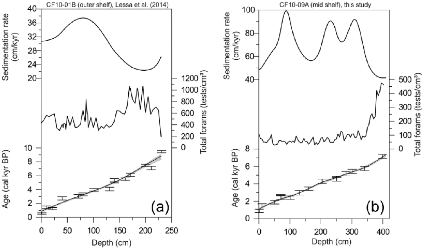
Sedimentation rate, total planktonic foraminiferal density, and geochronological models for the (a) CF10-01B and (b) CF10-09A cores. The gray shading and error bars in the geochronological models represent the 2σ age uncertainty.

The CF10-09A core is considered to be mid-shelf, and the CF10-01B core is treated as outer shelf. The δ¹⁸O of G. ruber (δ¹⁸O_RUB) varied between −1.2‰ and −0.4‰ in the outer shelf and between −1.6‰ and −0.1‰ in the mid-shelf, featuring three main phases in the CFUS: high values in the early and middle Holocene, a transition phase between 5.0 and 4.0 kyr BP, and lower values after 4.0 kyr BP (Figure 3). The δ¹⁸O of G. bulloides (δ¹⁸O_BUL) varied between −0.8‰ and 0‰ in the outer shelf and between −1.1‰ and 0.2‰ in the mid-shelf (Figure 3), with generally higher values than δ¹⁸O_RUB, but one exception was present in the mid-shelf during the middle Holocene (Figure 3). The three stages that were revealed by δ¹⁸O_RUB are only seen in δ¹⁸O_BUL in the mid-shelf, but with an opposite trend in relation to the δ¹⁸O_RUB data. On the outer shelf, no Δδ¹⁸O_{BUL − RUB} trend was observed once the δ¹⁸O_BUL variation did not present a meaningful trend (Figure 3), whereas on the mid-shelf, values that trended toward 0‰ were observed during the early and middle Holocene, with a gradual increase between 5.0 and 4.0 kyr BP (transition phase) and larger differences after 4.0 kyr BP.

Figure 3.

Variation in the Globigerinoides ruber and Globigerina bulloides δ¹⁸O along the CF10-01B (outer shelf) and CF10-09A (mid-shelf) cores. The upper part of the graphic shows the geochemical (gray shading) and foraminiferal assemblage (roman numbers) phases.

The Mg/Ca ratio of G. ruber ranged between 4.0 and 7.0 mmol/mol, with lower values before 5.0 kyr BP and higher values after this age (Figure 4a). The reconstructed temperature (T_Mg/Ca) in the outer shelf from Figure 4b indicated two steps of SST variations that accompanied the variations in the δ¹⁸O_RUB in both studied portions of the continental shelf. Low temperatures were observed between 9.0 and 5.0 kyr BP (variable between 9.0 and 6.5 kyr and stable between 6.5 and 5.0 kyr), followed by high temperatures after 5.0 kyr BP.

Figure 4.

Variation of the Globigerinoides ruber (pink) Mg/Ca and reconstructed paleotemperatures (SST proxy) along the CF10-01B core (outer shelf). Temperature values were forced to CFUS range by subtracting them by a factor of 6.50°C. The gray error bars represent the total uncertainty of reconstruction (i.e. 1.34°C). The upper part of the graphic shows the phases reported by geochemical proxies (gray shading) and the foraminiferal assemblage (roman numbers).

The grouping of the relative abundance of the planktonic foraminifera according to CONISS identified five main stages of assemblage variations during the Holocene (Figure 5). The phases corroborate δ¹⁸O and Mg/Ca results but detail important changes after 5.0 kyr BP that are not perfectly displayed in geochemical records. The relative abundance of G. ruber and G. bulloides changed in opposite fashions throughout the record (Figure 5), except between 9.0 and 4.0 kyr BP in the outer shelf. G. ruber was the most abundant species in the entire record, with a relative abundance that ranged from 35% to 60% (Figure 5). The relative abundance of G. bulloides ranged from 7% to 25%, usually being higher in the mid-shelf compared with the outer shelf. The relative abundance of the G. menardii plexus varied between 0% and 3% and was higher in the outer shelf. The relative abundance of G. sacculifer varied between 0.5% and 5% and was higher in the mid-shelf (Figure 5). The relative abundance of Turborotalita quinqueloba ranged from 2% to 12% and was higher in the mid-shelf during the middle Holocene and in both regions after 1.5 kyr BP. The relative abundance of Globigerinita glutinata ranged between 6% and 20% and was higher in the mid-shelf. The relative abundance of Globoturborotalita rubescens ranged from 8% to 25%, with higher values observed in the outer shelf (Figure 5).

Figure 5.

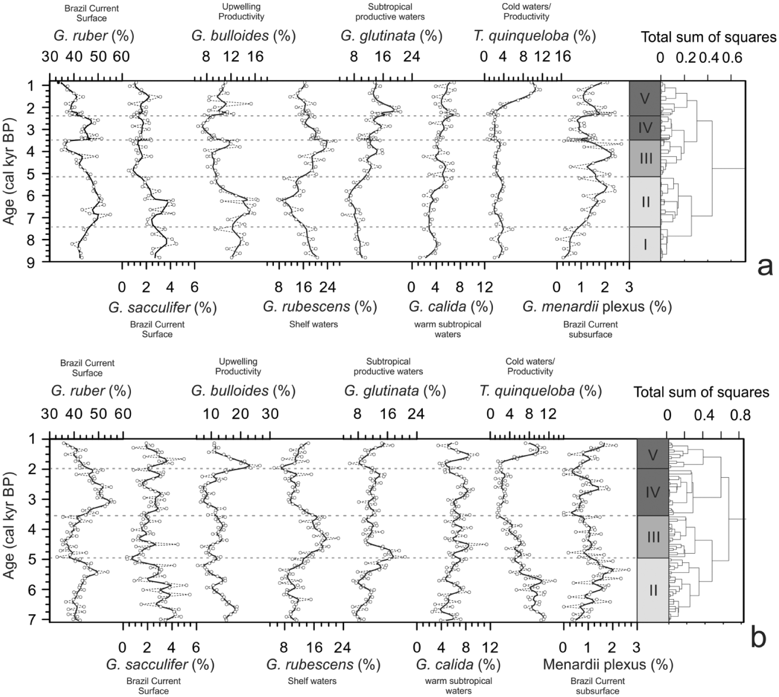
Variation in the relative abundance of main planktonic foraminifera species along the (a) CF10-01B (outer shelf) (modified from Lessa et al., 2014) and (b) CF10-09A (mid-shelf) cores (this study). Only Globigerina bulloides and vertical (age) axis were not scaled to preserve the view of the variations on the outer shelf and mid-shelf high resolution, respectively. The thick lines represent a 5-point smoothing from the raw data. The dashed lines represent the CONISS tree groups, which define the assemblage variation phases. The gray scale shows the correspondence with the δ¹⁸O and Mg/Ca results.

Discussion

BC dynamics during the last 9000 years

Reconstructions that were based on stable isotopes and the Mg/Ca ratio of G. ruber from the CF10-01B core (outer shelf, Figures 4a and 5) reflect primarily variations in the SST of the BC passing the continental margin of Rio de Janeiro (23°S). According to Matano (1993) and Locarnini et al. (2010), changes in the SST of the BC can be positively correlated to the intensity. Belem et al. (2013) through modeling reported intensification of the upwelling with intense BC episodes for the CFUS. These considerations allow us to assume that this relationship may have also been true in the past. A comparison was made between our results for T_Mg/Ca (equivalent to SST) and other records on the western margin of the tropical South Atlantic, including BC and NBC (Figure 6).

Figure 6.

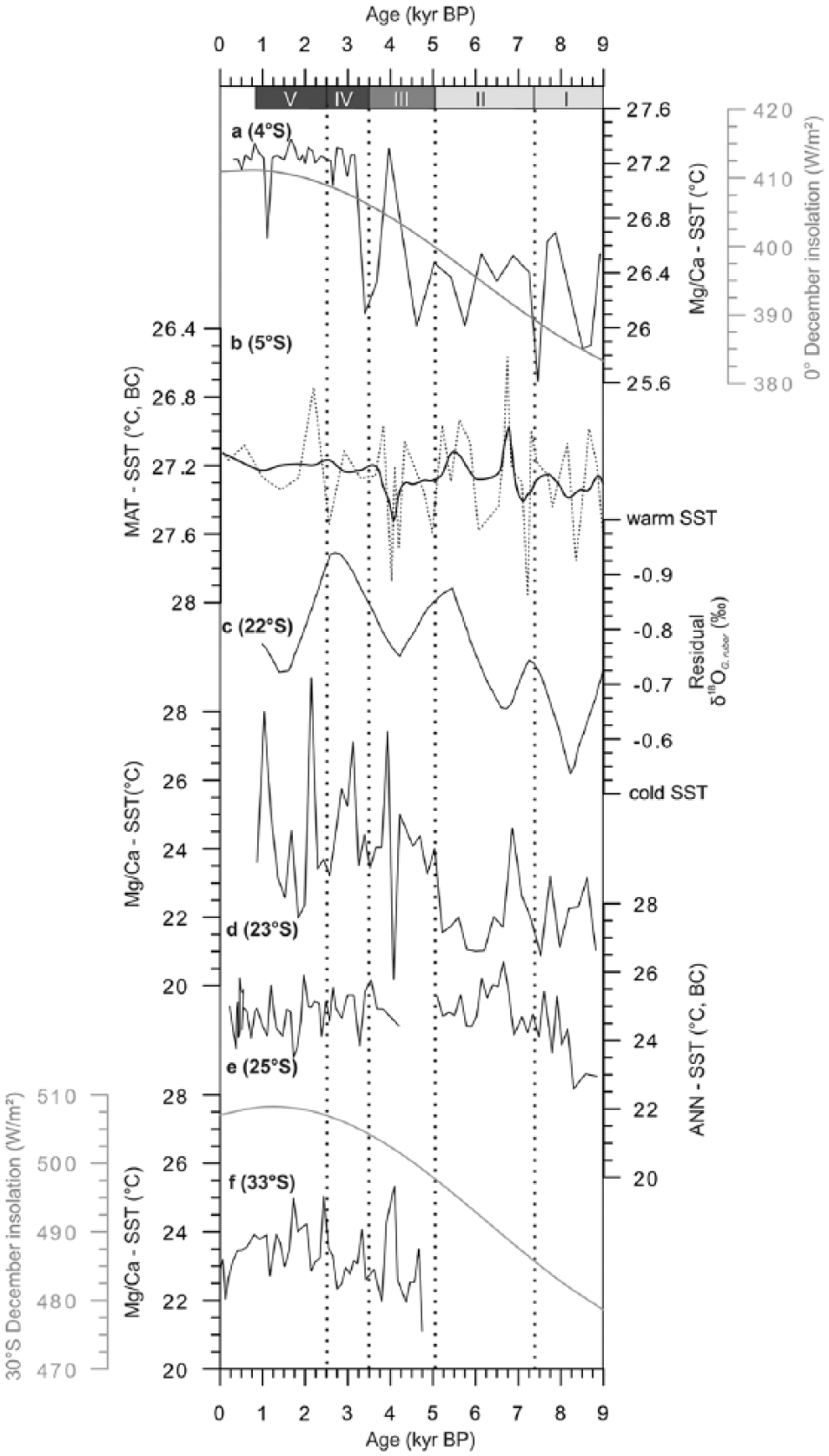
Comparison between equatorial and subtropical southwestern Atlantic SST proxies and December insolation from Berger (1978) during the last 9000 years, with the records placed in latitudinal order: (a) and (b) NBC SST reconstructions from Santos et al. (2013) and Weldeab et al. (2006), respectively; (c) reconstruction of the BC’ SST between 20 and 22°S from Arz et al. (1999); (d) our adjusted Mg/Ca-SST reconstruction from CFUS (23°S); and (e) and (f) SST reconstructions of the BC south of the CFUS by Pivel et al. (2013) and Chiessi et al. (2014), respectively. The five phases are indicated at the top by roman numerals (assemblages), gray scale (geochemical proxies), and vertical dashed lines.

Along the last 9 kyr of the marine records, the SST tended to follow different trends in the NBC and BC domains.

In the NBC domain, a different variation pattern is seen between the Modern Analog Technique (MAT)-SST from Santos et al. (2013) and Mg/Ca-SST from Weldeab et al. (2006) (Figure 6a and b). This difference is probably because the MAT-SST reconstruction includes contributions from surface and subsurface species, whereas the G. ruber Mg/Ca values are linked to the uppermost surface SST. Thus, the two data register SST with different depth length and highlight the importance of the subsurface layer as an indicator of the NBC’s intensity (and therefore of the equatorial sector of the surface AMOC) along the Holocene. The trend change to warmer waters at approximately 4.0 kyr BP (Figure 6c and b, respectively) coincides with the decrease in the AMOC activity in the Sub-Arctic sector (Hall et al., 2004; Kissel et al., 2013; Thornalley et al., 2013). Santos et al.’s (2013) planktonic foraminifera assemblage revealed that the 4.0 kyr BP warming was caused by an increase in subsurface warm and saltier waters species (G. sacculifer, G. menardii plexus, Pulleniatina obliquiloculata, and Neogloboquadrina dutertrei) and a decrease in G. ruber and less abundant warm water species (Globigerinella siphonifera and Globorotalia truncatulinoides). These observations indicate a deeper mixture layer and therefore more heat concentration in the equatorial current system and less export to the North Atlantic.

In the BC domain, an increasing trend is observed from 9.0 to 7.0 kyr BP. Low and stable SST values were observed between 7.0 and 4.5 ± 0.5 kyr BP and high values after 4.0 kyr BP, except at 26°S. Such trends can be best viewed in the low-resolution record of Arz et al. (1999) for the BC at 22°S, which indicates responses to increased summer insolation in the Southern Hemisphere. This pattern would suggest a different behavior of the BC to the north and south of Cabo Frio, but the low resolution of the record in Arz et al. (1999) limits this interpretation. Different BC positions close to or far from the continental shelf break and the stability of the flux may explain the different SST variations that are observed in the subtropical SW Atlantic. Based on these characteristics, we discuss the major phases of the variation in the BC’s dynamics when passing along the continental margin of Rio de Janeiro and how it could have influenced the CFUS. A summary of the scenarios for each phase is found in Table 3, and the CFUS oceanographic model is represented in Figure 7.

Table 3.

Summary of the identified phases in the CFUS along the studied time.

Phase	Time (kyr BP)	Support data	Interpretation
I	9.0–7.0	High abundance of Globigerina bulloides and Globoturborotalita rubescens; low and instable SST and decreasing δ¹⁸O_RUB	Cold and offshore BC because of sea-level and AMOC fluctuations; predominance of cold and shelf waters
II	7.0–5.0	High abundance of Globigerinoides ruber, G. bulloides; contrasted δ¹⁸O_RUB between the mid and outer shelf; strongly variable δ¹⁸O_BUL and low water stratification on the mid-shelf	BC near the outer shelf and intense SACW upwelling events which may have reached the surface layer; probable SPSW contributions
III	5.0–3.5	High SST and δ¹⁸O_RUB (outer shelf), increase in the mid-shelf water stratification; increase in G. rubescens, Globigerinita glutinata	BC more offshore because of the high intensity; influence of the SSW and SACW subsuperficial upwelling
IV	3.5–2.5	Low abundances of G. bulloides and Turborotalita quinqueloba; high abundances of G. ruber and high SST; decreased water stratification	Decrease in the SACW upwelling episodes; predominance of the SSW on the outer shelf and TW on the mid-shelf
V	2.5–0.8	Increase in abundance of G. bulloides, T. quinqueloba and water stratification; reduction in G. ruber	Return of the SACW upwelling and cold shelf waters (Medieval Climatic Anomaly); frequent upwelling events on the mid-shelf

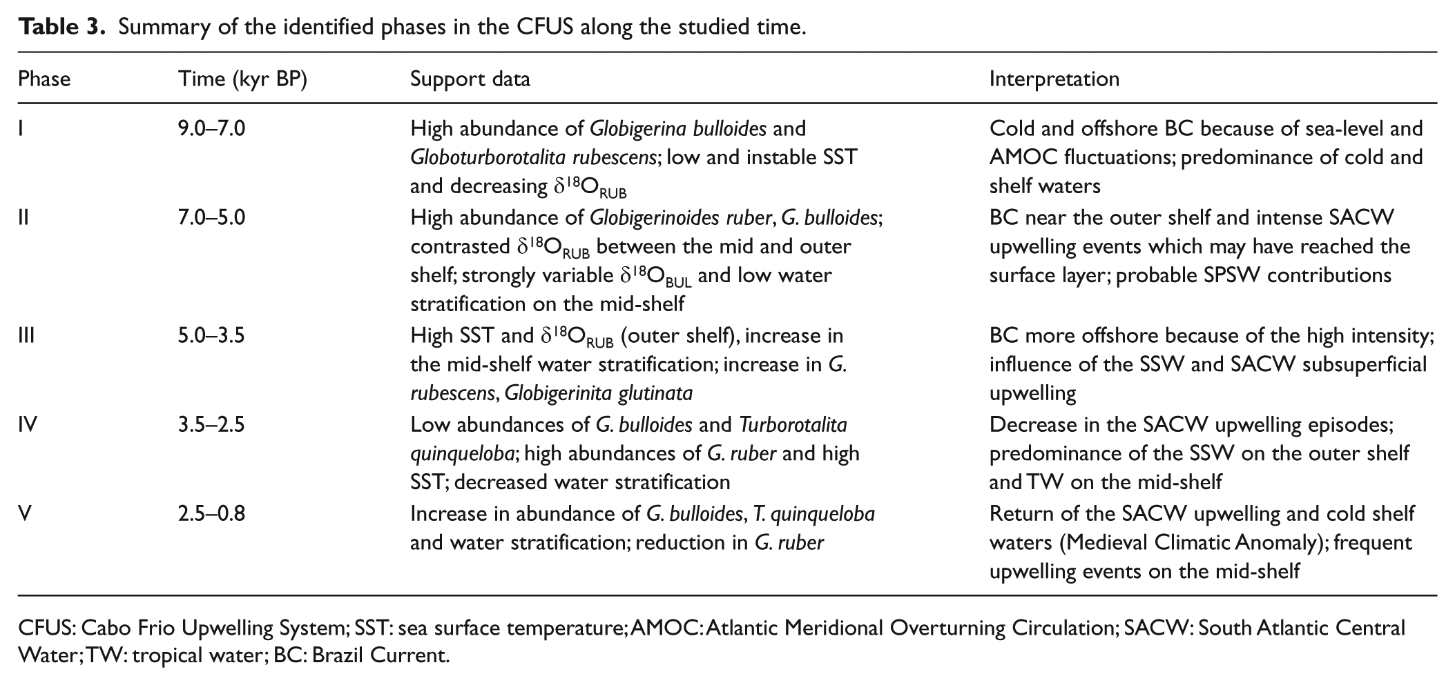
CFUS: Cabo Frio Upwelling System; SST: sea surface temperature; AMOC: Atlantic Meridional Overturning Circulation; SACW: South Atlantic Central Water; TW: tropical water; BC: Brazil Current.

Figure 7.

Main Holocene oceanographic scenarios for the CFUS continental shelf (a–e), which were reconstructed by ecological and geochemical planktonic foraminifera proxies (a–e) represent the described phases I–V, respectively.

Early and middle Holocene

Phase I, which refers to the early Holocene (9.0–7.0 kyr BP, Figure 7a), describes the outer shelf of the CFUS during marine transgression. The high relative abundance of G. bulloides and G. rubescens indicates the influence of cold shelf waters, with little influence of TW on the CFUS. During this phase, the sea level ranged between −45 and 0 m (Corrêa, 1996), indicating that the BC should have been offshore at 9.0 kyr BP, and the BC gradually approached toward the end of the transgressive event (Toledo et al., 2007b). Because of the offshore location of the BC, the influences of the SSW and coastal upwelling plumes were important, influencing the assemblage composition to more cold-water species. In addition, the observed low SST values may be related to a colder BC, where G. ruber is distributed, a consequence of the intensified AMOC during the early Holocene (Arz et al., 1999; Hoogakker et al., 2011; Kissel et al., 2013; Thornalley et al., 2013).

Phase II, which concerns the beginning of the middle Holocene (between 7.2 and 5.0 kyr BP, Figure 7b), was marked by an increase in the influence of TW. The δ¹⁸O_RUB data indicate a gradual approach of the BC because the values are more negative in the outer shelf than in the mid-shelf, but the values follow the same trend over time. The high relative abundance of G. ruber and the G. menardii plexus (Figure 5), combined with the high density of planktonic foraminifera (Figure 2) in both study sites, indicates that there was an increase in the supply of foraminifera from offshore waters to the CFUS, corroborating the approach of the BC that was observed by Lessa et al. (2014) on the outer shelf. The high relative abundance of G. bulloides and T. quinqueloba, with the low abundance of G. glutinata (Figure 5), suggests the occurrence of frequent subsurface upwelling events in both study sites, particularly in the mid-shelf (Figure 5b). Furthermore, the large dispersion of δ¹⁸O_BUL values and the low level of stratification given by Δδ¹⁸O_BUL-RUB (Figure 3) indicate that the nuclei of productivity from the strong upwelling of the SACW may have reached the surface layer in the mid-shelf. The contact between cold subsurface waters and warm surface waters may have contributed to the lower δ¹⁸O_BUL. This pattern indicates that the area with the greatest intensity of upwelling that was driven by the wind stress curl (maximum of mid-shelf upwelling in Figure 1) would be located near the mid-shelf core site, from which the productivity nuclei originated. This evidence characterizes the expected scenario in the middle Holocene for the CFUS without the influence of sea level. In this scenario, the decreased intensity of the BC (explained by a low SST) would be attributed to the high activity of the AMOC, where peaks of NADW production were observed in the NE Sub-Arctic Atlantic between 7.0 and 5.5 kyr BP (Hall et al., 2004; Hoogakker et al., 2011; Kissel et al., 2013; Thornalley et al., 2013).

The SST at 26°S (Figure 6f) remained high between 7.0 and 6.0 kyr BP, whereas the high SST in the CFUS was restricted to a peak at 7.0 kyr BP (Figure 6d). This paradox could be explained by the local BC instabilities near the coast at 23°S (Rio de Janeiro continental margin) because of the bottom topographic structure, which favors SACW upwelling, whereas the more stable flux of the BC at the offshore Santos Basin (26°S) favors the prevalence of warm waters. These warm waters at 26°S could have been contributed from the Agulhas Current to Atlantic Subtropical Gyre and its westward leakages once the 7.0–6.0 kyr SST peak coincided with the G. menardii plexus maximum (Pivel et al., 2013, Figure 4). The relationship between the G. menardii plexus and the Agulhas system is explained by their high abundance in the Indian Ocean and Eastern Tropical Atlantic (Bé, 1977) and their disappearance in the Atlantic during the glacial period (Portilho-Ramos et al., 2014). It suggests that the plexus reached the SW Atlantic sector through the surface AMOC taking advantage of a less ventilated thermocline which characterizes the Agulhas realm (Broecker and Pena, 2014; Sexton and Norris, 2011). However, upwelling indicator species (e.g. G. bulloides and G. glutinata) and species that would help to understand the ANN SST variation (e.g. G. ruber) were not shown in Pivel et al. (2013) (Figure 4), which limits our ability to comprehend the offshore SACW upwelling dynamics. However, results from a core that was sampled on the slope near the Rio de Janeiro continental margin registered variations in the G. menardii plexus and G. bulloides relative abundances (Toledo et al., 2007a) and SST (by MAT) (Toledo et al., 2007b) that seem similar to the CFUS’ variations. However, the Holocene has low resolution, which limits interpretations; therefore, high-resolution studies in this area are necessary.

Transition phase (5.0–3.5 kyr BP)

The post–5 kyr phases can be related to a change in the meridional overturning flow (Figure 6).

Phase III includes the end of the middle Holocene and beginning of the late Holocene (between 5.0 and 3.5 kyr BP; Figure 7c) and is a transition phase when the BC gained intensity and displaced offshore. Thus, the CFUS received more influence from the SSW, and the SACW upwelling was limited to the subsurface. In this phase, the isotopic signatures of the analyzed species differed spatially (Figure 3). The higher reconstructed SST indicated a warmer BC, and the δ¹⁸O of both species tended to diverge in the mid-shelf, indicating a greater stratification of the photic zone, thus isolating the cold water in the subsurface. The increase in the T_Mg/Ca − SST suggests an increase in the intensity of the BC in the CFUS. However, the abrupt increases in the relative abundance of G. glutinata and G. rubescens in the mid-shelf and gradual increases in the outer shelf (Figure 5, Lessa et al., 2014) indicate more contributions from the SSW and therefore the displacing offshore of the BC. Certain aspects of the strong influence from SSW can be addressed as follows.

The time interval of Phase III corresponds to the maximum transgressive event of the Holocene (Angulo et al., 2006), and a possible erosive increase in flooded areas could have enhanced the productivity of the SSW. Likewise, the main habitat of the BC species, such as the G. menardii plexus, tended to approach the CFUS.

Phase III also coincides with a period of great changes in the oceanographic (Figure 6) and continental domains (section ‘Paleoclimate implications’), which were driven by the high summer insolation. At 5.0 kyr BP, the values of δ¹⁸O_RUB decreased in the mid-shelf, while the outer shelf δ¹⁸O values remained high, decreasing only at 4.0 kyr BP, along with the mid-shelf (Figure 3). The similarity between the trends of the SST records of the BC (except at 26°S, Figure 6f) and the NBC (Figure 6b and c) indicates that the increase in the SST of the BC likely responded to the decrease in the AMOC (Andrews et al., 1997; Thornalley et al., 2013), with more heat being distributed toward the BC system.

Late Holocene (after 3.5 kyr BP)

In Phases IV and V (late Holocene), the δ¹⁸O_RUB values acquired their present range, indicating that the BC had reached its modern dynamics, which exhibit an intense flow offshore below 23°S. However, the variations in the relative abundance of cold and warm water species (Figure 5) indicated large local variations in the CFUS. Because oceanographic variations in the BC became stable, upwelling variations in the CFUS were associated with the atmospheric component (NE winds).

Phase IV (between 3.5 and 2.5 kyr BP, Figure 7e) is marked by greatly weakened upwelling. During this period, a higher SST (between 25°C and 27°C, Figure 4) and lower δ¹⁸O_BUL were present in the outer shelf, along with a drop in the relative abundances of cold and productive water species (G. bulloides and T. quinqueloba) and an increase in the relative abundance of G. ruber, G. menardii plexus, and G. glutinata. These results suggest a more frequent prevalence of TW and warm subsurface waters throughout the record in the mid-shelf. Because the NE winds were unable to generate wind stress curl phenomena, shelf waters from the Santos Basin could more easily reach the CFUS, favoring the increase in G. glutinata and G. rubescens, which are abundant in that area (Lessa et al., 2014). Because the zone of the maximum wind stress curl is located in the mid-shelf, the cold-water signature that is given by δ¹⁸O_BUL indicates that the upwelling reached the lower layer of the photic zone, but this phenomenon was rare in the outer shelf, where a decrease in δ¹⁸O_BULwas observed. This situation suggests that G. bulloides, similar to the biota that adapted to the productivity of the upwelling, migrated to the deeper layers in the photic zone (Bé, 1960; Peeters et al., 2002). Considering that the relative abundances of species in the mid-shelf that were linked to the BC increased (Figure 5b), the incursions of TW could have resulted in the deepening of the photic zone through increased transparency. This deepening may not have occurred in the outer shelf, which remained more strongly influenced by SSW (richer in nutrients than TW) than the mid-shelf.

Phase V, which corresponds to the interval 2.5–0.8 kyr BP (Figure 7f), marks the establishment of the current CFUS oceanographic configuration. The increase in the relative abundance of species from cold and productive waters (G. bulloides and T. quinqueloba) in the outer shelf and mid-shelf at 2.5 and 2.1 kyr BP, respectively, indicated a gradual return of SACW intrusion into the platform. However, G. bulloides and T. quinqueloba tended to vary in opposite ways, suggesting a competition between the two species. The periods between 2.5 and 1.5 kyr BP and between 1.5 and 0.8 kyr BP were marked by an increase in G. bulloides and T. quinqueloba, respectively. These changes could be associated with variations in salinity because T. quinqueloba prefers lower salinities than G. bulloides (Tolderlund and Be, 1971). The differences between the associations of both species are discussed in greater detail in section ‘Influence of subpolar shelf waters in the middle Holocene and Medieval Climatic Anomaly’.

Paleoclimate implications

Atlantic and South American atmospheric teleconnections

Changes in oceanographic and atmospheric conditions were observed at the end of the middle Holocene (±5.0 kyr BP) within the Atlantic Ocean (Figure 6) and along the South American and African continents (Cruz et al., 2009; DeMenocal et al., 2000). These changes coincide with the start of Phase III (5.0–3.5 kyr BP), when an oceanographic transition toward the present configuration of the CFUS began (Figures 4 and 5). The reconstructions of atmospheric systems indicated a change in the hydrological regime along the African and South American continents at approximately 5.0 kyr BP. The mid-Holocene was marked by a humid climate in the Sahara and NE Brazil (Cruz et al., 2009; DeMenocal et al., 2000), while the climate in the Amazon was dry, with high records of pollen from savanna grasses and micro-charcoals from fires (Absy et al., 1991). These studies have linked such climatic conditions to the Intertropical Convergence Zone (ITCZ), which distributed moisture before 5.0 kyr BP and therefore was not frequent in the Amazon (Cruz et al., 2009; Haug et al., 2001). The period of wide ITCZ migration coincides with Phase II of the CFUS and may suggest a seasonal extreme intensification, but higher resolution data would be required for a more rigorous confirmation. Such atmospheric conditions also suggest that the SE region of Brazil also featured a drier climate, as the decreased moisture in the Amazon in the middle Holocene prevented and/or deflected the formation of a humidity corridor from the SACZ in the summer because of the greater intensity of the South Atlantic Subtropical High (SASH).

The shorter ITCZ seasonal migration after 5.0 kyr BP (in average displaced to the south) favored the desertification of the Sahara (DeMenocal et al., 2000) and allowed the expansion of the semiarid climate in NE Brazil (Cruz et al., 2009). This pattern favored the increased presence of low-pressure areas over the Amazon, causing the intensification of the South American monsoon and expanding the tropical rainforest vegetation (Absy et al., 1991; Cordeiro et al., 2008; Cruz et al., 2009; Sifeddine et al., 2001; Turcq et al., 2002). Thus, an increase in the rainforest caused a rise in humidity, allowing the formation and intensification of the SACZ. Therefore, the climate that was dry in the CFUS region before 5.0 kyr BP (Laslandes et al., 2006) became humid after 4.5 kyr BP, indicating that this factor may have contributed to the advancement of the SSW into the CFUS, as mentioned in section ‘Brazil Current dynamics during the last 9000 years’. After 5.0 kyr BP, the upwelling in the CFUS became limited to the subsurface (Figure 3), indicating that the zone of the maximum wind stress curl shifted away, causing upwelling episodes in the SACW to be barely evident in the outer shelf, as shown by the assemblage and δ¹⁸Odata (Figures 3 and 6). The high SST in the SW Subtropical Atlantic also suggests a strengthening of the oceanic component of the SACZ because this component tends to intensify during episodes of high SST (Prado et al., 2013), suggesting that the climate in SE Brazil became humid. Since Prado et al. (2013) emphasized that the SST decreased because of the formation of an oceanic SACZ, such an event could have been most intense between 25°S and 23°S, as shown in Figure 6.

Influence of SPSWs in the middle Holocene and Medieval Climatic Anomaly

The occurrence of SPSW in the CFUS during the winter is supported by the atmospheric conditions that were described in Piola et al. (2008). The weakening of subtropical atmospheric systems allows the intrusion of subpolar atmospheric systems, such as cold fronts (associated with SW winds). An increased frequency of SW winds displaces SPSFs northward, currently making the SPSW reach 25°S in the winter, as mentioned previously. Despite the loss of the physical and chemical characteristics of the mid-shelf because of river or lake discharges, organisms that had adapted to cold waters could survive and settle in favorable locations. The CFUS favors the establishment of these species because of the occurrence of a shallow thermocline. Thus, the SPSW could have influenced the present and past communities in the subsurface water column and sediment of the CFUS.

A high relative abundance of T. quinqueloba, either occurring alone or in association with G. bulloides (Figure 5), could reflect an influence of SPSW once other studies have also shown abundant species of the Malvinas Current at 23°S (Stevenson et al., 1998). As mentioned in section ‘Brazil Current dynamics during the last 9000 years’, the replacement of G. bulloides by T. quinqueloba in the assemblage can occur with a decrease in the salinity of cold waters. This pattern can reinforce the idea of possible penetrations by SPSW. A higher relative abundance of T. quinqueloba in our study area (Figure 5) occurs during Phase II (7.0–5.0 kyr BP) in the mid-shelf and after 1.8 kyr BP throughout the CFUS, with the maximum occurring at approximately 1.0 kyr BP, which corresponds to the Medieval Climate Anomaly (MCA). This interpretation suggests that an event that was associated with the middle Holocene was repeated during the MCA on a larger scale because other studies (Lessa et al., 2014; Souto et al., 2011) showed a higher relative abundance of T. quinqueloba from 1.8 kyr BP, with a maximum abundance during the MCA. Based on the climatic and oceanographic conditions, both Phase II (middle Holocene) and the MCA were marked by frequent passages of cold fronts in the winter. During Phase II, the passages may have occurred because of the northward migration of polar atmospheric systems from weaker insolation. During the MCA, the increase in cold fronts could be explained by La Niña–like conditions (Makou et al., 2010) that favored cold fronts to pass rapidly through the region and often reach latitudes as low as 10°S on the Brazilian coast.

NE winds weakening between 3.5 and 2.5 kyr BP

The return of cold water from the SACW, which was observed after 4.0 kyr BP, is supported by other studies that were conducted in the region (Laslandes et al., 2006; Mahiques et al., 2005; Nagai et al., 2009; Sylvestre et al., 2005). During this period, high SSTs were present along the western edge of the South Atlantic (Figure 7), thus strengthening the subtropical gyre and associated weather systems (Kim and Schneider, 2003). Conditions for weakening SACW intrusions into the CFUS between 3.5 and 2.5 kyr BP are not clear in records outside of the CFUS, which indicate a very active BC (favorable for intrusions by SACW). One possible explanation would be a decrease in the occurrence of NE winds, causing the subtropical waters of the Santos Basin to be more common during this stage, given the high relative abundance of G. rubescens, G. glutinata, and G. ruber. The passage of shelf waters from the SSW in the outer shelf would serve as a barrier to SACW entry and help transport TW to the mid-shelf through the meandering BC. The presence of particulate-free TW in the mid-shelf could also have facilitated the maintenance of a degree of productivity at greater depths because the TW may have allowed a lower layer of the photic zone to reach areas under the influence of the SACW (Figure 3, δ¹⁸O_BUL). Braconnot et al. (2007) showed changes in wind patterns at low atmospheric levels after 3.0 kyr BP through global modeling, which indicate the reintensification of NE winds after 3.0 kyr BP because of a southward shift of the ITCZ. This displacement of the ITCZ favored the approaching and intensification of the Subtropical South Atlantic high-pressure system intensifying the NE winds and promoting the return of SACW intrusions (Phase V) into the CFUS.

Conclusion

Oxygen stable isotopes, Mg/Ca ratio, and assemblage records of planktonic foraminifera assisted in the paleoceanographic reconstruction of the CFUS during the Holocene, during which five main phases were summarized. The first phase (9.0–7.0 kyr BP) was influenced primarily by sea-level variations, which kept the BC away from our study area. The second phase (7.0–5.0 kyr BP) was influenced by a relatively wide BC migration onshore and offshore, favoring the alternation of strong upwelling, the possible influence of SPSW, and the strong presence of TW. The third phase (5.0–3.5 kyr BP) was influenced by oceanographic and climatic transitions from the middle Holocene to late Holocene, during which an intensification of the BC front caused its offshore displacement, favoring a greater SSW influence and the restriction of SACW upwelling to subsurface layers. The fourth (3.5–2.5 kyr BP) and fifth phases (after 2.5 kyr BP) were basically influenced by weak and intense NE winds, respectively. Low (High) intensity of the NE winds was responsible for the prevalence of TW and SSW (SACW upwelling) in the fourth (fifth) phase. Regional and global events were identified by our indicators, such as the transitions between phases II and III (5.0 kyr BP), which are connected with reduced strength of AMOC and the high influence of SPSW during the MCA (approximately 1.0 kyr BP).

Footnotes

Acknowledgements

We also thank LMI PALEOTRACES from Institut de Recherche pour le Développement (IRD, France) and the valuable analytical assistance of Florence le Cornec and Magloire Mandeng-Yogo. D Lessa and ALS Albuquerque were PhD scholar and senior scholar, respectively, from Conselho Nacional de Desenvolvimento Científico e Tecnológico-CNPq (Grant 306385/2013-9). The authors thank Catia Fernandes Barbosa and Rodrigo Portilho-Ramos for their contributions in the identification of planktonic foraminifera species, ecological remarks, and picking of tests for geochemical analysis. We also thank Aline Govin and an anonymous reviewer for their contributions, which improved the manuscript.

Funding

This study was partially funded by Coordenação de Aperfeiçoamento de Pessoal de Nível Superior (CAPES) through the Projeto PALEOCEANO (Grant: 23038.00141/2014-71), the Geochemistry Network from PETROBRAS/CENPES, and the National Petroleum Agency (ANP) of Brazil (Grant 0050.004388.08.9).

References

Absy

Cleef

Fournier

. (1991) Mise en évidence de quatre phases d’ouverture de la forêt dense dans le sud-est de l’Amazonie au cours des 60 000 dernières années. Première comparaison avec d’autres régions tropicales. Paris: Gauthier-Villars.

Aguiar

Cirano

Pereira

. (2014) Upwelling processes along a western boundary current in the Abrolhos–Campos region of Brazil. Continental Shelf Research 85: 42–59.

Albuquerque

ALS

Belem

Zuluaga

FJB

. (2014) Particle fluxes and bulk geochemical characterization of the Cabo Frio upwelling system in Southeastern Brazil: Sediment trap experiments between Spring 2010 and Summer 2012. Anais da Academia Brasileira de Ciências 86: 601–620.

Anand

Elderfield

Conte

(2003) Calibration of Mg/Ca thermometry in planktonic foraminifera from a sediment trap time series. Paleoceanography 18: 1050.

Andrews

Smith

Preston

. (1997) Spatial and temporal patterns of iceberg rafting (IRD) along the East Greenland margin, ca. 68°N, over the last 14 cal.kyr. Journal of Quaternary Science 12: 1–13.

Angulo

de Souza

Reimer

. (2005) Reservoir effect of the southern and southeastern Brazilian coast. Radiocarbon 47: 1–7.

Angulo

Lessa

Souza

(2006) A critical review of mid-to late-Holocene sea-level fluctuations on the eastern Brazilian coastline. Quaternary Science Reviews 25(5): 486–506.

Arz

Pätzold

Wefer

(1999) The deglacial history of the western tropical Atlantic as inferred from high resolution stable isotope records off northeastern Brazil. Earth and Planetary Science Letters 167: 105–117.

Barker

Greaves

Elderfield

(2003) A study of cleaning procedures used for foraminiferal Mg/Ca paleothermometry. Geochemistry, Geophysics, Geosystems 4: 8407.

10.

Bé

AWH

(1960) Ecology of Recent planktonic foraminifera-Part 2, Bathymetric and seasonal distributions in the Sargasso Sea off Bermuda. Micropaleontology 6(4): 373–392.

11.

Bé

AWH

(1977) An ecological, zoogeographic and taxonomic review of recent planktonic foraminifera. In: Ramsay

ATS

(ed.) Oceanic Micropaleontology. London: Academic Press, pp. 1–100.

12.

Belem

Castelao

Albuquerque

(2013) Controls of subsurface temperature variability in a western boundary upwelling system. Geophysical Research Letters 40: 1362–1366.

13.

Berger (1978) Long-term variations of daily insolation and Quaternary climatic changes. Journal of the Atmospheric Sciences 35: 2362–2367.

14.

Bergue

Coimbra

Cronin

(2007) Cytherellid species (Ostracoda) and their significance to the Late Quaternary events in the Santos Basin, Brazil. Senckenbergiana maritima 37: 5–12.

15.

Blaauw

(2010) Methods and code for ‘classical’ age-modeling of radiocarbon sequences. Quaternary Geochronology 5: 512–518.

16.

Braconnot

Otto-Bliesner

Harrison

. (2007) Results of PMIP2 coupled simulations of the Mid-Holocene and Last Glacial Maximum – Part 2: Feedbacks with emphasis on the location of the ITCZ and mid- and high latitudes heat budget. Climate of the Past 3: 279–296.

17.

Broecker

Pena

(2014) Delayed Holocene reappearance of G. menardii. Paleoceanography 29(4): 291–295.

18.

Calado

da Silveira

ICA

Gangopadhyay

. (2010) Eddy-induced upwelling off Cape São Tomé (22°S, Brazil). Continental Shelf Research 30: 1181–1188.

19.

Campos

EJD

Velhote

da Silveira

ICA

(2000) Shelf break upwelling driven by Brazil Current Cyclonic Meanders. Geophysical Research Letters 27: 751–754.

20.

Campos

Möller

Piola

. (2013) Seasonal variability and coastal upwelling near Cape Santa Marta (Brazil). Journal of Geophysical Research: Oceans 118: 1420–1433.

21.

Carvalho

LMV

Jones

Liebmann

(2004) The South Atlantic Convergence Zone: Intensity, form, persistence, and relationships with intraseasonal to interannual activity and extreme rainfall. Journal of Climate 17: 88–108.

22.

Castelao

Barth

(2006) Upwelling around Cabo Frio, Brazil: The importance of wind stress curl. Geophysical Research Letters 33: L03602.

23.

Cerda

Castro

(2014) Hydrographic climatology of South Brazil Bight shelf waters between Sao Sebastiao (24°S) and Cabo Sao Tome (22°S). Continental Shelf Research 89: 5–14.

24.

Chaves

Nobre

(2004) Interactions between sea surface temperature over the South Atlantic Ocean and the South Atlantic Convergence Zone. Geophysical Research Letters 31: L03204.

25.

Chiessi

Mulitza

Groeneveld

. (2014) Variability of the Brazil Current during the late Holocene. Palaeogeography, Palaeoclimatology, Palaeoecology 415: 28–36.

26.

Chiessi

Mulitza

Mollenhauer

. (2015) Thermal evolution of the western South Atlantic and the adjacent continent during Termination 1. Climate of the Past 11(6): 915–929.

27.

Cordeiro

Turcq

Suguio

. (2008) Holocene fires in East Amazonia (Carajás), new evidences, chronology and relation with paleoclimate. Global and Planetary Change 61: 49–62.

28.

Corrêa

ICS

(1996) Les variations du niveau de la mer durant les derniers 17.500 ans BP: L’exemple de la plate-forme continentale du Rio Grande do Sul-Bésill. Marine Geology 130: 163–178.

29.

Cruz

Vuille

Burns

. (2009) Orbitally driven east-west antiphasing of South American precipitation. Nature Geoscience 2: 210–214.

30.

Delworth

Zeng

(2012) Multicentennial variability of the Atlantic meridional overturning circulation and its climatic influence in a 4000 year simulation of the GFDL CM2. 1 climate model. Geophysical Research Letters 39(13): L13702.

31.

DeMenocal

Ortiz

Guilderson

. (2000) Abrupt onset and termination of the African Humid Period: Rapid climate responses to gradual insolation forcing. Quaternary Science Reviews 19: 347–361.

32.

Ericson

Wollin

(1968) Pleistocene climates and chronology in deep-sea sediments. Science 162: 1227–1234.

33.

Grimm

(1987) CONISS: A FORTRAN 77 program for stratigraphically constrained cluster analysis by the method of incremental sum of squares. Computers & Geosciences 13: 13–35.

34.

Hall

Bianchi

Evans

(2004) Centennial to millennial scale Holocene climate-deep water linkage in the North Atlantic. Quaternary Science Reviews 23: 1529–1536.

35.

Haug

Hughen

KYR

Sigman

. (2001) Southward migration of the Intertropical Convergence Zone through the Holocene. Science 293: 1304–1308.

36.

Hoogakker

BAA

Chapman

McCave

. (2011) Dynamics of North Atlantic Deep Water masses during the Holocene. Paleoceanography 26: PA4214.

37.

Kim

Schneider

(2003) Low-latitude control of interhemispheric sea-surface temperature contrast in the tropical Atlantic over the past 21 kyears: The possible role of SE trade winds. Climate Dynamics 21: 337–347.

38.

Kissel

Van Toer

Laj

. (2013) Variations in the strength of the North Atlantic bottom water during Holocene. Earth and Planetary Science Letters 369–370: 248–259.

39.

Kuhlbrodt

Griesel

Montoya

. (2007) On the driving processes of the Atlantic meridional overturning circulation. Reviews of Geophysics 45(2): 1–32.

40.

Laslandes

Sylvestre

Sifeddine

. (2006) Enregistrement de la variabilité hydroclimatique au cours des 6500 dernières années sur le littoral de Cabo Frio (Rio de Janeiro, Brésil). Comptes Rendus Geoscience 338: 667–675.

41.

Lessa

DVO

Portilho-Ramos

Barbosa

. (2014) Planktonic foraminifera in the sediment of a western boundary upwelling system off Cabo Frio, Brazil. Marine Micropaleontology 106: 55–68.

42.

Locarnini

Mishonov

Antonov

. (2010) World Ocean Atlas 2009, Vol. 1: Temperature. In: Levitus

(ed.) NOAA Atlas NESDIS 68. Washington, DC: U.S. Government Printing Office, pp. 1–40.

43.

Loeblich

Tappan

(1988) Foraminiferal Genera and Their Classification. New York: Van Nostrand Reinhold.

44.

Mahiques

Bícego

Silveira

ICA

. (2005) Modern sedimentation in the Cabo Frio upwelling system, Southeastern Brazilian shelf. Anais da Academia Brasileira de Ciências 77: 535–548.

45.

Mahiques

Tessler

Maria Ciotti

. (2004) Hydrodynamically driven patterns of recent sedimentation in the shelf and upper slope off Southeast Brazil. Continental Shelf Research 24: 1685–1697.

46.

Makou

Eglinton

Oppo

. (2010) Postglacial changes in El Niño and La Niña behavior. Geology 38: 43–46.

47.

MARGO (2009) Constraints on the magnitude and patterns of ocean cooling at the last glacial maximum. Nature Geoscience 2(2): 127–132.

48.

Matano

(1993) On the separation of the Brazil Current from the Coast. Journal of Physical Oceanography 23: 79–90.

49.

Mendoza

Neto

Abuchacra

. (2014) Geoacoustic character, sedimentology and chronology of a cross-shelf Holocene sediment deposit off Cabo Frio, Brazil (southwest Atlantic Ocean). Geo-Marine Letters 34: 297–314.

50.

Nagai

Sousa

SHM

Burone

. (2009) Paleoproductivity changes during the Holocene in the inner shelf of Cabo Frio, southeastern Brazilian continental margin: Benthic foraminifera and sedimentological proxies. Quaternary International 206: 62–71.

51.

Peeters

Brummer

GJA

Ganssen

(2002) The effect of upwelling on the distribution and stable isotope composition of Globigerina bulloides and Globigerinoides ruber (planktic foraminifera) in modern surface waters of the NW Arabian Sea. Global and Planetary Change 34(3): 269–291.

52.

Peterson

Stramma

(1991) Upper-level circulation in the South Atlantic Ocean. Progress in Oceanography 26: 1–73.

53.

Pierre

Vergnaud-Grazzini

Faugères

(1991) Oxygen and carbon stable isotope tracers of the water masses in the Central Brazil Basin. Deep Sea Research, Part A: Oceanographic Research Papers 38(5): 597–606.

54.

Piola

Campos

EJD

Möller

. (2000) Subtropical Shelf Front off eastern South America. Journal of Geophysical Research: Oceans 105: 6565–6578.

55.

Piola

Möller

Guerrero

. (2008) Variability of the subtropical shelf front off eastern South America: Winter 2003 and summer 2004. Continental Shelf Research 28(13): 1639–1648.

56.

Pivel

MAG

Santarosa

ACA

Toledo

FAL

. (2013) The Holocene onset in the southwestern South Atlantic. Palaeogeography, Palaeoclimatology, Palaeoecology 374: 164–172.

57.

Portilho-Ramos

Barbosa

Rios-Netto

(2014) Planktonic foraminiferal variations in the Southwestern Atlantic since the last glacial–interglacial cycle. Palaios 29(1): 38–44.

58.

Prado

Wainer

Chiessi

. (2013) Mid-Holocene climate reconstruction for eastern South America. Climate of the Past 9: 2117–2133.

59.

Reimer

Baillie

MGL

Bard

. (2009) IntCal09 and Marine09 radiocarbon age calibration curves, 0–50,000 years cal BP. Radiocarbon 51(4): 1111–1150.

60.

Robertson

Mechoso

(2000) Interannual and interdecadal variability of the South Atlantic Convergence Zone. Monthly Weather Review 128: 2947–2957.

61.

Rodrigues

Lorenzzetti

(2001) A numerical study of the effects of bottom topography and coastline geometry on the Southeast Brazilian coastal upwelling. Continental Shelf Research 21: 371–394.

62.

Santos

Franco

Barbosa

. (2013) Millennial- to centennial-scale changes in sea surface temperature in the tropical South Atlantic throughout the Holocene. Palaeogeography, Palaeoclimatology, Palaeoecology 392: 1–8.

63.

Sexton

Norris

(2011) High latitude regulation of low latitude thermocline ventilation and planktic foraminifer populations across glacial–interglacial cycles. Earth and Planetary Science Letters 311(1): 69–81.

64.

Sifeddine

Martin

Turcq

. (2001) Variations of the Amazonian rainforest environment: A sedimentological record covering 30,000 years. Palaeogeography, Palaeoclimatology, Palaeoecology 168: 221–235.

65.

Silveira

ICA

Schmidt

ACK

Campos

EJD

. (2000) A corrente do Brasil ao largo da costa leste brasileira. Revista Brasileira de Oceanografia 48: 171–183.

66.

Souto

Lessa

Albuquerque

ALS

. (2011) Marine sediments from southeastern Brazilian continental shelf: A 1200 year record of upwelling productivity. Palaeogeography, Palaeoclimatology, Palaeoecology 299(1): 49–55.

67.

Stevenson

Dias-Brito

Stech

. (1998) How do cold water biota arrive in a tropical bay near Rio de Janeiro, Brazil? Continental Shelf Research 18: 1595–1612.

68.

Stramma

England

(1999) On the water masses and mean circulation of the South Atlantic Ocean. Journal of Geophysical Research 104: 20863–20883.

69.

Sylvestre

Sifeddine

Turcq

. (2005) Hydrological changes related to the variability of tropical South American climate from the Cabo Frio lagoonal system (Brazil) during the last 5000 years. The Holocene 15: 625–630.

70.

Thornalley

DJR

Blaschek

Davies

. (2013) Long-term variations in Iceland-Scotland overflow strength during the Holocene. Climate of the Past 9: 2073–2084.

71.

Tolderlund

AWH

(1971) Seasonal distribution of planktonic foraminifera in the western North Atlantic. Micropaleontology 17: 297–329.

72.

Toledo

Costa

Pivel

. (2008) Tracing past circulation changes in the western South Atlantic based on planktonic foraminifera. Revista Brasileira de Paleontologia 11: 169–178.

73.

Toledo

FAL

Cachão

Costa

. (2007a) Planktonic foraminifera, calcareous nanoplankton and ascidian variations during the last 25 kyr in the Southwestern Atlantic: A paleoproductivity signature? Marine Micropaleontology 64: 67–79.

74.

Toledo

FAL

Costa

Pivel

MAG

(2007b) Salinity changes in the western tropical South Atlantic during the last 30 kyr. Global and Planetary Change 57: 383–395.

75.

Turcq

Albuquerque

ALS

Cordeiro

. (2002) Accumulation of organic carbon in five Brazilian lakes during the Holocene. Sedimentary Geology 148: 319–342.

76.

Valentin

(1984) Analyse des paramètres hydrobiologiques dans la remontée de Cabo Frio (Brésil). Marine Biology 82: 259–276.

77.

Venâncio

Belem

dos Santos

THR

. (2014) Influence of continental shelf processes in the water mass balance and productivity from stable isotope data on the Southeastern Brazilian coast. Journal of Marine Systems 139: 241–247.

78.

Weldeab

Schneider

Kölling

(2006) Deglacial sea surface temperature and salinity increase in the western tropical Atlantic in synchrony with high latitude climate instabilities. Earth and Planetary Science Letters 241(3): 699–706.

79.

Yoshinaga

Sumida

Wakeham

(2008) Lipid biomarkers in surface sediments from an unusual coastal upwelling area from the SW Atlantic Ocean. Organic Geochemistry 39(10): 1385–1399.