
Abstract
Uninterrupted, annually resolved paleoclimate records are crucial to contextualize the current global change. Such information is particularly relevant for the Europe realm for which weather and climate projections are still very challenging if not virtually impossible. This study presents the first precisely dated, annually resolved, multiregional Arctica islandica chronologies from the North Sea which cover the time interval
Keywords
Introduction
Uninterrupted, long-term, high-resolution paleoenvironmental proxy data provide an essential means to test and verify numerical climate models (IPCC, 2007; Jones et al., 2001, 2009) and contextualize present climate change. Such data are particularly relevant for Europe and adjacent marine settings for which weather and climate predictions beyond timescales of several days are virtually impossible at present (Woollings, 2010). The difficulty to predict future change in this region results from (1) the dynamic and non-stationary behavior of oceanic and atmospheric circulation patterns that govern European climate (Greatbatch, 2000), that is, the Atlantic Meridional Overturning Circulation (AMOC; Delworth and Mann, 2000; Schlesinger and Ramankutty, 1994; Wei et al., 2012) and the North Atlantic Oscillation (NAO; Hurrell, 1995; Van Loon and Rogers, 1978) and (2) the lack of sufficient long-term, high-resolution paleoclimate datasets.
Numerous terrestrial, annually resolved paleoclimate archives (e.g. tree rings – Briffa et al., 1992; Esper et al., 2002; Grudd et al., 2002; stalagmites – Fohlmeister et al., 2012; Scholz et al., 2012; Vollweiler et al., 2006; varved lake sediments – Sirocko et al., 2012) spanning centuries to millennia have yielded unique insights into the European climate history and highlighted potential links to cultural transformations (Büntgen et al., 2012). However, one major drawback of these records is that they tend to be biased toward summer, whereas environmental variables during other seasons are only indirectly recorded. Furthermore, a more detailed understanding of the European climate also requires knowledge of environmental variability in adjacent oceans, specifically the North Sea, which exerts a direct influence on climate of the littoral states.
As demonstrated by several recent studies, shells of long-lived bivalve mollusks, in particular the ocean quahog, Arctica islandica, contain detailed records of decadal to century-scale environmental change in the northern North Atlantic (Schöne et al., 2003; Wanamaker et al., 2012; Witbaard et al., 1997). Based on synchronous changes in shell growth and a common response to environmental fluctuations, increment width time-series of specimens with overlapping life spans can be combined by means of cross-dating (wiggle-matching) into single composite or master chronologies (Butler et al., 2010; Marchitto et al., 2000; Schöne et al., 2003; Thompson et al., 1980; Witbaard et al., 1997). This time-series can cover centuries to millennia, including many generations of bivalves and provide information on common environmental variables that influenced the growth of all studied specimens. Furthermore, these chronologies serve as a framework to place geochemical proxy data, for example, stable oxygen and carbon isotope values or trace element data of the shells into a precise temporal context (Schöne et al., 2005b, 2011; Wanamaker et al., 2012).
Here, we present the first millennial-scale A. islandica chronologies from the North Sea. Our study mainly addresses the following questions: Which quasi-decadal and multi-decadal variability is recorded by the shells? Is the relative strength of these oscillations changing through time and why? Which environmental variables are recorded by the shells? Results of our study can be used to better understand the climate history in the northeast Atlantic realm and help to better constrain numerical climate models.
Material and methods
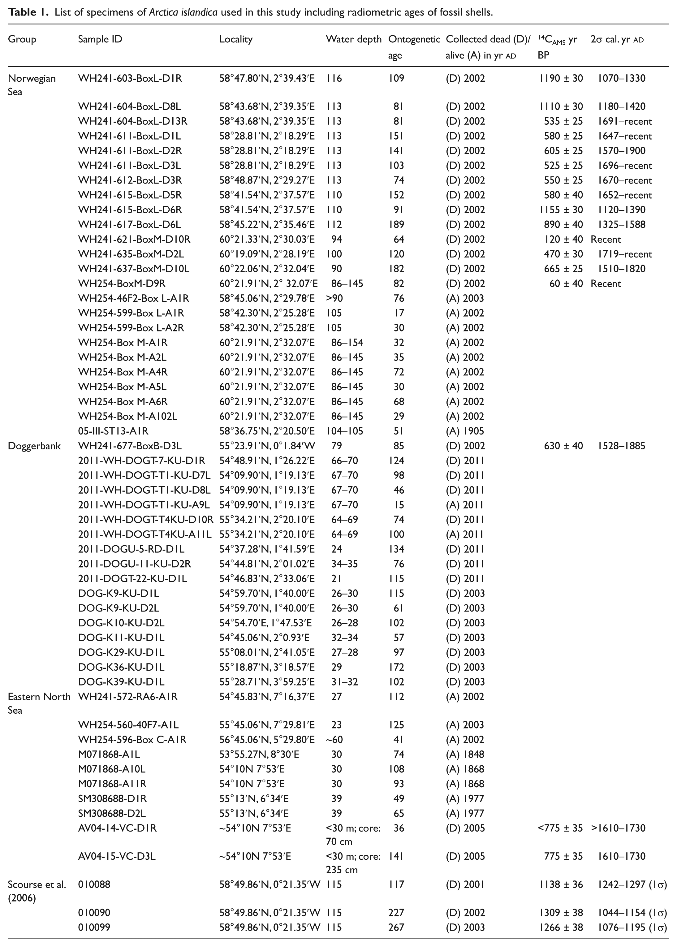
A total of 51 shells of A. islandica were obtained from several localities of the North Sea by means of bottom trawling and ring-dredge fishing (Figure 1, Table 1). All studied specimens lived below the thermocline between c. 20 and 115 m water depth. In all, 31 specimens were well-preserved fossils without external signs of erosion or diagenesis. Even the periostracum, which is prone to quick decay after death, was well preserved. The remaining individuals were collected alive. Three additional time-series taken from the floating chronology of Scourse et al. (2006) were combined with our chronologies in order to increase the sample depth (number of specimens per time interval).

Map showing sampling regions of Arctica islandica in the North Sea and major currents. Map based on Turrell (1992) and Turrell et al. (1992). Not included are the Fladen Ground specimens of the study by Scourse et al. (2006). Shells are divided into three groups: Norwegian Sea (upper box), Doggerbank (left box), and Eastern North Sea (right boxes). For a detailed list of samples, see Table 1.
List of specimens of Arctica islandica used in this study including radiometric ages of fossil shells.
Radiocarbon dating
In order to place the fossil shells in a temporal context, 16 specimens were dated by means of 14CAMS (Table 1). For this purpose, 70–100 mg of carbonate powder was milled from the umbonal shell portions covering c. 6 years of growth. Samples were analyzed by the Poznań Radiocarbon Laboratory, Poland. Radiocarbon dates (Libby years) were subsequently calibrated with the software tool CALIB 5.0.2 (http://calib.qub.ac.uk/calib/), assuming published marine reservoir correction (ΔR) values of 20 ± 42 and 14 ± 55 years (Harkness, 1983; Mangerud and Gulliksen, 1975), respectively. Datasets for the calibration are based on Stuiver et al. (1998) and Hughen et al. (2004).
Shell preparation and sclerochronological measurements
In preparation for shell growth pattern analysis, clean shells were mounted on Plexiglas cubes with a plastic welder (GlueTec Multipower). To avoid fractures during the sawing, a fast drying, two-component metal epoxy resin (WIKO Flüssigmetall) was applied along the axis of maximum growth. Along this axis, a 3-mm-thick section was cut from each specimen using a Buehler Isomet® 1000 low-speed precision saw equipped with a 0.4-mm-thick diamond-coated wafering saw blade. Shell slabs were mounted on glass slides and subsequently ground with 800 and 1200 SiC grit power and polished with 1 µm Al2O3 powder. Between each preparation step, samples were ultrasonically rinsed. To facilitate growth pattern analysis, the polished slabs were immersed in Mutvei’s solution (Schöne et al., 2005a; Figure 2), which differentially etched the shell carbonate, stained sugars, and sugar precursors and preserved the organic matrices in three dimensions. Shell cross-sections were digitized with a Nikon Coolpix® 995 camera attached to a binocular microscope with sectoral dark field illumination (Schott VisiLED MC 1000). Annual increment widths were measured in the outer shell layer of the ventral margin and the hinge plate (Figure 2) with the image processing software Panopea (©Schöne & Peinl). The hinge record was used to verify the ventral margin record and to minimize potential measurement errors.
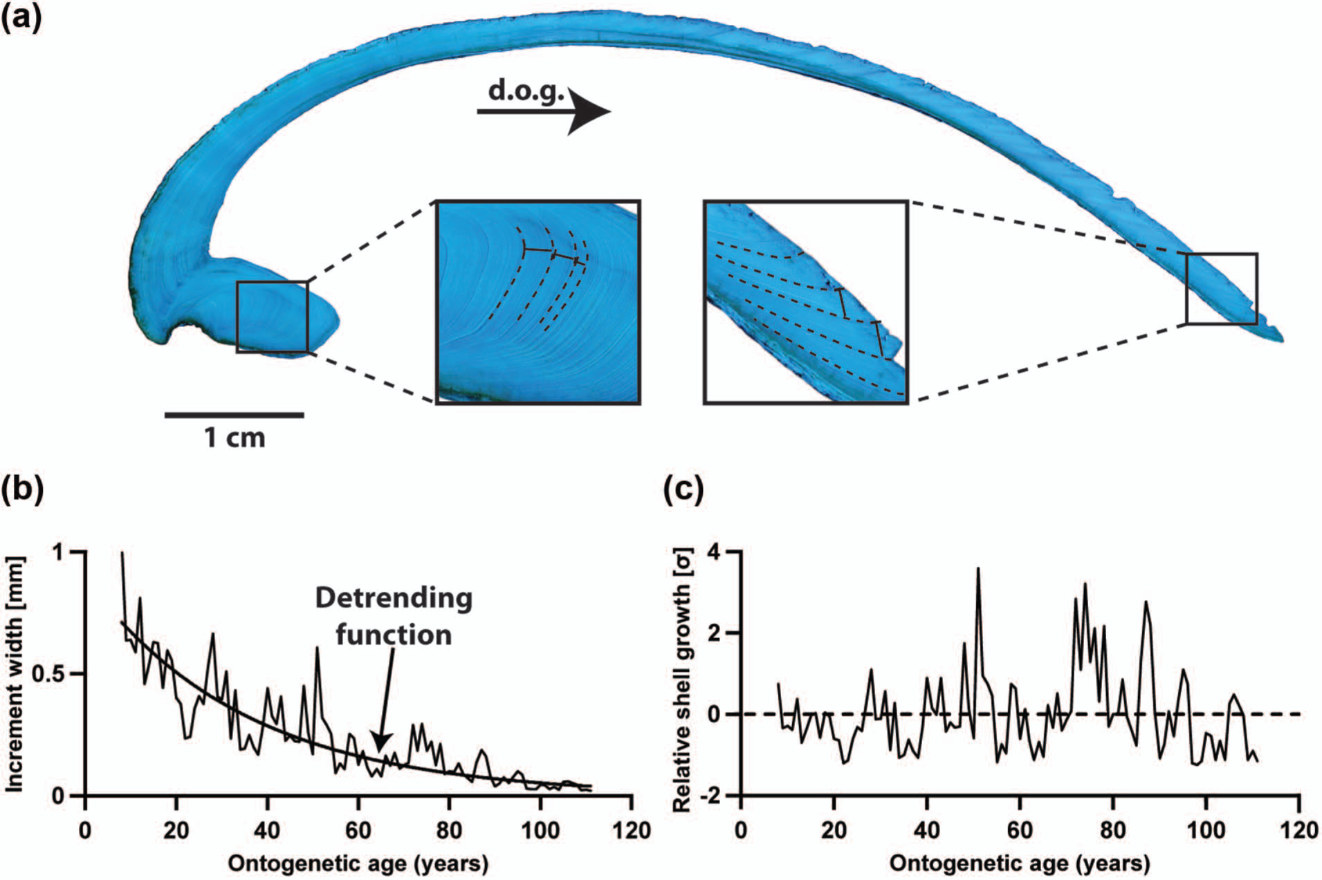
Sclerochronological analysis of Arctica islandica shells. (a) Cross-section immersed in Mutvei’s solution showing distinct annual growth lines and increments in the outer shell layer of the hinge portion (left) and the ventral margin (right). (b) Annual increment widths and the variance decrease through ontogeny. The trend toward narrower increments at later stages of life can be estimated with a growth function (‘detrending function’) and mathematically eliminated from the time-series. (c) After detrending and standardization, relative changes in shell growth can be studied.
Cross-dating and temporal alignment of the sclerochronologies
The precise calendar alignment of the increment width chronologies (Figure 3) was accomplished by three different cross-dating methods: (1) visual cross-dating applying wiggle-matching and identifying pointer years (Schweingruber et al., 1990), (2) the dendrochronology software COFECHA (Grissino-Mayer, 2001), and (3) the JAVA™-based Shell-Aligner© software (programmed by one of us, CL). The fundamental difference between the two computer-aided alignment methods is that COFECHA focuses almost exclusively on the year-to-year agreement (higher frequency domain; correlation coefficients), whereas Shell-Aligner cross-dates chronologies based on the best agreement in the high- and low-frequency realm after removal of ontogenetic age trends by means of regional curve standardization (RCS). Shell-Aligner uses algorithms developed for the comparison of amino-acid sequences in molecular cell biology (Needleman and Wunsch, 1970; Smith and Waterman, 1981). Whereas Shell-Aligner requires age-detrended growth increment width chronologies; COFECHA processes raw chronologies. COFECHA applies a high-pass filter (here, a flexible cubic spline adjusted with a rigidity of 32 years and 50% frequency response in accordance with Butler et al., 2013) to each of the raw increment width chronologies, computes normalized growth indices (ratios of measured divided by predicted growth values), removes the autocorrelation from the time-series, and provides suggestions for the temporal alignment of the data (least squares method) by indicating how the agreement could be increased by adding or deleting growth increments.
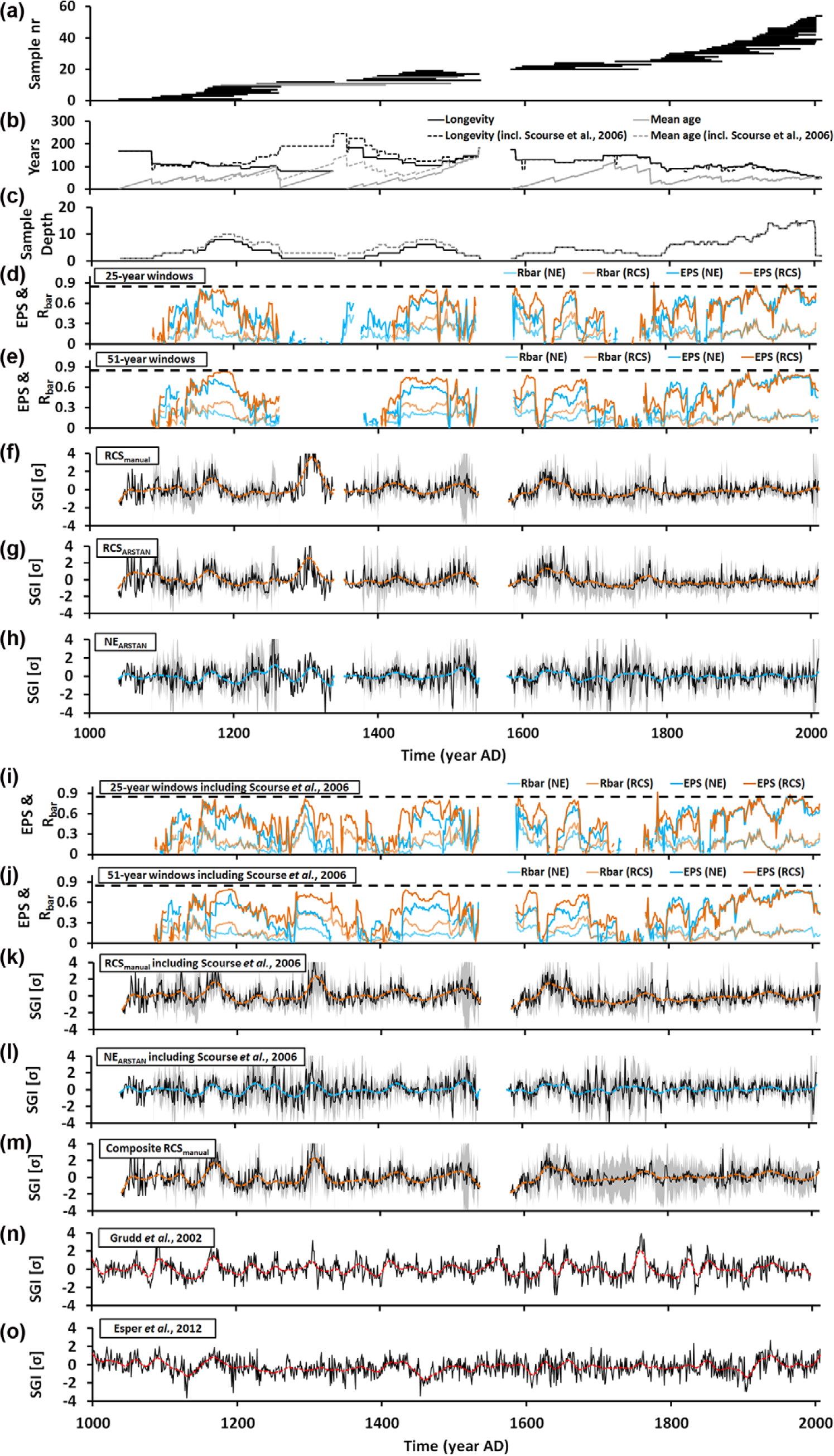
Multiregional Arctica islandica composite chronology from the North Sea and statistical measures. (a) Life spans of specimens. Each horizontal line corresponds to a single individual. Gray bars represent the three specimens used in the study by Scourse et al. (2006). (b) Longevity and mean age through time. (c) Sample depth = number of specimens per time interval. (d and e) Estimated population strength (EPS) and inter-series correlation coefficient (Rbar) in running 25- and 51-year windows. Dashed horizontal lines reflect the 0.85 threshold of Wigley et al. (1984). Standardized chronologies based on different detrending techniques: (f) RCSmanual, (g) RCSARSTAN, (h) NEARSTAN. Gray lines denote 95% confidence intervals. (i and j) Estimated population strength (EPS) of dataset, including the three time-series of Scourse et al. (2006) in 25- and 51-year windows. (k to m) Standardized chronologies based on different detrending techniques, including Scourse et al. (2006). (k) RCSmanual, (l) NEARSTAN, and (m) Composite chronology. (n and o) Scandinavian dendrochronologies (Esper et al., 2012; Grudd et al., 2002) shown for comparison with the bivalve sclerochronology. These tree-ring master chronologies were also used to cross-date floating chronologies and place 14CAMS dated fossil shells in a precise temporal context. Flexible cubic splines with a rigidity of 25 years f–h and k–o were computed to facilitate recognition of common low-frequency oscillations.
Based on these cross-dating techniques, annual increment width time-series of live-collected and fossil shells with overlapping life spans were precisely temporally aligned. Radiocarbon dates facilitated the cross-dating of fossil shells by placing them in a narrow temporal window of the past. Some fossil shells, however, did not overlap with modern shells or precisely chronologically aligned fossil shells. To assign absolute calendar dates to these shells, the chronologies were cross-dated with Scandinavian dendrochronologies (Esper et al., 2012; Grudd et al., 2002). This method has previously been used by Schöne and Fiebig (2009) and is based on the notion that bivalves from the North Sea and trees from northern Scandinavia share common signals. The presence of common environmental forcings on bivalves and trees has also been demonstrated by Black et al. (2009) and Black (2009) in the US NW Pacific.
Age-detrending and chronology construction
To isolate environmental signals, ontogenetic age trends (decreasing growth rates and decreasing year-to-year variance with increasing age) were removed from the shell chronologies by the following statistical methods (Figure 2): (1) Negative exponential (NEARSTAN) detrending and standardization using the dendrochronology software ARSTAN (Cook, 1986). In addition to low-pass filtering (trend estimation), ARSTAN pre-whitened the time-series (removal of lag-1 autocorrelation) and performed a variance stabilization (removal of high correlation between the local mean and variance, production of homoscedastic time-series; Cook and Peters, 1997). (2) Regional curve detrending and RCS, a less flexible age trend-elimination method (Briffa et al., 1992). For RCS, a single ontogenetic growth curve was computed for the hinge and ventral margin records of all studied specimens and then applied to eliminate ontogenetic age trends of individual shell chronologies. (1) A seventh-order polynomial fit was used to estimate the ontogenetic age trend of all studied specimens. Growth indices for each year were then computed by dividing measured by predicted growth. For the manually constructed RCS chronology (RCSmanual), GI values at each year were arithmetically averaged. For comparison with other chronologies, the resulting time-series was mathematically standardized by subtracting the mean and dividing by the standard deviation (SGI values). (2) In addition, ARSTAN was used for RCS, including pre-whitening of the shell growth data (RCSARSTAN). At each year, ARSTAN calculated a bi-weighted mean of the growth indices.
In order to strengthen the sample depth in older sections of the chronologies, three time-series of the Fladen Ground floating chronology by Scourse et al. (2006) were cross-dated and incorporated in further versions of the RCSmanual and the NEARSTAN series, respectively. Based on methodological differences, our RCSmanual detrending procedure was inapplicable to the Fladen Ground time-series. The latter were detrended by a relatively rigid, 75-year cubic smoothing spline that also preserves parts of the low-frequency domain.
To evaluate the agreement of shell growth dynamics among the different sampling areas, three local time-series were calculated (Norwegian Sea, RCSNORS; Doggerbank, RCSDogger; Eastern North Sea, RCSENS). Together with the standardized mean Fladen Ground record of Scourse et al. (2006), they were then used to compile an average composite chronology (composite RCSmanual), where each locality takes equal account. Given the low number of local time-series and the variable coverage of time (including temporal gaps) of each time-series, a ‘nested’ approach as demonstrated in Cunningham et al. (2013) and Wilson et al. (2010) or a procedure as in Reynolds et al. (2013) was not carried out.
The robustness of the chronologies was evaluated by the expressed population signal (EPS) value (Briffa and Jones, 1990; Wigley et al., 1984).
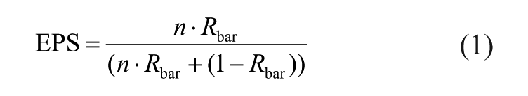
where Rbar is inter-series correlation between pairs of GI chronologies, and n is the number of specimens used to construct the stacked chronology. The EPS value quantifies how well the composite chronology resembles the infinitely replicated, perfect chronology (Briffa and Jones, 1990; Wigley et al., 1984). According to Wigley et al. (1984), EPS values greater than 0.85 indicate that the variance of a single SGI chronology sufficiently expresses the common variance of all SGI series. EPS values computed in running 25-year and 51-year windows were used to demonstrate how the agreement between the GI series changed through time.
Time-series analyses
To identify the temporal dynamics of the composite chronologies, continuous wavelet transforms (CWTs) were computed (parameter value = 6; Torrence and Compo, 1998; Figure 8) with MATLAB R2012b using the ion wavelet script, available online at http://ion.researchsystems.com/. In order to properly perform the spectral analyses, gaps in the shell chronology were filled with data of the Scandinavian tree-ring chronology (Esper et al., 2012; Grudd et al., 2002). A univariate red-noise autoregressive lag-1 (AR(1)) model was applied as a background spectrum to evaluate the 5% significance level, that is, the 95% confidence level of the CWT.
Spatial correlation maps (Figure 7) were computed between the different chronology versions (NEARSTAN, RCSmanual, RCSARSTAN, RCSNORS, RCSDogger, RCSENS) and meteorological data using the Koninklilijk Nederlands Meteorologisch Instituut (KMNI) explorer (Trouet and Van Oldenborgh, 2013; http://climexp.knmi.nl/; last checked: 15 January 2013). Instrumental datasets included (1) the NOAA Optimum Interpolation Sea Surface Temperature (OI-SST) Analysis dataset v. 2, hereafter referred to as Reynolds OI-SST (Reynolds, 1988; Reynolds and Smith, 1995; Smith and Reynolds, 1998); (2) SST of the Hadley Centre Sea Ice and SST dataset, HadISST (Rayner et al., 2003); (3) the European Reanalysis surface temperature dataset of the European Centre for Medium-Range Weather Forecasts, ERA-40 (S)ST (Uppala et al., 2005); (4) the ERA-40 sea surface pressure, ERA-40 SSP; and (5) zonal wind stress fields, ERA-40 zw. In addition, the NAO index (Hurrell, 1995) during February–September was compared with all chronology variants and the different seasonal averages of the environmental datasets listed above. Spatial regression analyses of the shell chronology variants (NEARSTAN, RCSmanual, RCSARSTAN) was only conducted for years containing at least four shells (=prior to 2002). Additionally to the spatial correlation attempts, simple regression analysis at monthly and seasonal resolution was performed between the A. islandica chronologies and the instrumental datasets (Figure 6).
Results
Cross-dated growth increment time-series of the studied specimens of A. islandica from different localities in the North Sea (Figure 1) cover the time interval of
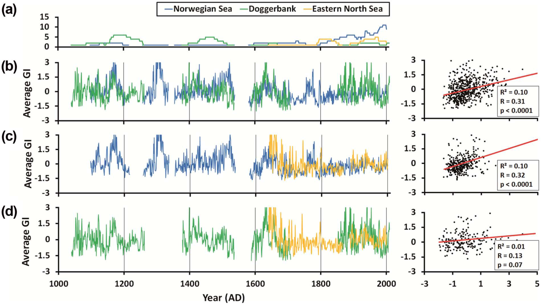
Comparison of growth signals between different localities of the present study. (a) Color-coded sample depths. Note, that the color-coding is maintained in the whole figure. (b–d) Regression analyses between the local RCSmanual GI time-series.
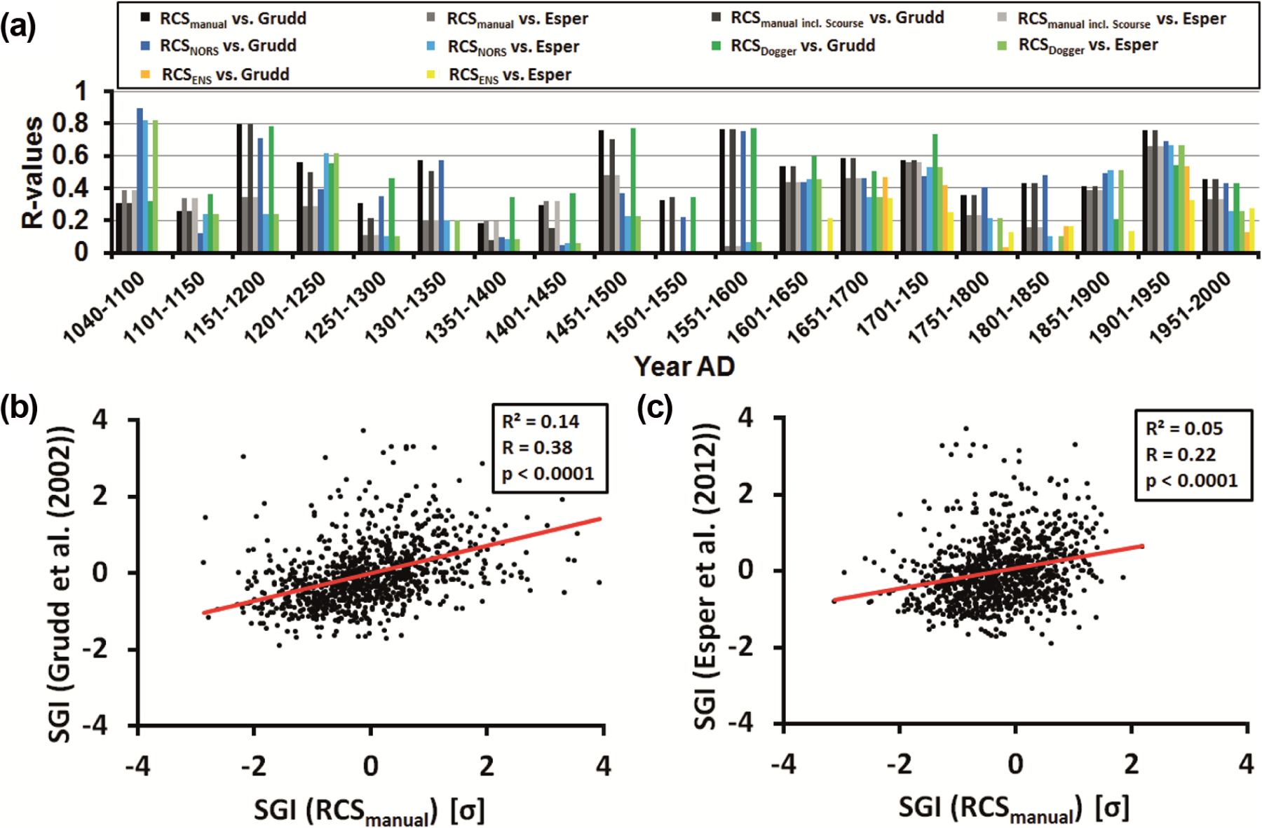
Regression analysis between the different shell chronology versions and the Scandinavian tree-ring reference chronologies. R values in 50-year segments (a) scatter plots between the whole RCSmanual chronology and both tree-ring time-series (b) Grudd et al. (2002) and (c) Esper et al. (2012).
During the 20th century, running EPS values exceeded the 0.85 threshold (Wigley et al., 1984). Prior to that time, EPS values remained below this critical threshold but were largely above 0.6 (Figure 3). EPS values closer to the critical threshold value defined by Wigley et al. (1984), that is, above 0.75 are normally accompanied by larger sample depths. Sharp signal declines were often associated with lower specimen numbers. Through cross-dating with the time-series by Scourse et al. (2006), it was possible to place the two oldest floating chronologies in an absolute temporal context and close the gap between the two time-series. However, because of the low sample depth, the EPS value still remained below 0.85. As expected by strongly fluctuating sample depths and the two major temporal gaps, average EPS values did not reach Wigley’s critical threshold value. The average EPS value of the NEARSTAN chronology (0.52, Rbar = 0.17, n = 5.31) returned a slightly lower value than the RCS time-series (0.56, Rbar = 0.19, n = 5.33). Versions that include the Scourse et al. (2006) time-series showed hardly any improvements concerning the population signal (RCSmanual: EPS = 0.57, Rbar = 0.19, n = 5.83; NEARSTAN: EPS = 0.53, Rbar = 0.16, n = 5.87). The regional chronologies exhibited lower EPS values (RCSNORS: EPS = 0.42, Rbar = 0.17, n = 3.66; RCSDogger: EPS = 0.57, Rbar = 0.29, n = 3.15; RCSENS: EPS = 0.43, Rbar = 0.19, n = 3.26). Maximum 25-year-running Rbar/EPS values ranged between 0.69/0.86 (NEARSTAN) and 0.81/0.91 (RCSmanual, RCSARSTAN; Figure 3).
Through the last millennium, the mean longevity of the studied specimens fluctuated between 49 and 184 years (Figure 3). During the ‘Little Ice Age’ (LIA), the average life span of A. islandica was 32 years longer than during the ‘Medieval Climate Anomaly’ and the Modern Warmth (Figure 3). Specifically, since the early 20th century, the average life span declined from 113 to 49 years (Figure 3). The oldest specimen of this study reached an ontogenetic age of 184 years. One shell of the Scourse et al. (2006) time-series was slightly older (227 years).
Fossil shells were not equally distributed through time, but exhibited four time intervals of high abundance, that is, c. 1170–1200, 1450–1475, 1640–1670, and after c. 1800 and four intervals of remarkably low abundance, that is, before c. 1085, 1260–1340, 1540–1580, and 1760–1790 (Figure 3).
Spectral analysis
Continuous wavelet transformation of five variants (NEARSTAN, RCSmanual, RCSARSTAN, RCSmanual with Scourse, Composite RCSmanual) of the chronology revealed distinct spectral power at frequencies corresponding to periods of 3–8, 12–16, 28–36, 50–80, and 120–240 years (Figure 8). The RCS chronologies were dominated by low-frequency oscillations (c. >28 years), whereas the higher frequency components were better preserved in the NEARSTAN time-series (Figure 8). All three RCS chronologies showed statistically significant (95% confidence interval) and temporally coherent signals in the 120- to 210-year band throughout the last millennium (Figure 8a, b, and d). Whereas these cycles are less developed in RCSARSTAN, they are pronounced in the chronologies that include the time-series of Scourse et al. (2006); these modes also occurred in the NEARSTAN time-series, but the 5% significance level was only reached between around 1400 and 1650, that is, the coldest interval of the LIA, including the Spörer and Maunder sunspot minima (Figure 8c). According to the NEARSTAN chronology, a transient shift occurred from higher frequency modes during the Medieval Warmth to low-frequency modes during the LIA, and back toward higher frequency oscillations during the Modern Warmth (Figure 8). In turn, these were lying mostly outside of the significance level.
Furthermore, we observed intermittently strong and highly significant (5% significance level) spectral density at periods of less than 80 years throughout the last millennium (Figure 8); 28–36 and 50–80 year bands dominated periods of sunspot maxima, for example, during the Medieval Warmth and between c. 1550 and 1670, whereas the strong and highly significant shorter wavelengths of 3–8 and 12–16 years were observed during the Spörer and Maunder Minima. In case of the Wolf Minimum, we observed higher frequencies directly before the period of reduced sunspot numbers (NEARSTAN). Yet, statistically significant higher frequency modes (3–8, 12–16 year cycles) were also found during warm phases (e.g. 1100–1200, 1740–1775, and since 1880).
Correlation with instrumental data
Annual shell growth was positively correlated with SST and zonal wind stress in the North Sea realm (Figure 6). Additionally, a positive correlation of shell growth and the NAO index was observed. Overall strongest correlations were found for shell growth and SST during April and November, and for SSP (sea surface pressure) and zonal wind stress between February and September. Spatial correlation coefficients were highest (>0.6) for RCSmanual and Reynolds OI-SST during 1982–2001 (Figures 6 and 7). Spatial regression analyses for longer time intervals (other surface temperature products and zonal wind stress) returned R values above 0.3–0.4 (Figure 7b–e). In case of HadISST, secondary linear detrending (=elimination of diverging linear trends) applied to the bivalve chronology and the instrumental time-series increased the agreement between the two chronologies. Spatial correlation patterns of the NAO were remarkably similar to that of shell growth and surface temperature, zonal wind stress, or sea surface pressure (Figure 7). According to the spatial regression approach, the similarities between the chronologies and environmental time-series were regionally specific. Furthermore, the local time-series (RCSNORS, RCSDogger, RCSENS) exhibited generally lower R values with the instrumental datasets than the multiregional chronology.
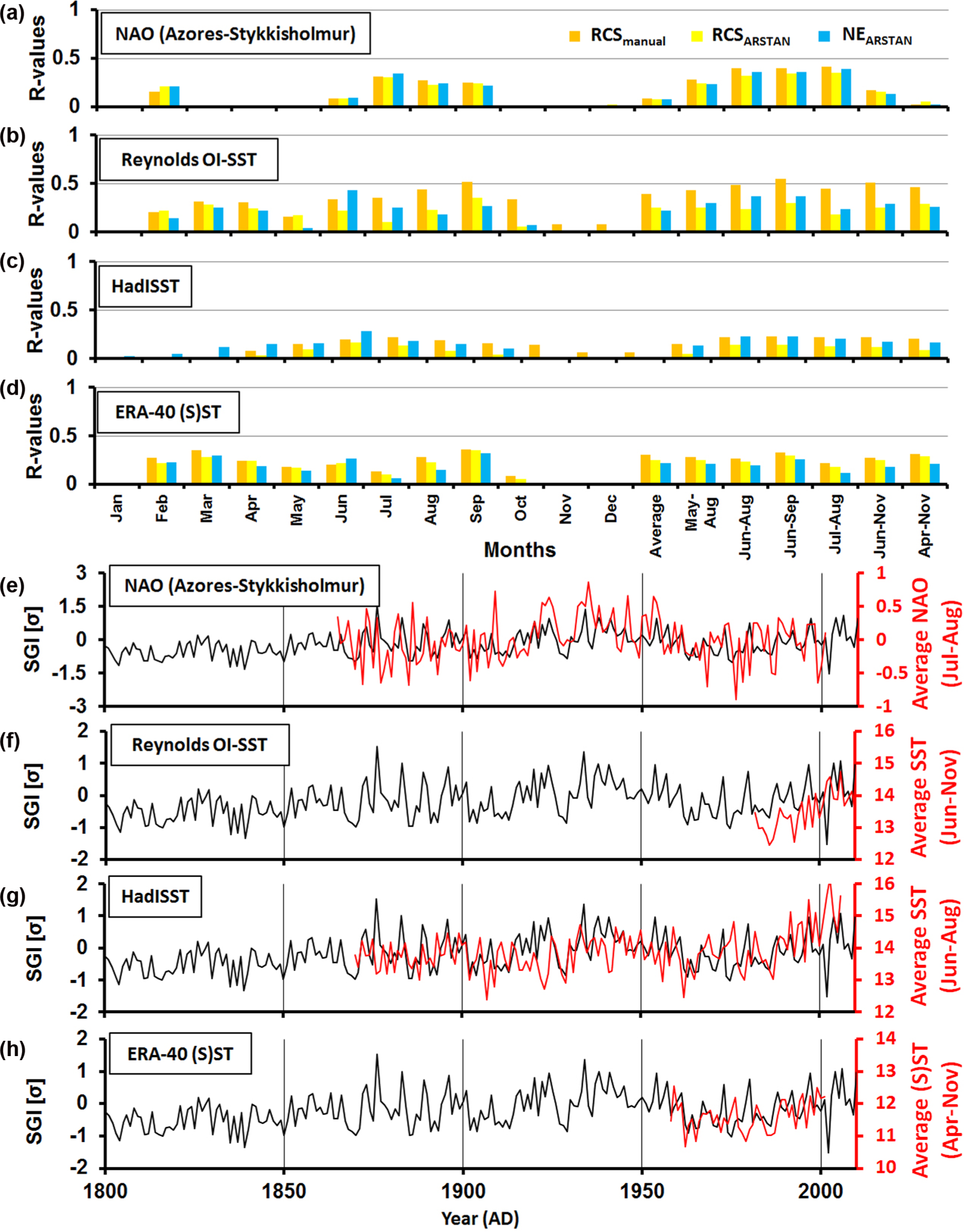
Calibration between the different versions of the North Sea bivalve sclerochronology with instrumental datasets. (a–d) Monthly and seasonally calculated R values with (a) North Atlantic Oscillation (NAO) Index (1900–2001), (b) Reynolds OI-SST (1982–2001), (c) HadISST (1900–2001), and (d) ERA-40 (S)ST (1958–2001). Except for NAO, instrumental datasets are spatially averaged over 50°N to 62°N and −2°E to −10°E. (e–h) Curve plots of RCSmanual with seasonally averaged instrumental records with the datasets of (a)–(d).

Spatial correlation maps. The three variants of the Arctica islandica chronologies (for sample depths >3 shells), the three local time-series of Norwegian Sea (NORS), Doggerbank (Dogger), and Eastern North Sea (ENS) as well as the North Atlantic Oscillation (NAO) index were compared with different (sea) surface temperature (SST) products, zonal wind stress and sea surface pressure (SSP). Increment-temperature comparisons were computed for the April–November average, that is, the main growing season of the bivalves. Regression intervals for sea surface pressure, zonal wind stress, and the NAO time-series are set from February to September. (a) Reynolds OI-SST: 1982–2001; (b) HadISST: 1900–2001; (c) a version using linear detrending of both the HadISST and the shell time-series; (d and e) ERA datasets (temperature, zonal wind stress, sea surface pressure): 1958–2001. Each comparison includes R values (left) and p values (right). Data points with probabilities above 10% in R value maps are drawn in pale colors.
Discussion
Since bivalve shell formation is governed by environmental conditions, growth curves of specimens with overlapping life spans can be cross-dated. Based on this method, it was possible to combine annual increment width chronologies of live-collected and fossil A. islandica specimens from different localities of the North Sea into chronologies covering nearly one millennium. Our time-series is the longest ever reported, absolutely dated bivalve sclerochronology from this region, offering a detailed insight into the climate history of the North Sea since 1040 and further contributing to the bivalve shell-based sclerochronological network (Butler et al., 2009a). Existing A. islandica chronologies from the North Sea covered the most recent 100–245 years (Butler et al., 2009a: 1870–1979; Epplé et al., 2006: 1840–2003; Schöne et al., 2003: 1757–2001; Witbaard et al., 1997: 1892–1991). Longer stacked records of A. islandica from the NE Atlantic came from the Skaggerak, Kattegat, and Øresund (Dunca et al., 2009: c. 200 years), the Irish Sea (Butler et al., 2009b: 489 years), and Iceland (Butler et al., 2013: 1363 years; Lohmann and Schöne, 2013: 508 years).
Spatial coherence of climate signals: multiregional chronology
An important difference to existing A. islandica chronologies (e.g. Butler et al., 2009a, 2009b; Witbaard et al., 1997) is the larger spatial coverage of the stacked record presented here. On the expense of synchronicity between individual time-series, our multiregional chronologies largely reflected supra-regional climate signals. The specimens that were used to construct the multiregional chronologies came from various different localities in the entire North Sea (Figure 1; Table 1) and were most likely exposed to very different local climate regimes. As a consequence, the agreement between increment width chronologies of contemporaneous specimens was lower than in many previous A. islandica studies. EPS values barely exceeded the 0.85 threshold even at times when six to eight specimens were available (Figure 3). For similar and lower sample depths, for example, Butler et al. (2013) reported EPS values greater than 0.95, indicating a large degree of running similarity. However, the shells used by Butler et al. (2009a, 2009b, 2012) were obtained from a much smaller region and belonged to the same population of bivalves. In fact, it is well known that the running similarity is largest among specimens of the same population, whereas the synchronicity decreases with increasing geographic distance between the populations (Marchitto et al., 2000). For example, in the northern North Sea (Fladen Ground), Butler et al. (2009a) found strongly coherent shell growth over distances of c. 80 km. In the same region, Witbaard et al. (1997) found common signals including variations at small regional scales as well. By sub-dividing our dataset into local chronologies, it became evident that the localities shared common environmental signals. Even though shell chronologies reached high internal correlations at the local scale, the multiregional chronologies exhibited only low EPS values indicating the preservation of local signals.
By combining time-series from many different localities, it was possible to capture over-regional climate signals. According to Dunca et al. (2009), low-frequency components of stacked A. islandica chronologies from the Skaggerak and Øresund (c. 300 km distance) were largely in phase. Likewise, spatial coherence of the chronologies presented here was also based on low-frequency signals which prevailed in the entire North Sea realm and especially at greater water depths exerted a strong control on A. islandica living at different localities in the North Sea and also influenced the growth of trees on land. However, this does not mean that the series were incongruent in the high-frequency domain (Figures 4 and 5).
Spatial coherence based on lower and higher frequencies can be used for cross-dating purposes (Fritts, 1976). This demonstrably works even across kingdom boundaries, that is, bivalve shells and trees (Black et al., 2009; Schöne and Fiebig, 2009). For example, Black et al. (2009) successfully cross-dated increment width chronologies of trees and geoduck shells, Panopea abrupta, in the NE Pacific to reconstruct SST. Schöne and Fiebig (2009) demonstrated the possibility to temporally align individual fossil shells of A. islandica through cross-dating with the Torneträsk dendrochronology (Esper et al., 2012; Grudd et al., 2002). This cross-dating concept was adopted in this study and used to assign precise calendar years to two 14CAMS dated floating chronologies (Figure 5).
Additionally, we tested two different procedures of constructing chronologies. Besides the conventional method of averaging all individual time-series, the composite chronology was generated with an arithmetic mean of the four local chronologies (RCSNORS, RCSDogger, RCSENS, Scourse et al., 2006). This approach has the advantage of weighing each locality equally. A major disadvantage is a significantly higher variance resulting from stronger influences of individual signals during time intervals of lower sample depths.
Since only two (‘F1’ and ‘F5’) of the Butler et al. (2009) time-series fit to the Witbaard et al. (1997) chronology (R1900–1979 = 0.1–0.11), it was difficult to compare the chronologies presented in this study with the shell growth dynamics at Fladen Ground. The Norwegian Sea sub-chronology compared best with the Fladen Ground chronologies and displayed the highest statistical agreement (R1900–1979 = 0.09–0.16). Furthermore, we observed a significant decrease in the correlation between the chronology of Witbaard et al. (1997) and our RCSNORS prior to 1975. A 1-year lag of the chronology by Witbaard et al. (1997) increased the correlation significantly (R1925–2000 = 0.19).
Climate oscillations
As reported in previous studies (Butler et al., 2012; Helama et al., 2007; Lohmann and Schöne, 2013; Schöne et al., 2003; Wanamaker et al., 2009), periodic changes in shell growth of A. islandica reflected well-known atmospheric and oceanic climate oscillations. For example, the high-frequency components in the 3- to 8-year and 12- to 16-year band seem to be most likely associated with the NAO and coupled ocean–atmosphere interactions in the subpolar North Atlantic (Deser and Blackmon, 1993; Dima and Lohmann, 2004; Park and Latif, 2005), respectively. It should be noted that high-frequency modes can be the product of random autoregressive memory effects (Wunsch, 1999). However, the spectral signal strength of the transitions exceeded the red-noise null hypothesis taking into account autoregressive processes.
The observed multi-decadal oscillations in shell growth (28–36, 50–80, 120–240 years) compare well with fluctuations in temperature and circulation patterns associated with AMOC and ultimately reflect temporal changes of the Atlantic water inflow into the North Sea (Witbaard et al., 1997, 2003). In order to interpret low-frequency signals, the so-called segment length curse has to be taken into consideration (Cook et al., 1995). The curse describes a fundamental problem of reduced low-frequency responses in time-series analysis that is coupled to detrending and standardization techniques. Here, this effect becomes evident by comparing the individually detrended NEArstan with the RCS chronologies. Whereas NEArstan is eliminating large portions of the low-frequencies, they are much better preserved in the RCS chronologies. Periodicities that exceed the average life span of specimens used in the composite chronology should be interpreted with caution.
Surprisingly, the strength and statistical significance of the different quasi-decadal and multi-decadal climate modes during the last millennium seem to be associated with the sunspot cycles as well as warm and cold periods (Figure 8). Atmospheric and coupled ocean–atmosphere signals (quasi-decadal components) were particularly pronounced during the sunspot minima (Figure 5). For example, the 3- to 8-year and 12- to 16-year periods were stronger at around 1500, that is, close to the beginning of the LIA (Lamb, 1965). Similar findings have been reported from other A. islandica composite chronologies and other climate proxy archives (Butler et al., 2013; Christiansen, 1998; Lohmann and Schöne, 2013). According to historical documents (Ogilvie and Jónsson, 2001), wind stress and the inter-annual climate variability were much higher during this climatic regime shift (Trouet et al., 2012).
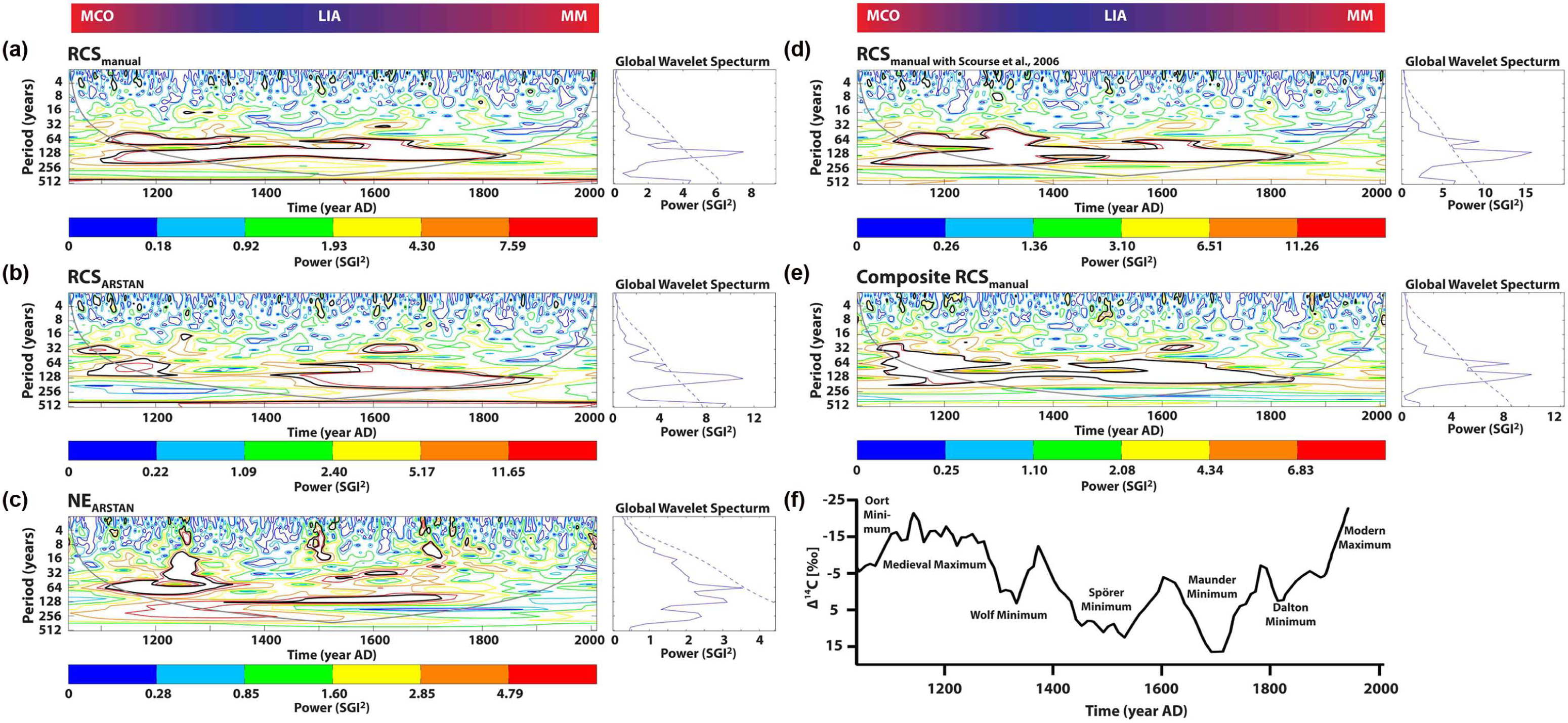
Wavelet transforms (wavenumber 6, Morlet wavelet) and global wavelet spectra of four variants of the Arctica islandica North Sea chronology as shown in Figure 3e–g, k and m. Temporal gaps in the chronology were filled with data from the Scandinavian dendrochronologies to enable calculation of continuous wavelet spectrum. (a) RCSmanual, (b) RCSARSTAN, (c) NEARSTAN, (d) RCSmanual filled with Scourse et al. (2006), and (e) Composite RCSmanual. Wavelet transforms provide information on the temporal evolution of signals. The power has been scaled by the global wavelet spectrum (at right). The contour levels are subdivided by the 90%, 80%, 65%, 50%, and 25% percentiles. Black contour is the 5% significance level, using a red-noise background spectrum. The cone of influence, where zero padding has reduced the variance, is illustrated by a gray line. Diagrams produced with MATLAB R2012b and the Ion wavelet script, online available at http://ion.researchsystems.com/). Note temporal changes of quasi-decadal and multi-decadal variability and their association with cold and warm phases and the sunspot number inversely reflected in the Δ14C record (f).
Warm intervals such as the Medieval Maximum, however, were dominated by signals in the range of 28–36 and 50–80 years, that is, the periodicity of AMOC. As a consequence, the northward heat transport became stronger and led to warmer conditions in the NE Atlantic realm (Lund et al., 2006; Wanamaker et al., 2012). Prolonged time intervals of stable climate conditions during the culmination phase of the LIA may be explained by the predominance of low-frequency variations (120–240 years) in oceanic heat transport.
In summary, stronger inter-annual to quasi-decadal variability was associated with a strong atmospheric forcing and outstanding sunspot minima. Occasionally, phases of increased climatic instability fell together with periods of high sunspots numbers. More stable climatic conditions (warm or cold), however, were observed in conjunction with a predominance of multi-decadal variability, maybe related to the AMOC. Whether a causal link exists between the sunspot number and the NAO as suggested by other authors (Van Loon et al., 2012) should be critically assessed in future studies and by including other annually resolved climate proxy records from the NE Atlantic realm.
Environmental controls on shell growth
According to spatial regression analyses (Figure 4), shells of A. islandica grew faster when surface waters were warmer and westerlies were stronger (positive NAO) between April and November. This correlation may be associated to the greater water depth in which the bivalves lived, where more constant conditions prevailed throughout the growing season. However, no direct link can have existed between the growth of bivalves that lived below the thermocline and environmental conditions prevailing at sea surface between spring and fall. Only when the thermocline disrupts in winter, warm surface waters are mixed downward and reach the sites where the bivalve lives (OSPAR Commission, 2000). It is more likely that faster growth of the bivalves is indirectly linked to surface water conditions. Higher productivity rates in warm surface waters were followed by higher levels of organic debris reaching the sea floor that nurtured the bivalves.
Conversely, increased westerlies associated with the NAO likely increased the speed of currents, which in turn can have resulted in increased amounts of re-suspended organic particles near the bottom of the sea, and hence increased food levels. A positive relationship between benthic productivity and decadal climate modes has also been identified in many previous studies (Kröncke et al., 2001; Witbaard et al., 1997). Decadal cycles of temperature and the availability and quality of food may also have influenced the reproductive success of A. islandica (recruitment cycles) and may serve as an explanation for the observed distribution of fossils through time (Figure 3). Apparently, maximum and minimum abundances of shells alternated periodically every c. 240 years (Figure 3). However, additional data are required to verify this hypothesis, for example, a statistically robust map showing the age distributions of A. islandica in various parts of the North Sea.
Temperature fluctuations may also explain the observed changes in average longevity of A. islandica during the last millennium. Although this species is well adapted to low temperature conditions and demonstrably grows during winter even at much higher latitudes (Schöne, 2008), colder water may result in reduced growth rates. Shells growing at lower rates during early ontogeny will likely reach the predation window and maturity at a later age than specimens growing quickly during youth. Therefore, slower growth rates can increase the life expectancy. Notably, the oldest ever reported specimens of A. islandica, for example, a 374-year-old ‘Methuselah’ from E Iceland (Schöne et al., 2005b) and a 507-year-old specimen from North Iceland (Butler et al., 2013) were born during the Spörer Minimum. Decreased average longevity during the 20th century, however, is more likely the result of overfishing in the North Sea (e.g. Coll et al., 2008).
Summary and conclusion
We presented the first multiregional A. islandica chronologies which cover nearly the entire 2nd millennium
In order to identify and quantify long-term climate trends through the last millennium, future studies should focus on the geochemical proxy record which is not subject to the ‘segment length curse’ (Cook et al., 1995). As demonstrated here, variations in shell growth can provide important information on decadal climate variability, but the reconstruction of longer term climatic oscillations and trends is limited by the length of the individual chronologies used to build the chronology.
Furthermore, a cross-calibration with other A. islandica composite chronologies from the northern North Atlantic (Butler et al., 2012; Lohmann and Schöne, 2013; Scourse et al., 2006; Wanamaker et al., 2008; Witbaard et al., 1997) as well as other high-resolution paleoclimate archives such as tree rings, speleothem records, varved sediments, and so on (Briffa et al., 1992; Esper et al., 2002; Fohlmeister et al., 2012; Grudd et al., 2002; Scholz et al., 2012; Sirocko et al., 2012; Vollweiler et al., 2006) can help to draw a more detailed picture of the climatic past of Europe. Such information is relevant to test, verify, and improve predictions of possible future climates in this region. The new EU-funded international collaboration Annually Resolved Archives of Marine Climate Change (ARAMACC) will certainly contribute to a better understanding of past European marine climate conditions.
Footnotes
Acknowledgements
Shells used in this study were kindly provided by Wolfgang Dreyer (University of Kiel, Germany), Ingrid Kröncke (Senckenberg am Meer, Wilhelmshaven, Germany), Ronald Janssen and Michael Tuerkay (Senckenberg Research Institute and Natural History Museum, Frankfurt/Main, Germany), Heye Rumohr (Geomar/Helmholtz Centre for Ocean Research, Kiel, Germany), and Annemiek Vink (Bundesanstalt für Geowissenschaften und Rohstoffe, Hannover, Germany). We are grateful to Paul Butler, James Scourse (School of Ocean Sciences, Bangor University), and Rob Witbaard (NIOZ, Royal Netherlands Institute for Sea Research) for providing bivalve sclerochronologies from Fladen Ground. We are greatly indebted to Michael Maus for his help during laboratory work. Furthermore, we want to express our thanks to Paul Butler and an anonymous reviewer for their helpful and constructive suggestions.
Funding
This study has been made possible by a PhD scholarship of the Earth System Research Center Geocycles (to HAH) and a grant by the German Research Foundation (DFG) (to BRS: SCHO793/10).