Holocene climate variability in Central Germany and a potential link to the polar North Atlantic: A replicated record from three coeval speleothems

Introduction

Speleothems offer a variety of advantages as climate archives and are increasingly used for paleoclimate studies (Henderson, 2006; Lauritzen and Lundberg, 1999). One of their advantages is that they occur in all continents except Antarctica (Ford and Williams, 2007), at a variety of latitudes and longitudes as well as altitudes (Spötl and Mangini, 2007). Using the ²³⁰Th/U disequilibrium method, speleothems can be dated with exceptional accuracy and precision up to an age of about half a million years (Richards and Dorale, 2003; Scholz and Hoffmann, 2008; Cheng et al., 2013). The most widely used paleoclimate proxies in speleothems are stable carbon and oxygen isotopes (e.g. Asrat et al., 2007; Baker et al., 2011; Mattey et al., 2008; Meyer et al., 2008; Spötl and Mangini, 2007; Spötl et al., 2008). Another group of widely used climate proxies are trace elements, which provide insights into the karst hydrology (Ayalon et al., 1999; Fairchild and McMillan, 2007; Finch et al., 2003; McMillan et al., 2005; Roberts et al., 1998, 1999; Treble et al., 2003; Van Beynen et al., 2008; Zhou et al., 2008a, 2008b), soil and vegetation characteristics (Hellstrom and McCulloch, 2000; Huang et al., 2001; Tooth and Fairchild, 2003) and may allow detection of anthropogenic impact in the catchment (Fairchild and Treble, 2009; Labuhn et al., 2015; Verheyden, 2004).

Here, we present stable isotope and trace element data from three late Glacial and Holocene stalagmites from the Herbstlabyrinth (HL) cave system, Central Germany, and use data from an extensive cave monitoring programme to support the interpretation in terms of past climate change. This study aims towards a better understanding of terrestrial climate variability in Central Europe during the late Glacial and the Holocene and in particular its relationship with the polar North Atlantic.

The late Glacial (i.e. the transition period between fully glacial and interglacial conditions, from 19 to 11.5 ka BP (thousands of years before 1950)) is characterized by large climate oscillations at both global and regional scales (Litt et al., 2003). Here, we focus on the Northern Hemisphere and in particular Central Europe. The δ¹⁸O record of the NGRIP ice core from central Greenland shows warmer climate conditions during the Bølling (14.64–14.03 ka BP) and a progressive cooling towards the end of the Allerød (14.03–12.85 ka BP). These time intervals were also characterized by several rapid oscillations from warmer to cooler conditions (Rasmussen et al., 2006). Between 14.45 and 13.35 ka BP, the vegetation in Central Europe changed from Arctic steppe tundra to open woodland with birch trees (Litt and Stebich, 1999). The onset of the Younger Dryas (12.85 ± 0.13 ka BP; Rasmussen et al., 2006) was characterized by rapid cooling (Litt et al., 2003) lasting until 11.65 ± 0.1 ka BP (Vinther et al., 2006). Litt et al. (2003) suggested a subdivision of the Younger Dryas into a first part which was relatively wet and cold, followed by a second part which was drier and warmer. During the Younger Dryas, the steppe tundra vegetation in Central Europe returned for more than 1 ka (Litt and Stebich, 1999).

The focus of this study is on the Holocene, which started at the end of the Younger Dryas at 11.65 ka BP (Vinther et al., 2006). This boundary is clearly visible in the NGRIP ice core by a rapid shift towards more positive δ¹⁸O values and similar shifts in deuterium excess and dust content, which occurred within ca. 3 years (Steffensen et al., 2008; Walker et al., 2009). This shift is interpreted as a change in atmospheric circulation, which was accompanied by a temperature change of 10 ± 4°C in Greenland (Walker et al., 2009). In addition, sea-surface temperatures in the source region of Arctic precipitation declined by ca. 2–4°C because of the reorganization of the Northern Hemispheric atmospheric circulation, shifting from the warmer mid-Atlantic during glacial times to colder high latitudes in the early-Holocene (Walker et al., 2009). During the last 8 ka, the δ¹⁸O values of the NGRIP ice core show relatively low variability, except for three prominent events: the 8.2 and 9.3 ka events and the Preboreal oscillation at 11.4 ka (Vinther et al., 2006). During the 8.2 ka event, January temperatures in Central Europe were lower than today, but the effect on the vegetation was not as pronounced as, for instance, in Scandinavia (Litt et al., 2009; Seppä et al., 2007). In contrast to the relatively stable conditions suggested by the δ¹⁸O values of the NGRIP ice core, various other studies suggest substantial climate variability during the Holocene. For instance, Bond et al. (1997, 2001) found cycles in the abundance of ice-rafted debris (IRD) in deep-sea sediments from the sub-polar North Atlantic which are occurring approximately every 1.5 ka. They interpreted these maxima in IRD as colder phases caused by a reorganization of ocean currents in the North Atlantic. Reconstructed July temperatures in Central Germany during the early-Holocene (around 9 ka BP) are comparable to present-day temperatures, whereas January temperatures were between 2 and 10°C colder than today (Litt et al., 2009). In addition, climate became progressively wetter during the Holocene (Litt et al., 2009). During the Holocene climate optimum (between about 8.5 and 5 ka BP), July temperatures in Central Europe were ca. 1°C warmer than today. The mid-Holocene climate optimum peaked at 6.7–6 ka BP (Davis et al., 2003; Litt et al., 2009). Subsequently, during the late-Holocene, summer temperatures declined again, whereas winter temperatures progressively increased (Davis et al., 2003). Litt et al. (2009) found high variability in January temperatures and precipitation in Central Germany around 5 ka BP. Prior to 6 ka BP, the pollen records show a natural succession of vegetation controlled by the development of soil, climate and competition of trees (Litt et al., 2009). Human impact is visible in Central Europe since ca. 7 ka BP and is mainly indicated by the decreasing abundance of forest indicators (arboreal pollen) and the increasing abundance of herb pollen suggesting more open habitats (Litt et al., 2009). This strong land use continues until today with regional differences depending on the fertility of soils (Litt et al., 2009).

Material and methods

Cave monitoring

Monthly aggregated samples of soil water, one under forest (SW1) and one under meadow vegetation (SW2, Supplemental Figure 1B, available online), were obtained at a depth of approximately 60 cm using soil suction probes. Soil air pCO₂ values were obtained at the same depth using a Vaisala MI-70 handheld meter and a Vaisala GMP222 Carbon Dioxide Probe coupled with a GM70 Aspiration Pump. The accuracy of the pCO₂ measurements is ±150 ppmv + 2% of the current reading. The values are corrected for air pressure (P) using the equation from Spötl et al. (2005):

C O 2 ( ppmv ) = C O 2 ( RAW ) * 1013 P

(1)

Air pressure was measured barometrically with a Sunartis BKT 381/B 381 device. The same instrumental set-up was used to measure the pCO₂ inside the cave. The cave monitoring programme is set up in a small chamber, close to the location where stalagmite HLK2 grew (Supplemental Figure 1C, available online). The drip rate was logged using a Stalagmate drip logger (www.driptych.com) at 1-h resolution. The logger records up to 5 drops per second. Additionally, the drip rate was measured manually every time the cave was visited. For this purpose, the number of drips amounting to 2 mL of drip water was counted and the corresponding time recorded. Three fast drip sites (Supplemental Figure 1C DR, available online) with an average drip rate of 0.4 drops per second were instantaneously sampled. In addition, a slow drip site with a water throughput of about 60 mL per month was also sampled (Mischel et al., 2015). Here, we only report the mean values of the three fast drip sites. During the monthly cave trips, water from a cave pool in the Kleine Kammer was also sampled (PW, Supplemental Figure 1C, available online).

All sampled waters were analysed for pH, electrical conductivity (EC), carbonate hardness, cations and anions as well as δ¹⁸O and δD. δ¹⁸O and δD values were measured using a ThermoFisher DELTA^plusXL mass spectrometer with a GasBench II and a ThermoFisher DELTA Advantage coupled to a TC/EA at the University of Innsbruck. These instruments were calibrated using VSMOW, GISP and SLAP. The long-term precision (1σ) of the δ¹⁸O and δD values is 0.08‰ and 1.0‰, respectively.

Cation concentrations of the drip water samples were determined at Heidelberg University using an Agilent ICP-OES 720. The internal 1σ-standard deviation is <1% for Ca, Mg, Ba and Sr. SPS SW2 was used as external standard and its long-term 1σ-reproducibility is 1.7% for Ca, 3.6% for Mg, 3.6% for Sr and 1.7% for Ba. PO₄³⁻ was measured spectrometrically (SPECORD 50 plus (Analytik Jena, Germany)).

Results

²³⁰Th/U-dating and age modelling

The results of ²³⁰Th/U-dating are presented in Supplemental Tables 1–3 (available online), and the age models constructed using StalAge are displayed in Figure 1. The ²³⁸U concentration of the stalagmites ranges from 0.02 to 0.3 µg g⁻¹. Sub-sample SM39 from stalagmite NG01 is not in stratigraphic order (Figure 1; Supplemental Table 1, available online). Since all other ages of the corresponding section are in stratigraphic order and indicate a constant growth rate, sub-sample SM39 is regarded as an outlier and discarded. The relatively large uncertainty at the beginning of the youngest growth phase of NG01 is a result of StalAge, which uses ensembles of three-point fits and, thus, attaches only little importance to individual ages in the border areas of individual growth phases (Scholz and Hoffmann, 2011). This is reflected by considerably enlarged age model uncertainties at the beginning and end of the growth sections, in particular in case of changes in growth rate (Scholz et al., 2012b). All other 22 ages determined of NG01 are in stratigraphic order (Figure 1). The recent growth of stalagmite NG01 is confirmed by extrapolation of the age model to the top of the stalagmite. The 18 ages obtained for stalagmite HLK2 are all in stratigraphic order within error (Supplemental Table 2, available online, Figure 1). The recent growth of this stalagmite, suggested by the wet surface when collected (Supplemental Figure 2B, available online), is not confirmed by the dating. The youngest age is 2.2 ka, and extrapolation of the age model suggests a top age of the stalagmite of 0.59 ± 0.28 ka. The lowest part of the stalagmite below the clay layer (indicated by the black arrow in Supplemental Figure 3B, available online) is older than 58 ka (Supplemental Table 2, available online) and not subject of this paper. The 12 sub-samples obtained on stalagmite TV1 are in stratigraphic order (Figure 1; Supplemental Table 3, available online).

OPEN IN VIEWER

Figure 1.

Depth–age models of stalagmites HLK2, TV1 and NG01 calculated using StalAge. Sub-sample SM39 not used for age modelling is marked in red.

The first growth period after the last Glacial started at 13.62 ± 0.13 ka BP (HLK2, Figure 1). Speleothem growth during the late Glacial is uncommon for caves in Central Germany (Niggemann et al., 2003). This early growth phase is constrained by five ages and lasted for about 550 years until 13 ka BP. The next sample, at a depth of 108 mm distance from top (dft), has an age of 11.99 ± 0.13 ka BP. Thus, HLK2 has a hiatus between 13 and 12 ka BP or at least a phase of very slow growth. However, since this phase corresponds to the Younger Dryas with lower temperatures and probably reduced vegetation, an interruption of speleothem growth is likely. Thus, we assume a hiatus during this phase (Figure 1). Stalagmites NG01 and TV1 started to grow at 11.13 ± 0.08 and 10.26 ± 0.08 ka BP, respectively. Stalagmite TV1 grew continuously until the present day. Stalagmite NG01 has two hiatuses, one between 8.81 ± 0.01 and 7.65 ± 0.06 ka BP and another between 4.96 ± 0.07 and 2.2 ± 0.04 ka BP (Figure 1; Supplemental Table 1, available online). Stalagmites HLK2 and TV1 (Supplemental Figure 4, available online) have slow growth rates between 5 and 35 µm a⁻¹. In contrast, the two older parts of stalagmite NG01 grew much faster (80–140 µm a⁻¹). The youngest growth phase again has a slower growth rate of approximately 40 µm a⁻¹ (Supplemental Figure 4, available online).

Stable isotope and trace element data

The δ¹³C values of the two host rock samples are between 1.6‰ and 2.9‰, the δ¹⁸O values range from −4.8‰ to −5.2‰. These results are in agreement with the values published by Richter et al. (2010), who found δ¹³C values between 1.8‰ and 2.7‰ and δ¹⁸O values from −1.0‰ to −5.3‰. These values are typical for Devonian limestone from the Rhenish Slate Mountains.

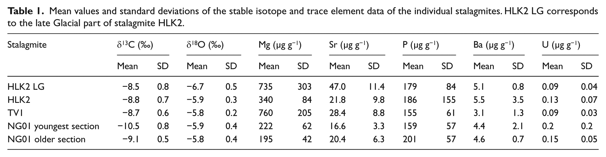
The stable isotope and trace element data of the three stalagmites are compiled in Figures 2–4; the values measured on the host rock are found in Supplemental Table 4 (available online). We present δ¹³C and δ¹⁸O values as well as the concentrations of Mg, Sr, P, Ba and U. The magnitude and variability of these proxies are comparable in all three stalagmites (Table 1). The long-term trend of all data sets was calculated by an interpolating spline with 5 degrees of freedom (Figures 2–4) using the smooth.spline function of R (R Core Team, 2016).

OPEN IN VIEWER

Figure 2.

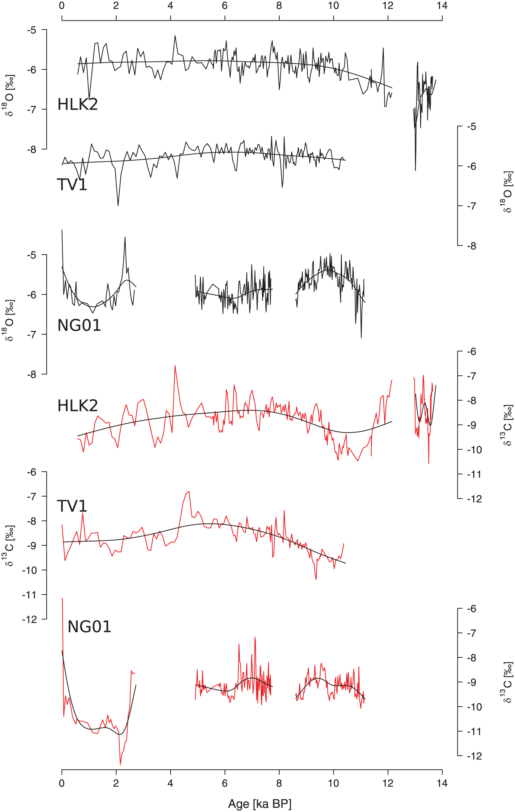
Temporal evolution of the δ¹⁸O and δ¹³C values of stalagmites HLK2, TV1 and NG01. The black lines are the long-term trends of the data.

OPEN IN VIEWER

Figure 3.

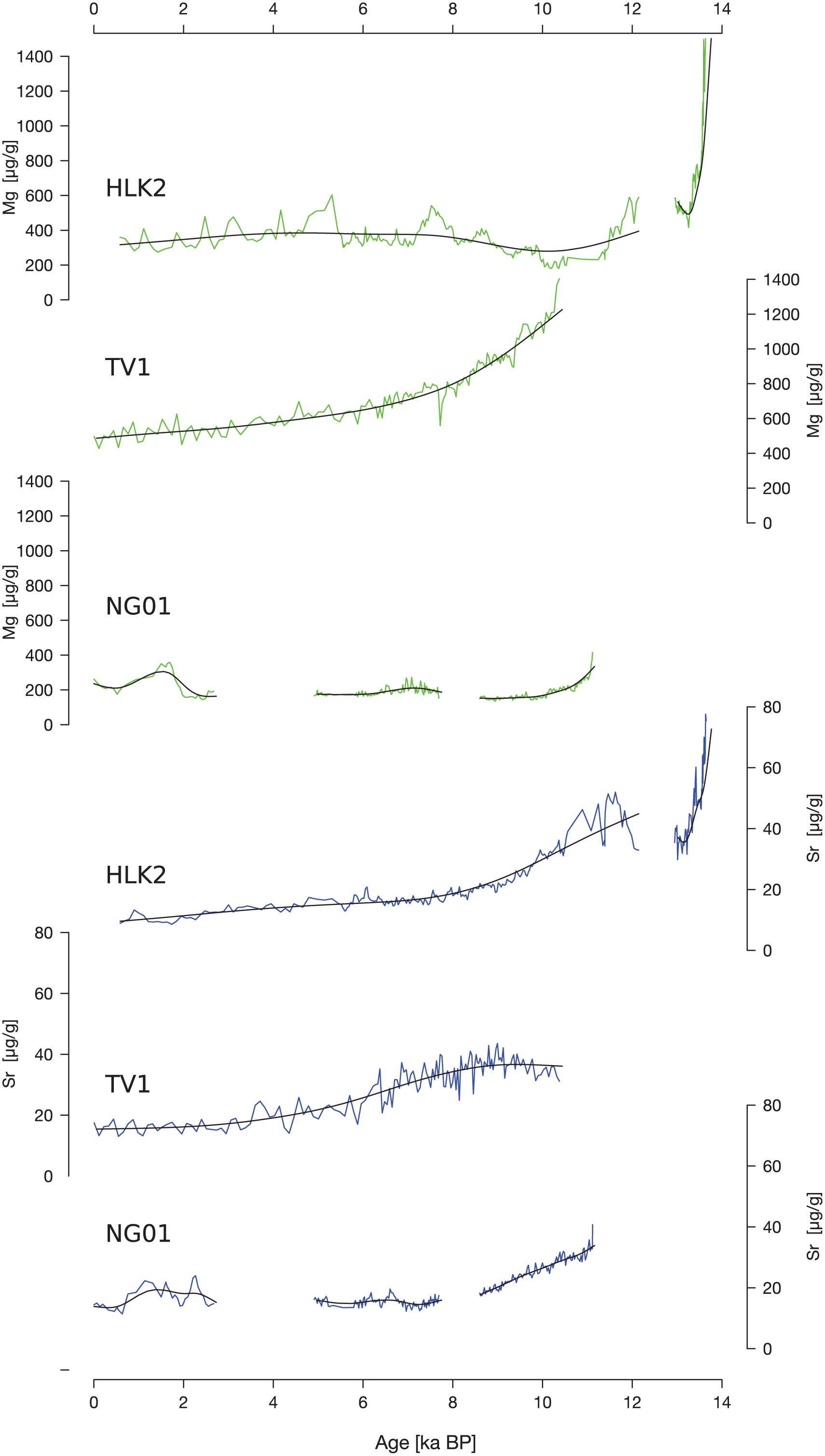
Temporal evolution of the Mg and Sr concentrations of HLK2, TV1 and NG01. The black lines are the long-term trends of the data.

OPEN IN VIEWER

Figure 4.

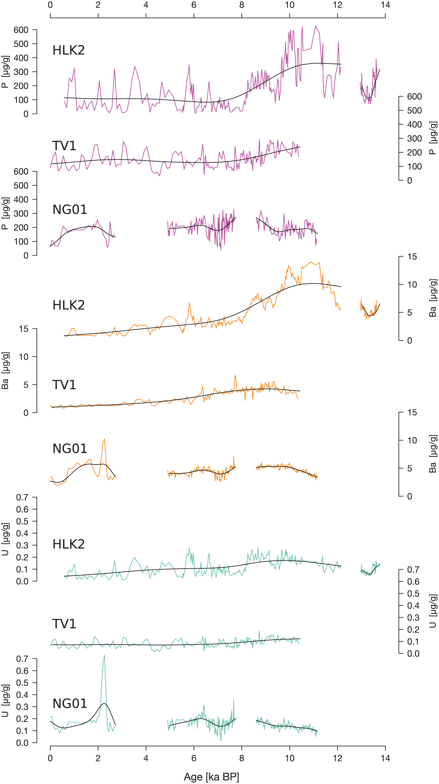
Temporal evolution of the P, Ba and U concentrations of HLK2, TV1 and NG01. The black lines are the long-term trends of the data.

OPEN IN VIEWER

Table 1.

Mean values and standard deviations of the stable isotope and trace element data of the individual stalagmites. HLK2 LG corresponds to the late Glacial part of stalagmite HLK2.

Stalagmite	δ13C (‰)		δ18O (‰)		Mg (µg g−1)		Sr (µg g−1)		P (µg g−1)		Ba (µg g−1)		U (µg g−1)
	Mean	SD	Mean	SD	Mean	SD	Mean	SD	Mean	SD	Mean	SD	Mean	SD
HLK2 LG	−8.5	0.8	−6.7	0.5	735	303	47.0	11.4	179	84	5.1	0.8	0.09	0.04
HLK2	−8.8	0.7	−5.9	0.3	340	84	21.8	9.8	186	155	5.5	3.5	0.13	0.07
TV1	−8.7	0.6	−5.8	0.2	760	205	28.4	8.8	155	61	3.1	1.3	0.09	0.03
NG01 youngest section	−10.5	0.8	−5.9	0.4	222	62	16.6	3.3	159	57	4.4	2.1	0.2	0.2
NG01 older section	−9.1	0.5	−5.8	0.4	195	42	20.4	6.3	201	57	4.6	0.7	0.15	0.05

The early growth phase of stalagmite HLK2 is generally characterized by more negative δ¹⁸O values (Figure 2, Table 1) and a decreasing trend after the onset of growth during the Bølling/Allerød. During the Younger Dryas, stalagmite HLK2 stopped growing. With the onset of the Holocene, the δ¹⁸O values increase in all three stalagmites. In HLK2 and TV1, the δ¹⁸O values record a distinct depression around 8.2 ka, whereas this phase is represented by a hiatus in stalagmite NG01 (Figure 2). The remaining part of the Holocene is characterized by variable δ¹⁸O values without a strong trend in both HLK2 and TV1. NG01 shows a trend in the δ¹⁸O values in the youngest part, with larger values at the beginning and end of the growth phase. The δ¹³C values of stalagmites HLK2 and TV1 are comparable and indicate a similar long-term trend. Both stalagmites exhibit relatively low δ¹³C values at the beginning of the Holocene followed by a trend towards more positive values starting around 10 ka BP. The most positive values are observed between 8 and 4 ka BP. Subsequently, the δ¹³C values decrease towards the present day. The evolution of the δ¹³C values of stalagmite NG01 is different, as a mid-Holocene maximum recorded by the other stalagmites is not present (Figure 2). Furthermore, stalagmite NG01 has a distinct minimum in δ¹³C around 2 ka BP (Figure 2) and rapidly increasing δ¹³C values towards the present day. Both patterns are not visible in the other records. Nevertheless, the magnitude of the δ¹³C values of NG01 is generally comparable with that of the other stalagmites (Table 1).

Visible in the late Glacial part of HLK2 is a strong negative trend in both Mg and Sr with high initial values followed by rapid decrease (Figure 3). Whereas the Mg content of TV1 decreases during the Holocene, the Holocene Mg records of HLK2 and NG01 values decrease during the early-Holocene and are relatively stable afterwards (Figure 3). Interestingly, the mean Mg content of the Holocene part of stalagmite HLK2 is about twice as high as that of NG01 despite of the general similarity of the long-term signals (Table 1). The Sr content decreases during the Holocene in all three stalagmites and, thus, has a similar long-term pattern (Figure 3).

In P, Ba and U, the same long-term pattern is visible in the late Glacial part of stalagmite HLK2 with decreasing concentrations at the beginning and increasing concentrations towards the end. The evolution of these three elements is also comparable in the Holocene sections of the three stalagmites. Phosphorus and Barium in HLK2 have higher concentrations at the beginning of the Holocene, followed by a progressive decrease. Between 10 ka BP and today, TV1 has a similar long-term pattern as HLK2. The Uranium content slightly decreases in the long-term trend in all stalagmites. As for the other proxies, the long-term evolution of the P, Ba and U content of NG01 is slightly different, in particular in the youngest section of the stalagmite. The mean values of the three elements agree well between the three stalagmites (Table 1).

Discussion

Speleothem proxy signals (both stable isotope and trace element signals) may be influenced by a variety of processes (Fairchild et al., 2006; Fairchild and Treble, 2009; Lachniet, 2009; McDermott, 2004). Thus, their interpretation in terms of past climate variability, in particular, during phases of relatively stable climate such as the Holocene, may not be straightforward. A multi-proxy approach to coeval stalagmites from the same cave provides the advantage that common robust features of the records, driven by a general process (e.g. a change in precipitation above the cave), may be extracted. This may enable to disentangle the various processes influencing the proxy signals from each other as well as the climate signals from the intrinsic noise of the specific cave system. In order to identify common features of the different proxy signals, we performed correlation and principal component analysis (PCA) of the data sets of the individual stalagmites. For improved comparability, NG01 was divided into two parts separated by the ca. 2.2-ka-long hiatus at 4.9 ± 0.07 ka BP (Figures 1–4). The older part has substantially higher growth rates than the younger part (Supplemental Figure 4, available online). Similarly, stalagmite HLK2 is separated by the hiatus into the late Glacial and the Holocene part.

To avoid artificial correlations because of long-term trends, we detrended all records using an interpolating spline with 5 degrees of freedom (Figures 2–4), which was subtracted from the data set. The long-term trends can be considered as reflecting orbital-to-millennial-scale information, whereas the detrended records reflect centennial-to-decadal-scale variability. Both signals may, in principle, contain paleoclimate information.

In the following, we first discuss the δ¹⁸O records of our stalagmites and compare them with other paleoclimate archives. Subsequently, the δ¹³C and trace elements data are discussed in greater detail based on the results of the statistical analyses.

δ¹⁸O values

The detrended δ¹⁸O values of the speleothem records are not significantly correlated with the other proxies (Supplemental Figure 5, available online). The exception are the δ¹³C values, which exhibit weak-to-moderate positive correlations with the δ¹⁸O values in the Holocene growth phases, except the youngest part of NG01. In addition, the δ¹⁸O values of the older section of stalagmite NG01 have a weak positive correlation with the Mg concentration. This suggests that the δ¹⁸O values are influenced by different processes than the other proxy signals weakening potential correlations. It is well known that speleothem δ¹⁸O signals are influenced by a variety of different processes occurring in the atmosphere (affecting the δ¹⁸O value of precipitation), in the soil and the karst aquifer as well as inside the cave (Dreybrodt and Scholz, 2011; Lachniet, 2009). Our recent study of drip water δ¹⁸O values based on cave monitoring and meteorological data (Mischel et al., 2015) showed that the δ¹⁸O values of the drip water at the HL are influenced by a complex interplay of different processes. Mischel et al. (2015) examined the influence of the NAO on drip water δ¹⁸O values at the HL and concluded that the reconstruction of the NAO from speleothems at the HL is challenging if not even impossible. The most important factors biasing the present-day speleothem δ¹⁸O signal are the even distribution of precipitation at the HL throughout the year and the slow growth rate of speleothems, precluding the reconstruction of seasonal climate signals. This suggests that the interpretation of speleothem δ¹⁸O signals at the HL during the climatically stable period of the Holocene is difficult as has also been shown for other cave systems (Scholz et al., 2012a). This is further supported by the reconstruction of precipitation from Litt et al. (2009); they reconstructed relatively stable rainfall amounts during the last 5 ka for Central Europe.

Although the interpretation of the δ¹⁸O values is challenging, comparison with other records may provide information on supra-regional climate patterns. Figure 5 shows a comparison of the three speleothem δ¹⁸O records with the δ¹⁸O values of the NGRIP ice core, the lake Ammersee ostracod δ¹⁸O record (Von Grafenstein et al., 1999) and a stacked speleothem δ¹⁸O record from nearby Bunker Cave (Fohlmeister et al., 2012). The Allerød is recorded in stalagmite HLK2, and its isotope pattern compares well with that of NGRIP and Ammersee.

OPEN IN VIEWER

Figure 5.

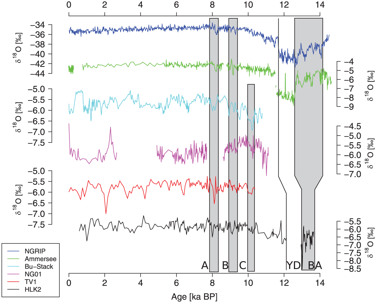
Comparison of the δ¹⁸O values of speleothems NG01 (magenta), TV1 (red) and HLK2 (black) with the δ¹⁸O records from NGRIP (blue, Vinther et al., 2006), Ammersee (green, Von Grafenstein et al., 1999) and Bunker Cave (cyan, Fohlmeister et al., 2012). Light grey boxes indicate the Bølling/Allerød (BA) as well as the 10.0 (C), 9.1 (B) and 8.2 (A) ka events (Boch et al., 2009). Also indicated is the Younger Dryas (YD) to Holocene transition (solid line). The dark grey boxes indicate phases with similar evolution of the δ¹⁸O values at the HL and Bunker Cave.

At the beginning of the Younger Dryas, the speleothem δ¹⁸O values decrease abruptly. Subsequently, stalagmite growth ceased, which is probably related to the rapid cooling and drying at the beginning of the Younger Dryas (Björck et al., 1996; Litt et al., 2009). After the Younger Dryas, speleothem growth at the HL recommenced. The generally increasing δ¹⁸O values between the Younger Dryas and ca. 10 ka BP as visible in the NGRIP and Bunker Cave record are clearly visible in both the HLK2 and the NG01 δ¹⁸O records (Figure 5). This suggests that on the millennial scale, speleothem δ¹⁸O values at the HL reflect large-scale climate variability in the North Atlantic area. In stalagmites HLK2 and TV1, the 8.2 ka event is expressed as a pronounced negative δ¹⁸O excursion (Figure 5). The timing of the event is in agreement with both stalagmites and also agrees with the negative excursion recorded in the Ammersee, NGRIP and Bunker Cave records. The 8.2 ka event is not preserved in Stalagmite NG01, there is a hiatus. In stalagmite HLK2, a negative excursion at 9.1 ± 0.2 ka BP might coincide with the 9.1 ka climate anomaly in the Alps as reported by Boch et al. (2009). This event is also recorded in other paleoclimate archives and other regions, for instance, in a stalagmite from Dongge Cave in China (Dykoski et al., 2005) and in the Ammersee record (Figure 5). However, the other speleothem δ¹⁸O records (NG01 and TV1) and the Bunker Cave record do not show this event as a pronounced excursion. In addition, all speleothem records from the HL show a pronounced trough between 10.3 and 10.0 ka which is also clearly visible in the Bunker Cave record. This event probably corresponds to the supra-regional cooling event discussed by Boch et al. (2009). Considering the proximity of Bunker Cave and the HL (Supplemental Figure 1, available online), the δ¹⁸O records at the two cave sites are expected to be similar. However, except for the prominent cooling phases discussed above, the records do not show striking similarities. For instance, the large positive peak in the Bunker Cave record during the ‘Little Ice Age’ is not visible in the speleothems from the HL. This may be related to the slow growth of NG01 and TV1 during this period. The differences between the δ¹⁸O signals at the HL and Bunker Cave may either result from the dating uncertainties or effects occurring in the local karst aquifers.

δ¹³C values and trace elements

The growth rates of stalagmites HLK2 and TV1 are relatively low and more or less constant over the entire Holocene (~10 µm a⁻¹; Supplemental Figure 4, available online). The growth rate of NG01 is much higher (~80 µm a⁻¹), even in the youngest part (~40 µm a⁻¹; Supplemental Figure 4, available online). The most likely explanation for this difference is that the drip rate of the stalactite that fed stalagmite NG01 was much higher and/or that the supersaturation with respect to calcite of the drip water feeding this stalagmite was higher. Since the gallery was destroyed by quarrying before our study was conducted, this cannot be confirmed by monitoring. Nevertheless, it seems to be a common pattern for all stalagmites that growth rates are higher during the early growth phases and lower and rather constant during the last 4–6 ka (Supplemental Figure 4, available online). Since both drip rate and supersaturation may have a substantial effect on speleothem stable isotope values (Mühlinghaus et al., 2009; Riechelmann et al., 2013; Scholz et al., 2009) and trace element concentrations (for instance, because of their influence on prior calcite precipitation (PCP), Fairchild and Treble, 2009), this may have important consequences for the proxy signals recorded in the stalagmites. Thus, differences between NG01 and the other stalagmites need to be considered in the interpretation of the proxy records.

Supplemental Figure 5 (available online) contains the correlation matrices of the detrended data set of all stalagmites. Phosphorus, Barium and Uranium are positively correlated throughout the Holocene, except for the youngest part of NG01. Phosphorus originates from the host rock (dissolution of apatite), serves as a plant nutrient and is recycled biogeochemically (Fairchild and Treble, 2009). A more productive vegetation cover leads to more leaf litter, which will then be leached and flushed into the cave leading to a higher P concentration of the cave drip water (Borsato et al., 2007; Huang et al., 2001). Figure 6 shows that the seasonal pattern of phosphate concentration in the drip water indicates flushing of phosphate into the cave during autumn and winter. Figure 6 also shows the drip rate, which peaks during winter months at the HL (Mischel et al., 2015). Since the retention time of the drip water is about 10 months (Mischel et al., 2015), transmission of the trace element signals into the cave should lag the peaks in drip rate by ca. 1 year and consequently not affect the seasonal pattern. Thus, the monitoring data confirm our hypothesis. More productive vegetation also leads to increasing soil pCO₂ because of the higher degree of soil microbial activity and root respiration. This is also clearly visible in the monitoring data from the HL, which reveals a pronounced seasonal cycle in soil pCO₂ (Figure 6). The related change in the acidity of soil CO₂ may influence the Ba content of the drip water (Hellstrom and McCulloch, 2000), which should consequently lead to higher values during spring and summer months. However, the Ba content of the drip water peaks in winter months and is anti-correlated with soil pCO₂ (Figure 6). This suggests that Ba, similar to P, is flushed into the cave during autumn and winter when drip rates are higher. As U is positively correlated to P and Ba, the U content also seems to be related to vegetation. The U content of the drip water can also be influenced by the change from more oxidizing to more reducing conditions in the soil regime with U being more mobile in oxidized environments (Hellstrom and McCulloch, 2000). We interpret P, Ba and U as proxies for vegetation productivity above the cave, with increasing concentrations of all elements reflecting a stronger intensity of nutrient cycling. This is a function of the availability of leaf litter, root respiration and biological activity, which correlate with a more productive vegetation.

OPEN IN VIEWER

Figure 6.

Multiannual changes in Mg, Sr and Ba and PO₄ concentrations of the drip water at the Herbstlabyrinth cave system. Also shown are drip rate, δ¹³C values of the DIC of the soil and drip water as well as soil gas pCO₂.

Figure 4 displays the long-term trend of P, Ba and U in the three stalagmites. These elements have a similar trend, in particular in stalagmites HLK2 and TV1, with higher values during the early-Holocene, which progressively decrease towards the recent past. This may reflect a gradual depletion of the source of these elements, for instance, a loess cover, as has been suggested for other sites (Fohlmeister et al., 2012). Stalagmite NG01 has a different long-term pattern, probably because of the different growth rates.

The Magnesium content of speleothems has been interpreted as a proxy of effective precipitation (Fairchild and Treble, 2009; McMillan et al., 2005). A longer residence time in the karst aquifer, because of a reduction in precipitation and recharge, leads to a prolonged contact of the water with the host rock. Even if the water is saturated with respect to calcite, it may still leach Mg from the host rock because of the lower solubility of dolomite. This, in turn, leads to elevated Mg concentrations in the drip water (Fairchild and Treble, 2009; Roberts et al., 1998). Higher Mg concentrations in the drip water thus reflect less recharge and vice versa. In most of our stalagmite records, Mg is negatively correlated with P, Ba and U and positively correlated with δ¹³C (Supplemental Figure 5, available online). This indicates less Mg and consequently increased recharge during times of more productive vegetation, probably reflecting wetter conditions. We note that more productive vegetation may also lead to increased transpiration and, thus, a reduction in recharge (Mischel et al., 2015). If evapotranspiration exceeds summer rainfall, this leads to a deficit in soil moisture, which might be reflected by decreasing drip rates in the cave (Mischel et al., 2015). If the amount of rainfall remains constant, more productive vegetation would result in a higher Mg content of the drip water because of a longer residence time of the groundwater. Since we observe the opposite in the speleothems from the HL, this effect either seems to be negligible or is compensated by additional summer rainfall. Mischel et al. (2015) explained that summer rainfall currently contributes 40% to the annual precipitation.

Interestingly, Strontium has a significant positive correlation with Ba in all records but no correlation with P and U (Supplemental Figure 5, available online). In the late Glacial part of HLK2, Sr is positively correlated with Ba and negatively correlated with P and U (Supplemental Figure 5, available online). This suggests that the variability of these trace elements was influenced by different processes during this period. The positive correlation with Sr suggests that Ba may also be influenced by PCP. This process should generally result in elevated Mg, Sr and Ba concentrations (Stoll et al., 2012) as well as increasing δ¹³C values (Johnson et al., 2006). The positive correlation between Sr, Ba and Mg in the drip water (Figure 6) thus supports PCP and/or a higher degree of CO₂ degassing during times of low drip rates (Johnson et al., 2006). Drip water δ¹³C values have a different trend than drip water Mg, Sr and Ba contents (Figure 6) indicating a different process dominating the δ¹³C signal (discussed in detail below). In the stalagmite records, Sr and Ba are positively correlated, whereas Mg is negatively correlated with Ba and negatively or even not correlated with Sr (Supplemental Figure 5, available online). This suggests that PCP either did not occur during the Holocene or was masked by another process, which has a more pronounced effect on the trace element signals.

If PCP is dominant, a positive correlation between Mg and Sr would be expected because of the suppressed incorporation of Mg and Sr into calcite in comparison with Ca. This effect is enhanced during times of reduced rainfall since more air-filled voids in the aquifer increase the potential for PCP (Fairchild and Treble, 2009; Huang et al., 2001). Another process resulting in a positive correlation between Mg and Sr is selective leaching of minerals in the soil (e.g. loess; Huang et al., 2001). A positive correlation between Mg and Sr is only observed in the late Glacial part of stalagmite HLK2 (Supplemental Figure 5, available online), suggesting that neither of these processes (PCP and selective leaching) were dominant during the Holocene. We observe a slight decrease in the Mg/Ca and Sr/Ca ratio of the drip water during the winter for the fast drip site (Supplemental Figure 6, available online). However, the total variability of the Mg/Ca and Sr/Ca ratios is relatively low. For the slow drip site, the Mg/Ca and Sr/Ca ratios decrease during winter months (Supplemental Figure 6, available online). This indicates the influence of PCP at the slow drip site during summer. This contrasts with winter; when the aquifer is filled with water, the effect of PCP is diminishing. However, since Sr and Mg are not correlated in the Holocene stalagmite records, PCP was either of minor important or masked by other processes.

All stalagmite records show a long-term decrease in Sr content during the Holocene (Figure 3). A potential explanation for this trend is that both Mg and Sr originate from a thin loess cover that was deposited during the last Glacial, which has then been progressively leached during the Holocene. Fohlmeister et al. (2012) observed a similar long-term trend in Mg content during the Holocene in a speleothem record from nearby Bunker Cave and proposed an identical mechanism.

Speleothem δ¹³C values are negatively correlated with P, Ba and U, which is visible in the Holocene records of HLK2 and TV1 as well as the older part of NG01 (Supplemental Figure 5, available online). The δ¹³C values of the host rock are between 1.6‰ and 2.9‰, and the vegetation above the cave consists mainly of C3-plants. The corresponding δ¹³C values of the soil air should therefore be between −26‰ and −20‰. The δ¹³C values of the stalagmites range from −10.4‰ to −6.6‰. These values, thus, reflect a partially open system, where the δ¹³C values are influenced by both the soil CO₂ respired by the C3-plants and the host rock (McDermott, 2004). Modelling studies suggest a relationship between the δ¹³C values of the drip water and soil pCO₂, with more negative δ¹³C values corresponding to higher soil pCO₂ (Fohlmeister et al., 2011). This relationship is also clearly reflected in the seasonal cycle of the δ¹³C values of the soil water and soil pCO₂ at HL (Figure 6). The most negative δ¹³C values of the soil water are measured shortly after the highest values in soil pCO₂. In contrast, no clear relationship between soil pCO₂ and the δ¹³C values of the cave drip water is observed (Figure 6). This is probably related to mixing and retention of the recharge water inside the aquifer. Since the monitored drip sites exhibit continuous dripping throughout the year, they are probably fed by a large reservoir in the epikarst. This is also confirmed by the study of Mischel et al. (2015), who estimated a mixing time in the epikarst of about 12 months and a transmission time (i.e. the time the water needs to travel through the host rock) of about 10 months. The effect of mixing leads to a smoothing of the seasonal proxy signals in the drip water. The long-term trend shows increasing δ¹³C values from the early- to the mid-Holocene and decreasing values until the present day (Figure 2). Processes occurring on shorter time scales, such as changes in cave ventilation and/or disequilibrium stable isotope fractionation (Deininger et al., 2012; Scholz et al., 2009), are unlikely to affect the δ¹³C signals on millennial time scales. A mature soil containing large amounts of soil organic matter is characterized by higher soil pCO₂ values and consequently low soil δ¹³C values (Fohlmeister et al., 2011). A potential explanation for the observed millennial-scale changes in the δ¹³C values during the Holocene, thus, is a progressive change in soil thickness and composition above the cave. An alternative explanation is a change in the type of vegetation above the cave. However, since the observed changes in δ¹³C values are small (in the range of 2–3‰, Figure 2), major changes in the type of vegetation (e.g. from C3- to C4-plants) are unlikely.

PCA

In order to gain further insight into the behaviour of the speleothem proxy data and the corresponding processes, we performed PCA using the trace element and stable isotope records of the three stalagmites. PCA was performed using R and the package psych (Revelle, 2015). Prior to PCA, the data were detrended using an interpolating spline with 5 degrees of freedom (Figures 2–4) and normalized using standard methods. PCA analyses multivariate data sets and calculates the contribution of the individual signals to the total variance of the data set. The number of variables is reduced to a lower number of new variables (i.e. the principal components (PCs)), preserving as much of the variation of the original variables as possible. The PCs can be used to identify common structures in the data and are often more easily interpreted than the initial multivariate data set (Jolliffe, 2002). A scree plot of the eigenvalues versus the PCs allows visual determination of how many meaningful PCs are required to explain the data (by detection of the kink, Supplemental Figure 7 (available online), Jolliffe, 2002). In all PCAs, the kink occurs at PC 2 (Supplemental Figure 7, available online), suggesting that at least two PCs are required to explain the data set. Whereas PC 1 explains ca. 50% of the variance, PC 2 only explains ca. 20% (Figure 7; Supplemental Table 5, available online). Thus, PC 2 is only briefly discussed in the following.

OPEN IN VIEWER

Figure 7.

Results of PCA of the individual growth phases of stalagmites HLK2, TV1 and NG01. Black and red numbers express the loading on PC 1 and PC 2, respectively.

For the late Glacial part of stalagmite HLK2, PC 1 explains 53% of the variance. P and U have strong, negative loadings on PC 1, while Mg, Sr, Ba and δ¹³C have a positive loading (Figure 7; Supplemental Table 5, available online). PC 2 explains 20% of the variance, and Sr and Ba have positive loadings, whereas δ¹³C and Mg have a negative loading. The strong covariation of Mg, Sr, Ba and δ¹³C in PC 1 indicates that PCP may have played a dominant role during the late Glacial (Figure 7; Supplemental Table 5, available online). However, since other trace elements also contribute to PC 1, this explanation is not straightforward. The negative loadings of P and U indicate that PC 1 – at least to some extent – also reflects vegetation processes. PC 1 and PC 2 explain 72% of the total variance of the late Glacial part of stalagmite HLK2 (Supplemental Table 5, available online).

PC 1 of the Holocene section of stalagmite HLK2 explains 51% of the variance and is composed of P, U, Ba, Sr, δ¹³C and Mg, with strong positive loadings of P, Ba and U, a strong negative loading of δ¹³C, a medium positive loading of Sr and a medium negative loading of Mg (Figure 7; Supplemental Table 5, available online). As discussed above, the most likely process to explain this pattern is that P, Ba, U and δ¹³C reflect changes in vegetation density. The PCA of TV1 has a similar pattern. PC 1 explains 46% of the variance and is also composed of P, Ba, U, Sr and δ¹³C and Mg (Figure 7; Supplemental Table 5, available online). As in stalagmite HLK2, Sr has a positive loading on PC 1, whereas Mg has a negative loading (Figure 7; Supplemental Table 5, available online). The positive relationship between Mg and δ¹³C and the inverse relationship between Mg and P, Ba and U indicate more humid conditions during times of more dense vegetation and enhanced nutrient recycling. This also confirms that PCP, which should result in a positive relationship between Mg and Sr, did not play a dominant role for the HL speleothems during the Holocene. Stalagmite NG01 is composed of two major growth phases with different growth rates (Figure 1; Supplemental Figure 4, available online). Growth rate can have a substantial effect on proxy signals. For instance, the incorporation of trace elements into calcite can be different at higher growth rates (Fairchild and Treble, 2009; McMillan et al., 2005). Furthermore, at higher recharge (and consequently higher speleothem growth rates), more particles and colloids are commonly flushed into the cave and incorporated into the speleothem (Fairchild and Treble, 2009). Therefore, the two growth phases are analysed separately. PC 1 of the oldest growth phase of NG01 explains 51% of the variance and is composed of P, Ba and U, which have a strong positive loading, and Mg and δ¹³C, which have strong negative loadings (Figure 7; Supplemental Table 5, available online). As discussed above, this probably reflects changes in the productivity of vegetation, in agreement with the other stalagmites. The negative relationship with Mg again suggests that periods of a more productive vegetation coincided with more humid conditions.

The youngest growth phase of NG01 shows the most contrasting PCs (Figure 7; Supplemental Table 5, available online). PC 1 is composed of Ba, U and Sr, having strong positive loadings, and P and δ¹³C have weak negative loadings. The positive relationship of U, Sr and Ba may again indicate a relationship with vegetation productivity, but the negative relationship with P is different from all other growth phases (Supplemental Figures 4, 5 and 7, available online). PC 2 is composed of δ¹³C and Mg, having positive loadings, which may reflect PCP and drip rate–dependent isotope fractionation effects controlled by the recharge of the karst aquifer. The negative loading of P on PC 2 (Figure 7; Supplemental Table 5, available online) is also different from the behaviour of this element during all other growth phases. In general, the patterns of this part of the stalagmite seem to be more complex than those of the other growth phases.

PC 2 generally explains a lower percentage of the complete variance of the proxy records (20–24%, Figure 7; Supplemental Table 5, available online). Therefore, the processes reflected by PC 2 are less clear, and the results are only briefly summarized here. PC 2 of the Holocene section of stalagmite HLK2 explains 20% of the variance and is composed of Sr, P and U (Figure 7; Supplemental Table 5, available online). Whereas Sr has a strong negative loading, U and P have intermediate negative loadings. PC 2 of stalagmite TV1 explains 24% of the variance and is composed of Sr, Ba and P (Figure 7; Supplemental Table 5, available online). PC 2 of the oldest growth phase of NG01 explains 23% of the variance and is mainly composed of Sr, which has a strong positive loading. Mg and U have negative loadings.

In summary, PCA shows a common pattern for all stalagmites, whereby PC 1 explains about 50% of the total variance in Holocene growth phases. PC 1 is composed of P, Ba and U, which have positive loadings, and δ¹³C and Mg, which have negative loadings. Therefore, PC 1 is interpreted as a proxy for the productivity of vegetation and precipitation, with higher values of Ba, U and P and lower values of Mg and δ¹³C reflecting a more productive vegetation and higher rainfall. A potential explanation for this pattern is that wetter climate fosters more productive vegetation. Conversely, during drier phases with decreasing vegetation (indicated by low P, U and Ba as well as high Mg and δ¹³C values), the soil and aquifer above the cave contain less water allowing increased ventilation. As a consequence, the karst dissolution regime may change towards a more open system. This has been demonstrated for speleothem records on annual, decadal and even centennial time scales (Fohlmeister et al., 2011; Griffiths et al., 2012; Noronha et al., 2014). A more open system results in lower δ¹³C values of the drip water and speleothem calcite (Fohlmeister et al., 2011). The δ¹³C records from the HL show the opposite behaviour with higher δ¹³C values during phases with elevated Mg and lower P, Ba and U concentrations. A potential explanation could be lower soil gas δ¹³C values because of water stress on plants (Cerling, 1984). Another explanation is a change in carbonate chemistry. Lower soil pCO₂ because of reduced vegetation density results in higher pH values of the drip water saturated with respect to calcite and higher δ¹³C values of the drip water and, thus, in the speleothem (Fohlmeister et al., 2011). As periods of lower vegetation density coincide with drier conditions at the HL, the elevated δ¹³C values could also result from isotope fractionation under disequilibrium conditions or enhanced PCP (Deininger et al., 2012; Johnson et al., 2006). The latter would also be consistent with the positive correlation between δ¹³C and Mg.

Comparison of the different stalagmite records

In the previous section, we studied each stalagmite separately, which revealed consistent patterns in all samples, such as the positive relationship between P, Ba and U, which is interpreted as reflecting past changes in vegetation productivity. These elements are often negatively correlated with δ¹³C, further corroborating this relationship. However, the PCA also revealed differences in the behaviour of the individual proxies between different stalagmites and even different growth phases of the same stalagmite. These characteristics may be related to differences in the hydrological pathways feeding the individual drip sites, which is also evident from the very different growth rate of stalagmite NG01. Replicated proxy records are, thus, very useful to separate site-specific from climate-driven processes.

In order to identify common features of the individual records and to eliminate site-specific effects, we compare the PCs rather than individual proxy signals. Figure 8 shows a comparison of the first PC of all three speleothems. Since the sign of the columns of the rotation matrix obtained by the PCA is arbitrary, the meaning (explanation) of the PC has to be established separately for each element (see description of the R package prcomp, R Core Team, 2016). Comparison of PC 1 with the individual trace element and stable isotope records allows deriving an interpretation of PC 1 (Supplemental Figure 8, available online). PC 1 of HLK2 has positive peaks when the proxies for vegetation productivity (P, Ba and U) have low values, and the δ¹³C values and the Mg concentration are elevated (Supplemental Figure 8, available online). This suggests that higher values of PC 1 correspond to a lower productivity of vegetation. In contrast, PC 1 of TV1 has higher values for elevated P, Ba and U values and lower δ¹³C values (Supplemental Figure 8, available online). Thus, higher values of PC 1 of this stalagmite correspond to more productive vegetation. PC 1 of the older part of NG01 has the same pattern as TV1 (Supplemental Figure 8, available online).

OPEN IN VIEWER

Figure 8.

Comparison of the PC 1 of stalagmites HLK2 (black), TV1 (red) and NG01 (magenta) with the HSG record (blue, Bond et al., 1997, 2001). Since the interpretation of PC 1 of stalagmite HLK2 is opposite than that of TV1 and NG01 (see main text), the y-axis is inverted for this record. The y-axis of the HSG record is also inverted. ²³⁰Th/U-ages with corresponding errors are plotted on top of the individual stalagmite records. Individual Bond events are labelled. The event 4/5 is suggested to be an additional Bond event. Vertical lines indicate phases of lower vegetation productivity potentially corresponding to Bond events. Dashed lines indicate events, which cannot be clearly assigned to a specific Bond event but may possibly be related to Bond events considering the relatively large dating uncertainties.

Comparison with supra-regional climate variability

Figure 8 shows a comparison of PC 1 of the three stalagmite records with the record of hematite-stained grains (HSGs) from North Atlantic deep-water sediments (Bond et al., 2001). Periods of high HSG values correspond to higher amounts of drift ice and, thus, reflect cool phases in the North Atlantic (Bond et al., 2001). Based on this relationship, Bond et al. (1997, 2001) distinguished nine cooling events (the ‘Bond events’, labelled 0–8 in Figure 8) occurring approximately every 1.5 ka, which were shown to be closely related to Central European winter temperatures (Mangini et al., 2007). Interestingly, most HSG maxima have corresponding peaks in PC 1 of the three HL stalagmite records (Figure 8). This becomes even clearer if the dating uncertainties of all records are taken into account. High percentages of HSG correspond to low values in PC 1 of stalagmite TV1 and NG01 and high values in PC 1 of stalagmite HLK2 (inversely plotted in Figure 8), suggesting a less productive vegetation and drier climate at the cave site during Bond events.

Bond events 8–6 are clearly visible in the stalagmite records from HL (Figure 8). Bond et al. (2001) marked two peaks of high percentages of HSG as Bond event 5. Since the duration of this event is ca. 1000 years long (Figure 8), we propose to divide this event up into two separate events on the basis of our stalagmites (labelled 5a and 5b, Figure 8). Both events have corresponding peaks in PC 1 of stalagmite TV1. PC 1 of stalagmite HLK2 has a small negative peak during event 5b and a clear negative peak during event 5a. Stalagmite NG01 has a hiatus in this phase. Both stalagmites (HLK2 and TV1) suggest a relatively low vegetation productivity interrupted by short-term events. Interestingly, the 8.2 ka event occurs during this phase, but both stalagmite records do not suggest a major drop in the productivity of the vegetation. Between Bond events 5 and 4, the HSG record also has a small peak (labelled 4/5 in Figure 8), which has not been labelled as a Bond event. This event has a clear expression in our speleothem records. On this basis, we assign this phase as an additional short-term Bond event. Bond events 4 and 3 are clearly visible in all speleothem records (Figure 8). Event 4 seems to be interrupted by a productive vegetation phase in speleothem HLK2. Bond event 2 seems to have lasted longer than recorded by the HSG record. The relatively short Bond event 1 is visible in PC 1 of all speleothems. However, the age models of the stalagmites are associated with relatively large uncertainty in the youngest section (Figure 1). Bond event 0 is reflected in all speleothems (Figure 8). As for event 1, the correspondence in stalagmite HLK2 is uncertain, which may be related to the large uncertainties of the age model (Figure 1).

In summary, each Bond event has a corresponding peak in PC 1 of at least one HL stalagmite. Some events are reflected in all stalagmite records. Since PC 1 is interpreted as reflecting the productivity of vegetation and precipitation, this suggests an influence of North Atlantic climate variability on vegetation density in Central Germany. In case of cooler climate, the vegetation is less productive and vice versa. However, based on the variability of PC 1 (Figure 8), the HL stalagmites record more phases of reduced vegetation density than suggested by the Bond et al. (2001) record. For instance, all stalagmite records suggest a phase of less productive vegetation between 7.0 and 6.2 ka BP (event 4/5 in Figure 8), which has only a relatively small counterpart in the HSG record. During Bond events 2 and 5, at least two peaks in PC 1 are visible in all stalagmite records (Figure 8). This suggests that these events may be divided up into two parts. In total, we identified 11 phases of less productive vegetation in our stalagmite records (Figure 8), which in most cases have equivalents in the Bond events.

Conclusion

Multi-proxy records from three speleothems from the HL cave system reflect several phases of less productive vegetation during the Holocene, which are manifested in lower P, Ba and U concentrations and more positive δ¹³C values. The negative correlation of Mg with P, Ba and U and the positive correlation with δ¹³C also indicate less recharge during phases of less productive vegetation, probably because of drier conditions. These patterns are clearly reflected in both the correlation analyses and the PCA.

The majority of the observed phases of reduced vegetation productivity and drier climate coincide with cooler periods in the polar North Atlantic as reflected by a higher abundance of HSG (Bond et al., 1997, 2001). This suggests a close relationship between terrestrial climate in Central Europe and the polar North Atlantic, even if the timing and duration are slightly different for some of the events. We also identified additional phases of less productive vegetation, which do not have a counterpart in the HSG record, indicating a different (maybe regional) trigger for these phases.

During the Younger Dryas, no stalagmite growth is observed at the HL, which is probably related to lower temperatures and reduced precipitation during this interval. The speleothem δ¹⁸O records are in general agreement with the NGRIP δ¹⁸O record on the millennial time scale, which is, for instance, reflected by increasing δ¹⁸O values between the Younger Dryas and ca. 10 ka BP. This suggests that speleothem δ¹⁸O values at the HL reflect large-scale climate variability of the North Atlantic region. This is also confirmed by the 8.2 ka event, which is clearly visible as a pronounced negative excursion in the speleothem δ¹⁸O values. However, in all other proxies, the 8.2 ka event is not well reflected.

In summary, this multi-proxy speleothem study suggests a close relationship between climatic conditions in the polar North Atlantic and Central Europe during the Holocene and highlights the potential of speleothem trace element records for high-resolution paleoclimate reconstruction.