Sediment geochronology for bar-built estuaries subject to flood deposition and erosion: A robust multiproxy approach across an estuarine zone

Abstract

This paper presents a contiguous late Anthropocene ²¹⁰Pb sediment geochronology and a late Anthropocene flood/fire event geochronology for an estuary subject to flood deposition and erosion. The procedure used multiple proxies to identify and evaluate flood facies overlying regions of erosion. Reconstructions of the original baseline sediments were undertaken for the major ²¹⁰Pb geochronological methods. Only the lower estuary core site, which was deficient in inventory of excess ²¹⁰Pb of baseline sediments, over the expected atmospheric supply for, was chosen to calculate the total amount of erosion. Erosion, as both cumulative mass and thickness, was then proportioned across flood events, relative to the size of the Rp index flood signal. The Rp index is the product of a simple stepwise thermogravimetric procedure. The flood geochronology was constructed by correlating the relative magnitudes of pivotal floods from an existing 100-year rainfall/river flow model and correlations in peak sediment char content outside of the flood facies with contemporary fire records. Overall, it was determined that ²¹⁰Pb sediment isotope tomography gave the closest convergence with flood and fire events over those of the constant rate of supply and constant initial concentration methods. The agreement signified that around 40% of the original baseline accretion (25 cm) had been eroded by floods over the last 83 years and that there was possibly considerably more erosion at the upper site, which led to the loss of two flood facies.

Keywords

bar-built estuary flood deposits Little Swanport River Estuary sediment erosion sediment isotope tomography

Introduction

Healthy seagrass meadows, which often inhabit shallow bar-built lagoons and estuaries (Short et al., 2007), are key in the sustainable economic and social well-being of the users of waterways (Barbier et al., 2011; De Groot et al., 2012). There is a growing realisation, however, that successful management of such large bodies of water requires the measurement and understanding of emergent long-term responses (Habeeb et al., 2007; Wiens and Milne, 1989). Such a long-term commitment from society is not often realised (Strayer et al., 1986). In response, researchers have started to produce their own long-term ecosystem time series. This is done by reconstructing ecosystem variability down the sediment column of the central heterotrophic deep spot from the convergence of multiple ecosystem proxies (Inkpen and Wilson, 2009). The deep spot acts as a sump, which integrates landscape scale ecosystem change across the shallower surrounding macrophyte bed with a corresponding long-term change (Carpenter and Leavitt, 1991; Engstrom and Wright, 1984; McGowan et al., 2005).

Success in interpreting the dynamics of any reconstruction depends on accurate and precise sediment column geochronologies. More often than not, the geochronology is based on the radioactive decay profiles of natural excess particulate ²¹⁰Pb activity over the past 150 years (Appleby, 2001), a period of great change due to ongoing industrialisation, and which more or less describes the late Anthropocene (Crutzen, 2002). Traditionally, disentanglement of rates of accretion from the ²¹⁰Pb supply uses one of two fundamentally different curve fitting and mapping methods. The methods are described by their assumptions and parameters, that is, a constant initial concentration (CIC) of excess ²¹⁰Pb activity at the sediment water interface or a constant rate of supply (CRS) of excess ²¹⁰Pb to the sediments. However, the assumptions are not always known beforehand, or the method might not specify the underlying fundamental conditions that set the supply and sedimentation parameters that conform to the assumptions. We propose a simple change in the relationship of deficit and excess supplies of fine scavenging particles and ²¹⁰Pb for CIC and CRS, respectively (Gallagher, 2013). Indeed in this respect, some parameter variability within the CIC and CRS may be controlled by normalising ²¹⁰Pb inventories and content to the silt–clay fraction (He and Walling, 1996).

In dynamic coastal and estuarine environments, the ²¹⁰Pb supply and sedimentation parameter sets may change in ways that can violate both CIC and CRS assumptions, that is, variable ²¹⁰Pb supply with constant or variable sedimentation rates (Carroll et al., 1999; Liu et al., 1991). The reasons behind violations range from changes in phytoplankton standing stock (Wan et al., 2004) to changes in water body/seston retention/sedimentation with disproportionate changes in ²¹⁰Pb supply from catchment soil erosion (Oldfield and Appleby, 1984) and rainfall supply (Turekian et al., 1977). It is a small leap in judgement to see that such variability may be common for bar-built bodies of water. Water retention, seston retention and net estuarine primary production can change with the opening and closing of bar ways (Rustomji, 2007); they are also due to long-term changes in river flows (Rustomji et al., 2009). ²¹⁰Pb supply changes due to catchment erosion may result from changes in river flows and/or land use.

The lesser known ²¹⁰Pb model, sediment isotope tomography (SIT), was developed to address the problems of ²¹⁰Pb geochronology for complex and dynamic sedimentary environments (Liu et al., 1991). SIT uses signal theory to fit the ²¹⁰Pb profile from an equation that claims to disentangle changes in the ²¹⁰Pb supply from changes in sedimentation rate. The method is not flawless (Abril, 2015); however, it has had many successes in situations in which CIC and CRS methods were not appropriate (Carroll et al., 1999). Of course, no method is capable of deconvolving a completely mixed sediment column, but similar to the CRS method, SIT is also relatively insensitive to mixing, provided the surface mixed zone is <15% of the sediment column’s ²¹⁰Pb inventory (Lu and Matsumoto, 2005).

Regardless of which ²¹⁰Pb method is used, geochronology requires an independent evaluation with an independent methodology. Traditionally, evaluation comes from a set of signals from known and dated events, ideally throughout the sediment core (Robbins et al., 1978; Smith, 2001). Traditionally, success is then judged by the close convergence of the results from both approaches (Abril, 2004, 2015) and with it, the depositional assumptions behind the method. It is important to note, however, that convergence failure should not necessarily be attributed to the failure of the ²¹⁰Pb geochronological method. There are constraints and assumptions across many geochronological methods, for example, from a difference in time between the formation of deposition of the event signal (e.g. ¹³⁷Cs) to possible post-deposition mobility up or down the sediment column (Abril, 2004; Foster et al., 2006; Longmore et al., 1983).

For dynamic bar-built estuaries subject to floods, however, there are additional considerations. Pivotal floods can deposit large amounts of both catchment soils and sediments reworked from the upper littoral zones and fluvial flood plains (Cooper, 2002; Drexler and Nittrouer, 2008; Eyre and Twigg, 1997; Rustomji, 2007). This results in relatively thick subaquatic deposits within the estuary formed relatively instantaneously to the age of the study. Furthermore, the unknown sources and values of the ²¹⁰Pb radioisotope from the littoral regions or older catchment soils may result in impossible geochronological solutions if the whole sediment column is used. One solution is to first identify the depositional facies in order to conceptually remove them from the sediment column (model depth) before the appropriate ²¹⁰Pb method or model is applied to the baseline sediments (Arnaud et al., 2002).

An even more difficult issue is sediment column erosion; this phenomenon is the result of interdecadal flood events that may occur across shallow bar-built systems (Elwany et al., 1998; Rustomji, 2007; Rustomji et al., 2009). The placement and extent of erosion down the sediment core are needed to reconstruct the original baseline sediments for a contiguous ²¹⁰Pb geochronology. The CRS method requires a complete ²¹⁰Pb profile as it relies on the ratios of total to depth inventories. SIT requires at least the true depth in which excess ²¹⁰Pb was supplied to model a fit to that profile. Some studies have been able to identify the position of erosion hiatuses (Kirchner and Ehlers, 1998; Suess, 1978). However, to the best of our knowledge, to date, there are no deterministic means to calculate the extent of erosion. Current solutions require prior knowledge of the pre-erosion ²¹⁰Pb sediment profiles or assume the simplest set of conditions, that is, a constant rate of ²¹⁰Pb supply and the sedimentation rate (Suess, 1978). In general, these conditions are unlikely (Abril and Brunskill, 2014), particularly in dynamic bar-built systems (see the paragraph above).

That is not to say that calculating the extent of erosion is impossible outside of ideal conditions. Erosion estimates merely require additional information, which may come from a gradient analysis and resultant plausible independent geochronological models. The success is ultimately tested through a ‘Robustness Analysis’, which evaluates the convergence between the two models (Bycroft, 2010). We suggest a two-part strategy. First, a set of plausible sites is selected, which may have recorded all deposition flood events and where atmospheric deposition is responsible for the supply of excess ²¹⁰Pb. In other words, the sampling site was sufficiently distant from ²¹⁰Pb, the river entrance and catchment supply (Appleby 2001; Hancock and Pietch, 2006). The extent of total erosion down the late Anthropocene sediment column can then be calculated from the difference between the expected and measured excess ²¹⁰Pb inventory for that region (Turekian et al., 1977). A judgement on whether the site has likely recorded a complete set of major flood events comes from a comparison between the sites. Second, the amount of erosion is proportioned by identifying the plausible position of the hiatus below flood facies in proportion to the size of the flood facies relative to the size of each erosion hiatus. We suggest that a hiatus will likely be situated at the lower boundaries of flood facies, having likely been formed at the flood peak and the material deposited towards the end of the flood (Eyre and Twigg, 1997). The strength of this approach is that we also have the beginning of a flood event chronology. That is, an event chronology may be constructed by correlating the timing with the relative size of the flood facies/signals, from a near-surface contemporary known reference point, with commonly available late Anthropocene records of catchment rainfall events and/or catchment/river flow models. In this way, the near convergence of event facies overlying the reconstructed baseline ²¹⁰Pb geochronology would suggest a robust geochronological result. In addition, further independent evaluation can be added from other pivotal event records outside flood facies. We suggest that peaks in local macro fire char counts down the sediment column outside of flood facies be used to correlate with contemporary records of local or pivotal catchment fire events (Whitlock and Larsen, 2001).

This aim of this study is to test the strategy outlined above as a framework for dynamic shallow estuaries subject to flood erosion, by producing a robust sediment geochronology within the upper middle basin of the Little Swanport River Estuary (Tasmania, Australia). The Little Swanport River Estuary is a bar-built, tide-dominated system with a history of pivotal flood events that have impacted the use of the waterway (Gallagher, 2013). It has been recognised that successful uses across other similar systems may be constrained by (1) the availability of ideal sediment core sampling sites that fit the criteria of ²¹⁰Pb supply and sedimentary records of flood events (see the paragraph above), (2) a site that remains representative of the targeted estuarine regime (e.g. upper estuary, middle estuary or marine tidal delta) and (3) a site with sufficient remaining baseline sediments required to interpolate or impute the dynamics of the ecosystem across the eroded sediment.

A multiproxy approach was used to determine the extent and boundaries of the flood facies. The supposition is that not all depositional facies will have common boundaries or give the same set of signals (Deflandre et al., 2002; Donato et al., 2009; Drexler and Nittrouer, 2008; Kortekaas and Dawson, 2007). In other words, the flood signal is likely dependent on the magnitude of the flood inundation and thus remobilises a different mix of soils, sediments and associated biota that potentially change over time with land use and the state of the estuarine ecosystem (i.e. historical contingency).

Study site

The Little Swanport River Estuary (Figure 1) is a tide-dominated system (Gallagher, 2013) located on the cool temperate east coast of Tasmania (42.33°S, 147.98°E), Australia. Sediment cores were taken from within the two ends of the muddy heterotrophic trench of the upper middle basin, that is, the upper site LSPMB2B08, in 3 m of water, and the lower site LSPMB206, in 4 m of water (Figure 1). The sites are ideal in that little resuspension would be expected, as consistent with (1) muddy/silt consistency of the sediments, mostly bound up within faecal pellets (Gallagher, 2013), and (2) the relatively low depth–averaged tidal currents of around 2–8 cm s⁻¹ for the lower and upper sites, respectively (Crawford and Mitchel, 1999), are below the silt–clay critical thresholds for resuspension (Van Rijn, 2013). Nevertheless, each site has strengths and weaknesses. The upper site is more likely to record all major flood depositional events, as attested from its proximity to the Duck Islands (i.e. the system’s riverside deposition levees). However, the site is also within a narrower section of the estuary, and thus, it is likely to be subject to greater degrees of flood erosion. We recognise that greater degrees of erosion may make final ecosystem reconstructions difficult and possibly remove part or complete evidence of previous flood facies. In contrast, in the lower and more open site, the sediment column is likely to be subject to a lesser degree of erosion; however, it may be too far away to record all major flood depositional events that have affected the upper middle basin’s ecology.

Figure 1.

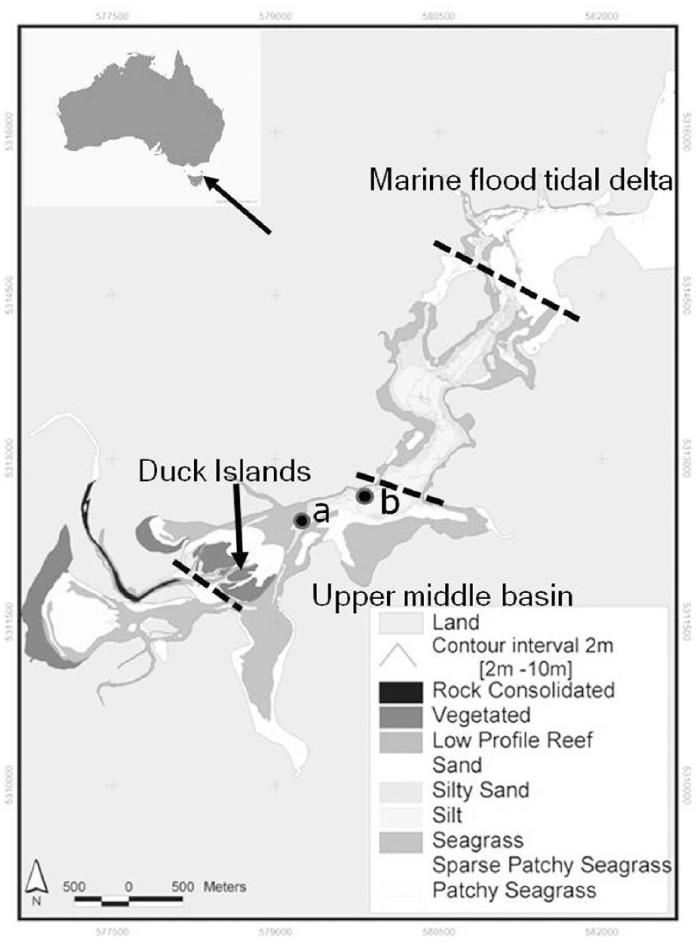
Sediment core sites (a) LSPMB2B08 and (b) LSPMB206 within the Little Swanport River Estuary (42.33°S, 147.98°E), a distinctive biological region (see text) located at the upper middle basin. The light grey regions represent seagrass meadows, and the dark grey regions represent saltmarsh.

Methods

Sediment cores were collected using a sliding hammer Kajak corer (UWITEC, Austria) equipped with a 6-cm internal diameter polycarbonate core tube. Sediment samples for ²¹⁰Pb dating and ¹⁴C dating of major shell deposits (shell carbonate) were chemically processed and measured at the Australian Nuclear Science and Technology Organisation (ANSTO). (For full details of sample processing, see Gallagher (2013).)

A number of partial tautological potential flood proxies were chosen. All the proxies were consistent with a high-energy environment as discontinuities from a perceived baseline and/or a spike in the supply of material from the upper estuary littoral regions and/or catchment soils. It was anticipated that each proxy would have its strengths and weaknesses, that is, different signal-to-noise ratios, sensitivities and assumptions, for a range of flood depositional components. Consistency with a flood event was supported as likely from the convergence of at least two centrist positions of discontinuity and/or upper and lower depositional facies boundaries on a case-by-case basis. Traditional data compression and classification methods, such as cluster and principal component analysis, were not effective. Sedimentary variables produced overlapping similarities between and across clearly plausible baseline sediments within plausible flood facies, for example, larger shell masses (see the ‘Results and discussion’ section).

Flood proxies

Catchment soils washed in by floods and loaded with terrestrial plant material were expected to have a smaller particulate atomic organic nitrogen to organic carbon (ON/OC) ratio and a lighter ¹³C_org (typically ±0.08) over estuarine sediments supporting seagrass, macroalgae and microalgae. Total organic nitrogen to organic carbon (TN/OC, standard error (SE) ±0.005) and stable organic carbon isotope (¹³C_org, SE ±0.08‰) ratios were measured at the West Australian Biogeochemistry Centre, University of Western Australia. TN was corrected to ON by subtracting the ammonia sorption from the intercept with the OC relationship (Gallagher, 2013). All ¹³C_org values were corrected for the Suess effect (Schelske and Hodell, 1995). Relatively low total organic matter (OM) content, CaCO₃ and water contents associated with fluvial silts/sands found in shell laden littoral and intertidal environments were measured as loss on ignition (LOI_550°C and LOI_950°C, SE ±0.08% and ±0.13%, respectively) and evaporation (105°C ± 0.1%), respectively (Heiri et al., 2001). Spikes in total iron content (SE ±0.001%) were measured in the upper sediment core (Box, 1984), consistent with the occurrence of the fluvial sediments supplied from upper catchment iron-laden pyroxene clays. This was supported by the obvious formation of yellow ash over usually brick red residue seen after sediment combustion at 950°C in both the upper and lower sediment cores. Tests indicated that this was the result of pyroxene clays reacting in the presence of shell CaCO₃ (Gallagher, 2013). Abiotic residual detritus content, that is, all biogenic contents removed from the total weight (LOI_550°C, CaCO₃ and biogenic silica (BSi; SE ±7.5%)), was used to more directly postulate an increase in fluvial supply.

Particle size distribution, and associated low OM and water content, typical of a flood’s high-energy environments, was evaluated as such through the presence of copepod faecal pellets in the same fluvial/silt size range (Dean et al., 2001). Copepods were not found during floods in the Little Swanport River Estuary (Crawford et al., 2005). In place of the time-consuming effort of counting pellets and sediment particles on sieves, faecal pellet presence was determined from a pattern analysis of OM across size fractions. The presence of a significant fraction of copepod faecal pellets was determined through a parallel variance between the OM content of the pellet’s size fraction and the OM content from the remains of the unpackaged fine fraction. In other words, the organic content of the faecal pellets should closely reflect the egested fine fraction in a way that the similarly sized fluvial silt fraction would not. Consequently, the absence of copepods and their faecal pellets in flood facies would result in a change from a positive correlation to an inverse correlation between faecal pellet fractions.

OM finger printing was conducted using simple furnace-based thermogravimetry. Detrital OM sources may be determined from the loss in weight across the higher combustion temperatures (280–520°C) to the total loss in weight between 135°C and 520°C (Kristensen, 1994). The ratio is known as the Rp index (SE ±0.01). This interpretation was modified to one in which an elevated Rp index above an apparent baseline was not only consistent with the presence of high freshwater humic acid content but was also the result of more efficient OM combustion because of the presence of calcium carbonate and structural water loss from pyroxene clays (Gallagher, 2013). The final interpretation was constrained by the presence or absence of the other component proxies.

Shell deposits were identified for poor habitat fidelity from upper estuarine and/or intertidal to supra-tidal zones (Grove, 2017). The temporal shell fidelity with respect to the Anthropocene was measured from the ¹⁴C of the shell carbonate from the largest and dominant species (ANSTO). Macro char deposits were prepared and counted according to Rhodes (1998) as within baseline sediment markers of recorded pivotal fires. Further details of all analytical and sampling methods can be found in Gallagher (2013).

Flood geochronology

The flood event chronology was constructed by correlating the largest set of flood events from the present to the past, between 1900 and 2001, and more contemporary records of river flow, from a re-analysis of a calibrated rainfall/river flow catchment and land-use model (SKM, 2004). The largest set was matched to the flood facies from the present to the past in relation to an apparent common signal size as coring did not capture the whole facies at the bottom of the cores. Any inability to match the flood facies/signals to the larger flood sets was noted, and the reason for it was hypothesised in relation to a core with a successful correlation.

Erosion and ²¹⁰Pb geochronologies

The extent of erosion was assessed only on cores that showed direct evidence in baseline sediments from a deficit from expected atmospheric supply in ²¹⁰Pb. In other words, the measured excess ²¹⁰Pb inventory, from an integration that excluded the ²¹⁰Pb values within the flood facies, was less than the calculated atmospheric supply inventory for south-east Tasmania (Turekian et al., 1977). The quantity and placement of erosion were then solved iteratively by increasing the eroded accumulative mass, consecutively to regions below the flood facies and in direct proportion to the strength of the flood. A solution was reached when the total ²¹⁰Pb inventory became equal to the inventory calculated from the atmospheric supply for south-east Tasmania. The thickness of the eroded sediment was then calculated from the average dry bulk density of the surrounding baseline horizons. Finally, the SIT, CRS and CIC geochronologies were calculated on the reconstructed baseline sediment column, which is the amount added from erosion below the flood facies minus the flood facies. For details of CRS and CIC calculations, see Oldfield and Appleby (1984). For SIT, we used the algorithmic procedure of Liu et al. (1991) with software kindly provided by Dr Carroll.

Results and discussion

Sediment core descriptions for LSPMB206

The top 2 cm of the 75-cm sediment core at LSPMB206 had the colour and consistency of olive green to black anoxic mud, with a faint smell of sulphide. Dispersed throughout the core were well-preserved pieces of Zostera seagrass leaves. The length of the leaf debris ranged from a few millimetre to around 2 cm. Between 28 and 35 cm and 62 and 75 cm, there were two notable masses of shells and shell debris in a sandier black matrix. The shells within the intrusive masses consisted of gastropods and molluscs, notably, the bivalve Spisula trigonella, up to 4 cm in length. The shells were not sufficiently evenly dispersed to mark the borders of the facies with any precision. Outside the shell masses, an occasional small whole or piece of gastropod or mollusc shell a few millimetre in diameter was found dispersed throughout most of the sediment core.

All of the habitats of the shell species were more typical of sub-tidal to intertidal regions of a muddy estuary (Table 1) and thus likely to have been washed in by a flood event. Furthermore, the ¹⁴C age of the Spisula trigonella shells in the two major facies, at 503–791 yr BP, was much older than the presence of excess ²¹⁰Pb activity would suggest, that is, <150 years (see Figure 6). The suggestion is that the shells were likely to have come from the nearby shell middens (Sloss et al., 2007).

Table 1.

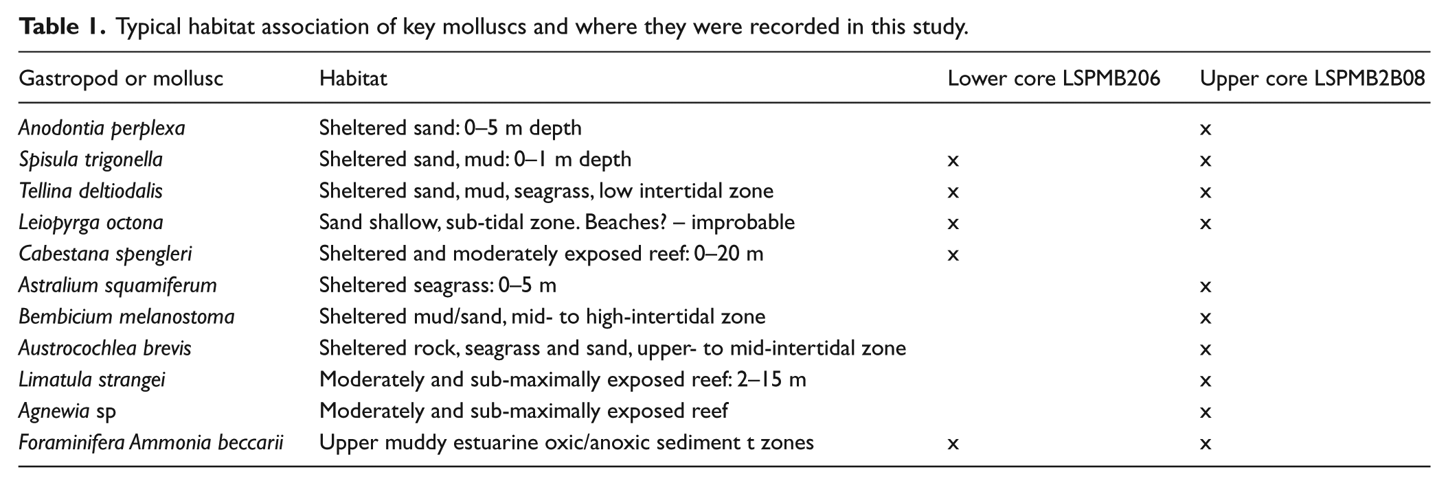
Typical habitat association of key molluscs and where they were recorded in this study.

Gastropod or mollusc	Habitat	Lower core LSPMB206	Upper core LSPMB2B08
Anodontia perplexa	Sheltered sand: 0–5 m depth		x
Spisula trigonella	Sheltered sand, mud: 0–1 m depth	x	x
Tellina deltiodalis	Sheltered sand, mud, seagrass, low intertidal zone	x	x
Leiopyrga octona	Sand shallow, sub-tidal zone. Beaches? – improbable	x	x
Cabestana spengleri	Sheltered and moderately exposed reef: 0–20 m	x
Astralium squamiferum	Sheltered seagrass: 0–5 m		x
Bembicium melanostoma	Sheltered mud/sand, mid- to high-intertidal zone		x
Austrocochlea brevis	Sheltered rock, seagrass and sand, upper- to mid-intertidal zone		x
Limatula strangei	Moderately and sub-maximally exposed reef: 2–15 m		x
Agnewia sp	Moderately and sub-maximally exposed reef		x
Foraminifera Ammonia beccarii	Upper muddy estuarine oxic/anoxic sediment t zones	x	x

Sediment core stratigraphy for LSPMB206

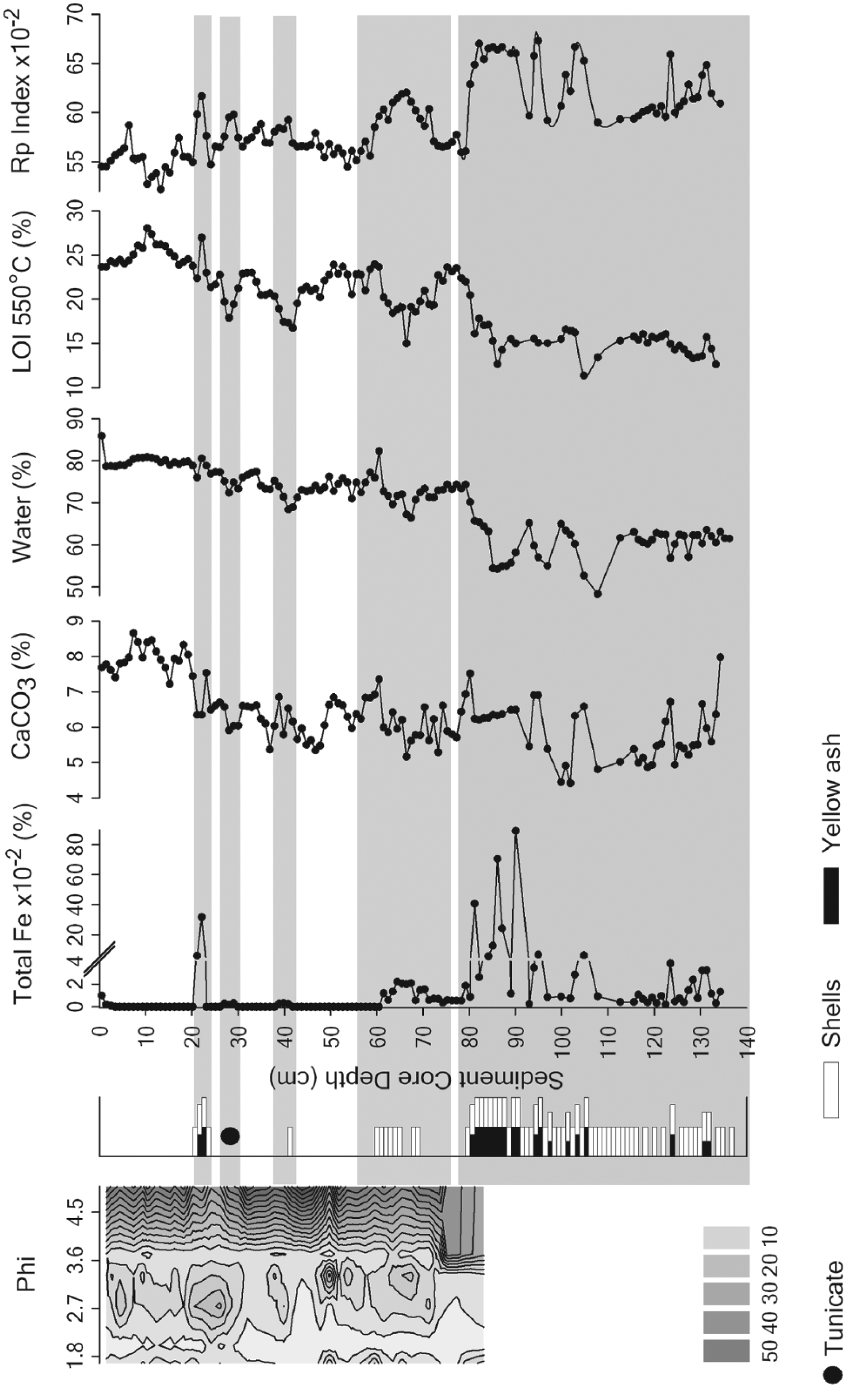
The grey bars across the depth stratigraphy in Figure 2 represent the positions and extent of flood proxy discontinuities from the perceived baseline trends, analysed after the fact. This is to assist in the comparisons between the variance of the content and quality variables. Overall, it was found that LOI_550°C, RD and water content had non-linear baseline trends. The troughs in LOI_550°C and the peaks in RD and water content were consistent with silty fluvial sediments and followed each other relatively closely but not in constant proportions. Indeed, the lack of evidence for copepod faecal pellets within the total and fine fraction (<76 µm) LOI_550°C troughs (Figure 3a) reaffirmed that the implied turbulent environment was likely associated with a flood (Crawford et al., 2005). That is, the divergence (i.e. loss in correlation) of the OM depth profiles between the total or fine fraction and the middle 150- to 100-µm size silt or faecal pellets fractions down the flood facies indicated that the middle fraction did not come from copepod feeding and egestion of the fine fraction particles. Surprisingly, peak discontinuities for CaCO₃ were not as clear and failed to increase in the presence of the bottom shell mass. It may have been the relative lack of shell hash that was responsible for the invariant CaCO₃ content profile.

Figure 2.

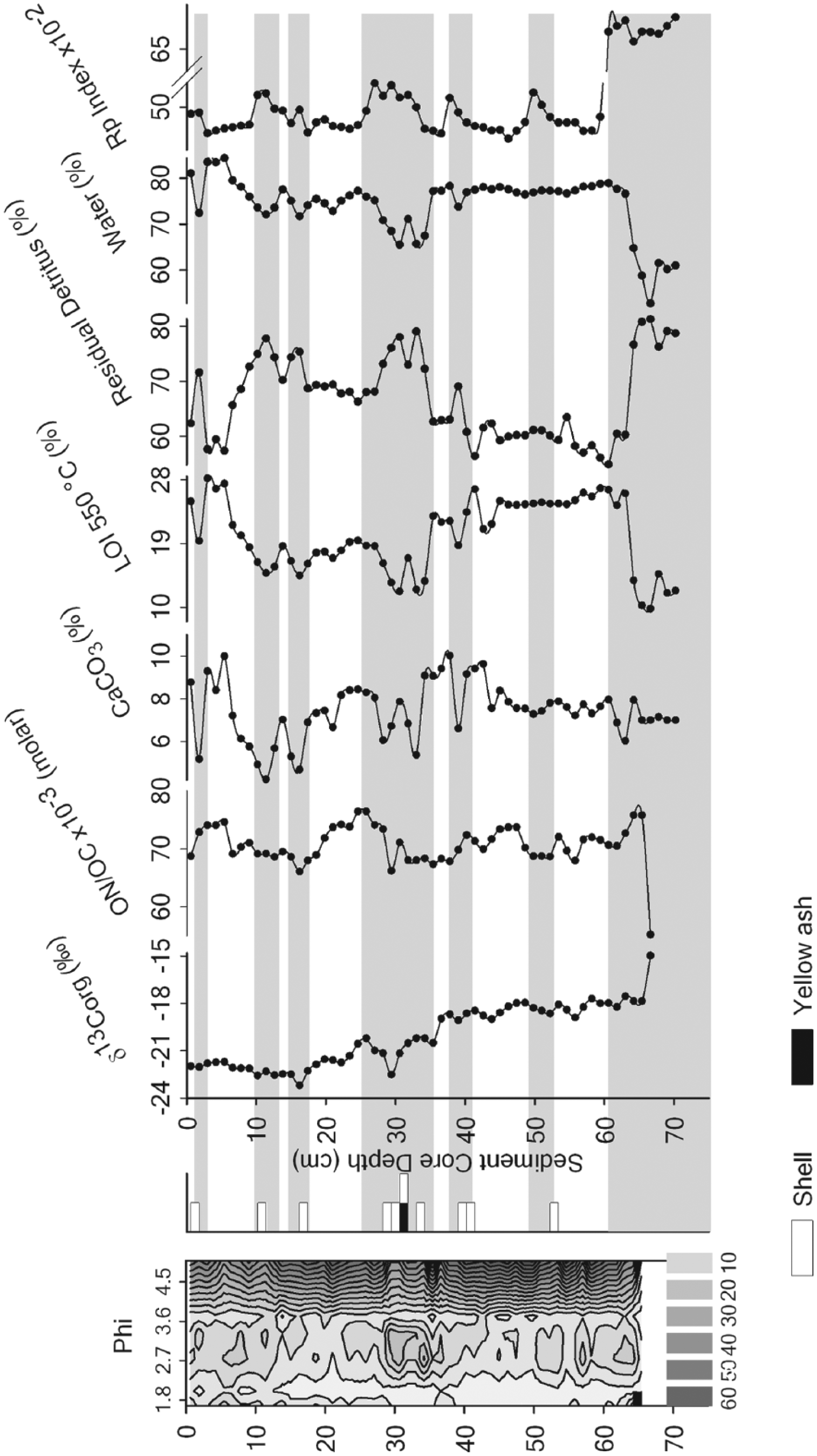
Content variables (% dry weight corrected for salt content), shells and spikes in pyroxene clays (yellow ash) down the Little Swanport River Estuary’s upper middle basin sediment core LSPMB206. The yellow ash appeared after high-temperature combustion of the sediment (950°C) and was identified as being due to the interaction of calcium carbonate and pyroxene clays (see text). Carbonate refers to LOI_950°C as CaCO3 confirmed only after acid addition and re-analysis (Gallagher, 2013). The particle size distribution was measured as phi from the size of the sieve. The key shows the percentage of size categories as phi.

Figure 3.

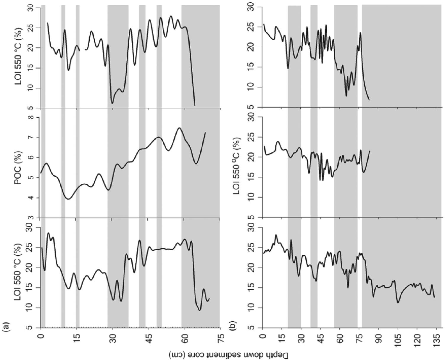
The OM content of sediment size fractions (% of dry weight corrected for salt content) down the Little Swanport River Estuary’s upper middle basin sediment cores (a) LSPMB206 and (b) LSPMB2B08; from left to right <76 μm, 100–150 µm and total. OM depth variance is expressed as either POC or LOI_550°C. The relative depth variance is used to infer the presence of faecal pellets (see text). The shaded areas represent deposits from high-energy events such as floods (see text for their assignments).

The δ¹³C_org and ON/OC profiles showed little correlation with each other or with the rest of the signal and content discontinuities (Figure 2). Both profiles had generically different baseline trends and/or deviations from their baselines. The δ¹³C_org profile remained relatively invariant down the sediment core to around 46 cm and was significantly heavier below 46 cm. The ON/OC profile displayed an apparent periodicity about a relatively invariant trend down the length of the core. Indeed, the capacity of δ¹³C_org–ON/OC duplet variance for detecting flood events as a light δ¹³C_org (typically >28‰) and low ON/OC (typically <0.04) was surprisingly poor. The poor association probably reflects the importance of flood remobilisation and re-deposition of littoral sediments over the deposition of catchment soils.

In contrast to the other proxies, the elevations in the Rp index appeared to remain on a stationary baseline of around 0.43 (Figure 2). With the exception of an extra elevation above baseline at around 49–53 cm, the Rp index was in agreement with the centrist positions of the other content discontinuities, although the shallower upper boundaries were not always coincident (e.g. at 25 and 61 cm). Nevertheless, discontinuity in the Rp index was the only proxy that overlapped the other content and quality discontinuities in ways consistent with flood deposition. In other words, high Rp index values were associated with the contents of high-energy silty sandy environments (Loh et al., 2008). However, the Rp index elevations around the apparent baseline stratigraphy were not always clear. The relatively small Rp index elevation (0.5) at 16 cm, though within error (see section ‘Methods’), could arguably be the result of a stochastic outlier. Furthermore, the boundaries that mark the elevations were not always the same as other content variable peaks or troughs, for example, the shallower upper boundary indicated by the water content and RD of the major larger bottom and middle facies and the shallower lower boundary of the larger middle facies. Furthermore, the Rp index elevation between 49 and 53 cm was only coincident with one other weak signal, namely, the presence of a single gastropod shell near the border of its deeper boundary. A high freshwater particulate humic acid content is the most likely explanation for the elevated Rp index, given that it was coincident with the fall in the ON/OC ratio, typical of humic acids (Kristensen, 1990). Significant inputs of humic acids can be supplied to the estuary with strong flows and floods as they flocculate near the freshwater/seawater interface located at the base of the salt wedge (Karbassi et al., 2008).

In summary, overall, the elevation of Rp index when referenced to an apparent baseline, with relatively little white noise across its stratigraphy, appears to be the best candidate for a universal flood event marker for this lower sediment core, although, on occasion, the index may require additional support where the peaks are small relative to the baseline noise. This might include support from the presence of shells and animals, yellow ash from high-temperature combustion (i.e. pyroxene clays in the presence of calcium carbonate) or other proxy discontinuities with greater signal-to-noise ratios, such as RD, LOI_550°C and water content.

Sediment core descriptions for LSPMB2B08

The top 4 cm of the core was of a similar olive green colour to the anoxic surface sediments of core LSPMB206. However, a faint smell of sulphide was detected deeper down the core at around 5–12 cm. Similar to core LSPMB206, well-preserved pieces of seagrass leaves were dispersed throughout the sediment core, but in obviously greater abundance. In addition, the remains of a piece of well-preserved red to orange freshwater tunicate of around 2 cm in diameter were also found, but with no evidence of shell debris (Figure 4). The size of the tunicate relative to the size of the depositional facies at this particular coordinate may well have excluded the shell debris seen in near adjacent parts of the sediment column.

Figure 4.

Content variables (% dry weight corrected for salt content), shells and total iron down the Little Swanport Estuary’s upper middle basin sediment core LSPMB2B08. The yellow ash refers to the sediment appearance after high-temperature combustion (950°C) in the presence of CaCO₃ and iron-laden pyroxene clays. Carbonate refers to LOI_950°C as CaCO₃ confirmed only after acid addition and re-analysis (Gallagher, 2013). The contours represent particle size distribution from sieves as phi. The key gives the percentage of size categories as phi. The grey bars are the suggested positions of flood facies (see text for assignments).

The upper sediment core, like the lower sediment core, contained large shell masses but at different depths: 20–25, 59–75 and 80–134 cm (Figure 4). The shell assemblage was dominated by relatively large numbers of the bivalve Spisula trigonella (up to 3 cm long) and Tellina deltiodalis (up to 5 cm long). In general, in the lower site, the shell fidelity was poor (associated habitats were sub-tidal to intertidal), but with a more diverse mix of gastropods and molluscs (Table 1). Again, in the upper core site, shells were not always evenly dispersed throughout the masses; nevertheless, they appeared to be more ubiquitous.

Sediment core stratigraphy for LSPMB2B08

Both the upper and lower sediment cores had similar ranges of CaCO₃, LOI_550°C and water content: 4.4–8.7%, 11.3–28.0% and 48.3–85.8%, respectively (Figure 4). However, the baseline Rp indexes found down the core (at around 0.53) were significantly larger than those found down core LSPMB206 (around 0.45) despite similar maximum values at the deepest discontinuities (around 56–78 and >80 cm) associated with the shell masses of 0.68 and 0.69, respectively. This probably reflects a general maximum of this signal for sediments. For the most part, the major content profiles and the Rp index profile were noisier than those for LSPMB206. In particular, the depth profile of the CaCO₃ content –signal-to-noise ratio was too large for any definitive identification of peaks or troughs.

Overall, the peaks in iron content and the Rp index, with the exception of the surface-elevated iron content, converged down the sediment core (Figure 4). It is probable that the surface iron content was the result of iron redox remobilisation and precipitation immediately above the anoxic/oxic interface (Davison and Heaney, 1978). The relative peaks in iron content within the largest intrusive shell mass (>80 cm) were more variable than the Rp index, and they were always accompanied by the appearance of yellow ash, found to be formed during high-combustion temperatures in the presence of CaCO₃ (Gallagher, 2013). Interestingly, there was no yellow ash in the presence of smaller iron content (<0.04% dwt) centred around 40 cm and the shell mass between 56 and 78 cm. The reason for this lack of consistency was not clear. It is possible that the iron was from another source, perhaps associated with humic acid flocs formed at the bottom of a salt wedge (Karbassi et al., 2008).

As in the lower core, large troughs in water content and LOI_550°C ostensibly followed the elevated Rp index regions and, at times, had a clearer signal-to-noise ratio (Figure 4). The exception was a small but significant contiguous asymmetrical elevation in the Rp index centred at 37 and 40 cm but matched by a large water content or LOI_550°C variance. Together with a relatively small elevated iron content, this confirmed the presence of a relatively small elevated Rp index at that depth. The elevated Rp index at 37 cm, however, was not supported by other variable discontinuities consistent with high-energy environments. In contrast, the clearer and larger Rp index and iron peak around 24 cm provided strong evidence of a flood event. However, there was no significant change in LOI_550°C or water content, other than a change to a profile that was noisier than the shallower profile. The reasons for such a decoupling from LOI_550°C and water content are unclear. We suggest that the decoupling is the result of an additional contribution to the water content and OM from the presence of fully hydrated seagrass leaf detritus.

As in the lower sediment core, the boundaries could also be discerned from the divergence between the fine fraction’s OM and the OM within the sand/faecal pellet fractions (Figure 3b). The profiles show divergence between the fine fraction and the faecal pellet/sand fraction down the two bottom notable masses from around 56 to 74 cm and >78 cm. The latter was separated by 3–4 cm of baseline sediment and was consistent with the variance in the Rp index. This observation alone indicates that the depositional facies was not likely to be the same contiguous deposit despite the greater structural variability in other content variables (e.g. total iron and CaCO₃). However, the pattern resolution was not sufficient to separate the two high-energy discontinuities between 22 and 31 cm. Nevertheless, the pattern was sufficient to resolve the remaining high-energy discontinuity (around 40 cm) as a notable switch to an inverse correlation with both the total LOI_550°C and the LOI_550°C of the fine fractions.

Flood fire event geochronology

The modelled flood events were successfully matched to the magnitude and sequence of the Rp index signal, as well as to the facies thickness down sediment core LSPMB206 (Figure 5). The 1969 and 1970 flood events were pooled as one facies, as they were separated by 2–3 months, a time too short to separate as depth down the core. Nevertheless, this correlation could be considered robust. The sequence remained correlated with the two significantly larger floods of the 20th century (1923 and 1960) with two clearly identifiable, significantly larger facies down the sediment core. In addition, the largest macro char peak was well positioned between flood events with the largest fire recorded within south-east Tasmania in 1967 (Black Tuesday).

Figure 5.

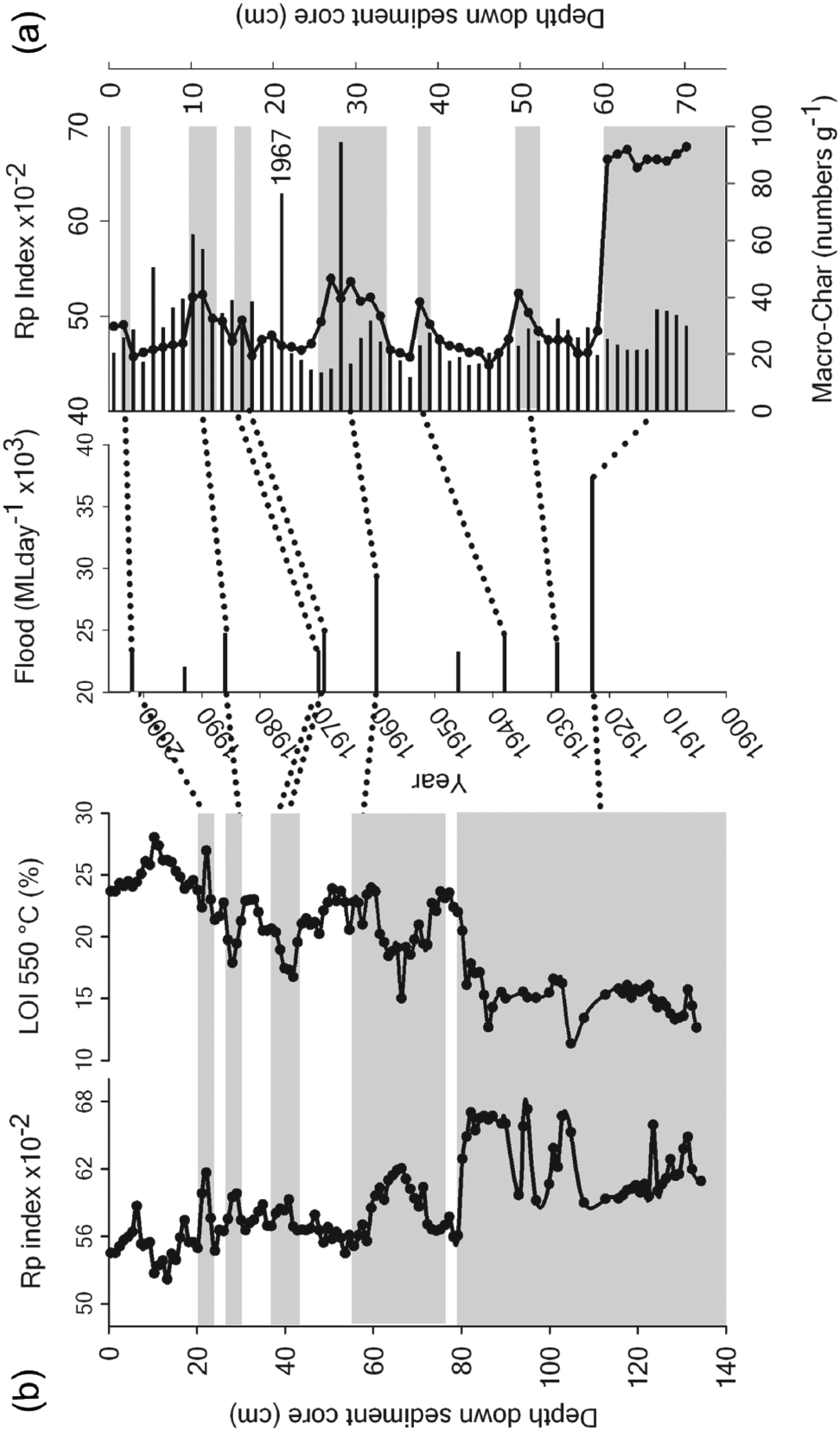
Flood event geochronologies down the Little Swanport River Estuary’s upper middle basin sediment cores (a) LSPMB2B08 and (b) LSPMB206. The relative event magnitudes within the sediment core are represented by the thicknesses of the event facies and the magnitude of the Rp index for sediment core LSPMB206, in combination with LOI_550°C for sediment core LSPMB2B08.

The correlation between the flood and its event facies down upper sediment core LSPMB2B08 was not as clear. This was, in part, because neither the magnitude of the Rp index signal alone nor the other content variables reflected the thickness of all the facies (Figure 5). However, using the Rp index in combination with LOI_550°C, there was sufficient commonality and overlap between all three metrics to match flood events to their facies. Nevertheless, a solution was only possible by assuming that the two larger intrusive masses represented the 1960 and 1923 flood events and that the flood facies between these events had been eroded by the 1960 flood.

²¹⁰Pb contiguous geochronology

Figure 6 shows the ²¹⁰Pb activity depth profiles down the upper and lower cores before correcting depths for erosion and conceptually removing flood facies. At first glance, it seems that the profile shape more or less decreases with depth. These are conditions that appear not to violate, at least one criterion for CRS and CIC mapping procedures. An increase in ²¹⁰Pb activity with depth implies a negative sedimentation rate or a decrease in sediment age with depth. However, the ²¹⁰Pb profile alone cannot distinguish between increases in sedimentation and ²¹⁰Pb supply, nor can we assume that flood deposits are old catchment soils with no excess ²¹⁰Pb activity (Arnaud et al., 2002; Drexler and Nittrouer, 2008), which would otherwise be detected down the sediment core. For many bar-built estuaries, this concept is misleading, as they are subjected to deposition from and younger littoral sources (see the ‘Introduction’ section).

Figure 6.

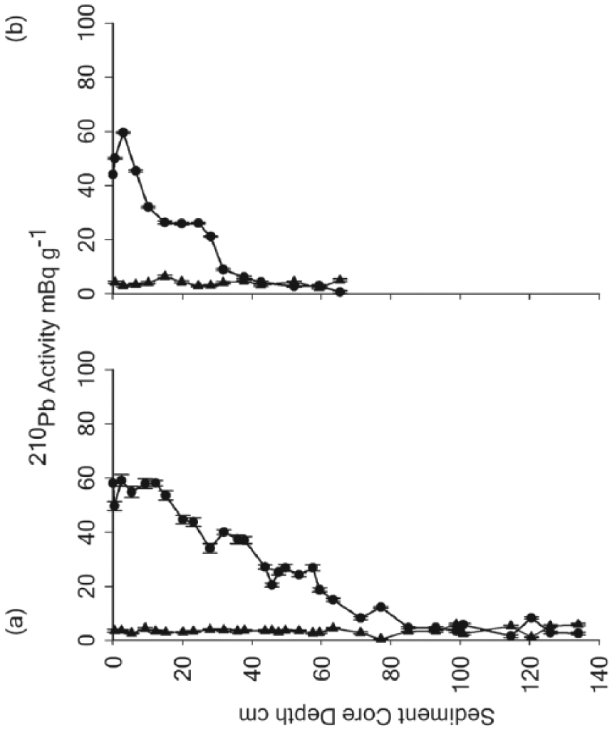
²¹⁰Pb activity (as per dry weight corrected for salt content) down the Little Swanport River Estuary’s sediment cores (a) LSPMB2B08 and (b) LSPMB206. Unsupported ²¹⁰Pb activity (●) and ²¹⁰Pb supported fraction (▲). The error bars are standard deviations of the decay counts.

When the flood facies had been conceptually removed to leave model ²¹⁰Pb depth baseline profiles (Arnaud et al., 2002), only the lower core, LSPMB206, showed direct evidence of erosion. The excess ²¹⁰Pb baseline sediment inventory of 2260 Bq m⁻²) was significantly less than expected from local aerial deposition, as 3363 Bq m⁻² (Turekian et al., 1977). In contrast, the baseline sediment excess ²¹⁰Pb inventory for the upper core, LSPMB2B08 of 4990 Bq m⁻², remained considerably larger than that supplied solely from aerial deposition. The result likely indicates that there was considerably more ²¹⁰Pb supplied to the site, rather than it was less subjected to erosion. The upper core flood event chronology showed evidence consistent with the loss of two flood facies and a proportionally greater loss of baseline sediments between the remaining facies (see the ‘Flood fire event geochronology’ section). The source of the extra ²¹⁰Pb supply is likely from catchment soils and fluvial sediments, littoral zone sediment focusing and/or erosion from the nearby depositional levees (Figure 1).

The SIT, CIC and CRS models and methods were also applied to the complete sediment column for the upper core (see the ‘Methods’ section for justification). Indeed, there was general agreement with all ²¹⁰Pb models and the flood event chronology for the lower core site, LSPMB206 (Figure 7b). The agreement across the lower core suggests a relatively constant flux of ²¹⁰Pb from the atmosphere, at times, with a varying baseline sedimentation rate. There were varying degrees of agreement between the horizon dates and the flood facies throughout the sediment core. Nevertheless, overall, the SIT model remained the most accurate, with the possible exception of the 1923 flood event (Figure 7b). This was in contrast to the CIC horizon dates, which closely matched the 1923 flood event but exhibited greater divergence within the upper and middle core sections (Figure 7b). Conversely, the CRS method underestimated the event age towards the top of the sediment core but diverged towards an older estimation of the remaining flood events towards the bottom of the sediment core (cf. SIT in Figure 7b).

Figure 7.

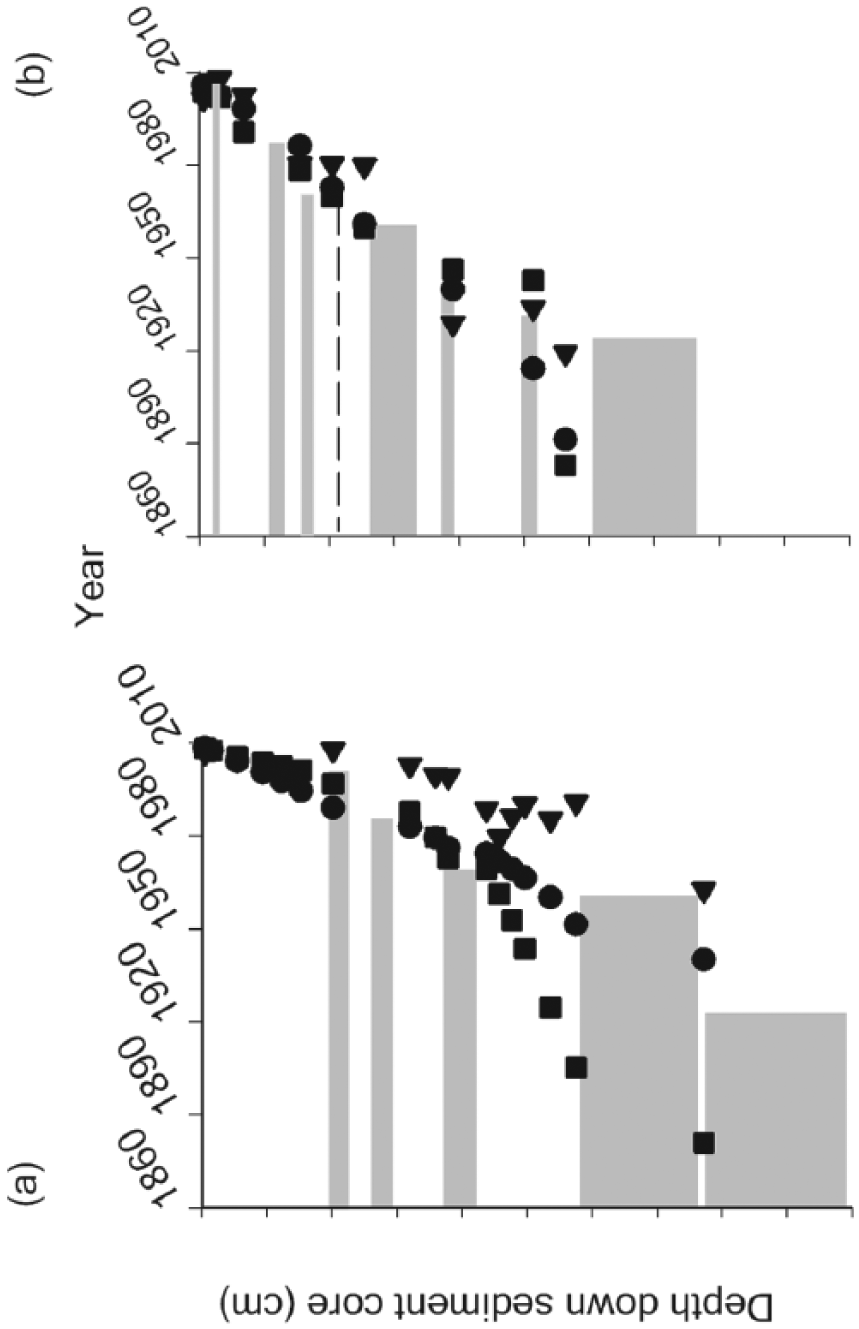
Comparison of flood events and ²¹⁰Pb geochronologies, CIC (▲), CRS (●) and SIT (■), for the Little Swanport River Estuary’s upper middle basin sediment cores (a) LSPMB2B08 and (b) LSPMB206. The black dotted line marks the 1967 fire (b) and the grey bars mark the positions and age of river flood depositional facies.

In contrast to sediment core LSPMB206, there was no convergence between any of the radio-geochronological methods and events down sediment core LSPMB2B08, despite an increased sampling resolution (Figure 7a). The inability to correct and assess whether there was erosion, however, was only partly responsible for the divergence between the separate geochronologies. The CIC baseline horizons (independent of erosion) did not match any of the event dates, with the possible exception of the 2001 flood (Figure 7a). The disagreement suggests a complex relationship between the sedimentation rate and the supply of excess ²¹⁰Pb, which violated CIC assumptions. The disagreement also highlights that an independent evaluation throughout the sediment column is essential, given that the SIT model fit to the profile was good and that early events (the 2001 flood) should show an approximate convergence with the CRS and CIC methods (Figure 7a).

Conclusion

The results show that it is possible to produce a sediment column for a ²¹⁰Pb contiguous late Anthropocene geochronology and an accretion profile in flood-affected bar-built estuaries and lagoons, despite variability in flood remobilisation signals and without a priori knowledge of the amount of flood erosion. However, for the construction and evaluation of a flood event chronology, more than one plausible sampling site and commonly available or constructed rainfall/river fall long-term data sets are required.

Lessons taken from the Little Swanport River Estuary suggest that other systems will likely show multiple depositional flood facies and evidence of flood erosion throughout the late Anthropocene. For the Little Swanport River Estuary, depositional flood events appeared to have occurred when floods were >23,200 mL day⁻¹. For other systems, the frequency will depend on the size of the river flows relative to the estuarine volume to produce a velocity sufficient to remobilise and deposit sediments. Finally, constructing such a geochronological set will allow researchers to successfully tackle dynamic non-ideal depositional environments, which are the norm in many of these systems. This may lead to a more complete understanding of their long-term ecosystem dynamics, from pressed factors, events and the role historical contingency, at their seascape scales.

Footnotes

Funding

This programme was support by funds supplied by the Hub, Landscape Logic (University of Tasmania) and Australian Nuclear Science and Technology Organisation (ANSTO) at Lucas Heights, Sydney (AINARA 07166 and private project number 2009rc11abc).

References

Abril

(2004) Constraints on the use of Cs-137 as a time-marker to support CRS and SIT chronologies. Environmental Pollution 129: 31–37.

Abril

(2015) Why would we use the Sediment Isotope Tomography (SIT) model to establish a 210Pb-based chronology in recent-sediment cores? Journal of Environmental Radioactivity 143: 40–46.

Abril

Brunskill

(2014) Evidence that excess 210Pb flux varies with sediment accumulation rate and implications for dating recent sediments. Journal of Paleolimnology 52: 121–137.

Appleby

(2001) Chronostratigraphic techniques in recent sediments. In: Smol

Last

(eds) Tracking Environmental Change Using Lake Sediments: Terrestrial, Algal and Siliceous Indicators. Dordrecht: Kluwer Academic Publishers, pp. 171–203.

Arnaud

Lignier

Revel

et al . (2002) Flood and earthquake disturbance of Pb-210 geochronology (Lake Anterne, NW Alps). Terra Nova 14: 225–232.

Barbier

Hacker

Kennedy

et al . (2011) The value of estuarine and coastal ecosystem services. Ecological Monographs 81: 169–193.

Box

(1984) Observations on the use of iron (ii) complexing agents to fractionate the total filterable iron in natural water samples. Water Research 18: 397–402.

Bycroft

(2010) Going outside the model: Robustness analysis and experimental science. Spontaneous Generations 3: 123–141.

Carpenter

Leavitt

(1991) Temporal variation in a paleolimnological record arising from a trophic cascade. Ecology 72: 277–285.

10.

Carroll

Lerche

Abraham

et al . (1999) Sediment ages and flux variations from depth profiles of Pb-210: Lake and marine examples. Applied Radiation and Isotopes 50: 793–804.

11.

Cooper

JAG

(2002) The role of extreme floods in estuary-coastal behaviour: Contrasts between river- and tide-dominated microtidal estuaries. Sedimentary Geology 150: 123–137.

12.

Crawford

Mitchel

(1999) Physical and Chemical Parameters of Several Oyster Growing Areas in Tasmania (Tech report series 155m). Hobart: Tasmanian Aquaculture and Fisheries Institute, University of Tasmania, pp. 1441–8487.

13.

Crawford

Neira

White

(2005) Environmental Flows In the Little Swanport Estuary. Hobart: Tasmanian Aquaculture and Fisheries Institute, University of Tasmania.

14.

Crutzen

(2002) Geology of mankind. Nature 415: 23.

15.

Davison

Heaney

(1978) Ferrous iron-sulfide interactions in anoxic hypolimnetic waters. Limnology and Oceanography 23: 1194–1200.

16.

De Groot

Brander

van der Ploeg

et al . (2012) Global estimates of the value of ecosystems and their services in monetary units. Ecosystem Services 1: 50–61.

17.

Dean

Kemp

AES

Pearce

(2001) Palaeo-flux records from electron microscope studies of Holocene laminated sediments, Saanich Inlet, British Columbia. Marine Geology 174: 139–158.

18.

Deflandre

Mucci

Gagne

et al . (2002) Early diagenetic processes in coastal marine sediments disturbed by a catastrophic sedimentation event. Geochimica et Cosmochimica Acta 66: 2547–2558.

19.

Donato

Reinhardt

Boyce

et al . (2009) Particle-size distribution of inferred tsunami deposits in Sur Lagoon, Sultanate of Oman. Marine Geology 257: 54–64.

20.

Drexler

Nittrouer

(2008) Stratigraphic signatures due to flood deposition near the Rhone River: Gulf of Lions, northwest Mediterranean Sea. Continental Shelf Research 28: 1877–1894.

21.

Elwany

MHS

Flick

Aijaz

(1998) Opening and closure of a marginal southern California lagoon inlet. Estuaries 21: 246–254.

22.

Engstrom

Wright

(1984) Lake Sediments and Environmental History: Studies in Palaeolimnology and Palaeoecology in Honour of Winifred Tutin (ed Haworth

Lund

JWG

). Leicester: Leicester University Press.

23.

Eyre

Twigg

(1997) Nutrient behaviour during post-flood recovery of the Richmond River Estuary Northern NSW, Australia. Estuarine Coastal and Shelf Science 44: 311–326.

24.

Foster

IDL

Mighall

Proffitt

et al . (2006) Post-depositional Cs-137 mobility in the sediments of three shallow coastal lagoons, SW England. Journal of Paleolimnology 35: 881–895.

25.

Gallagher

(2013) Natural and Anthropogenic Ecosystem Regime Variance within a Tide-Dominated Estuary: A Late Anthropocene Palaeo-Reconstruction. Hobart: Department of Zoology, University of Tasmania, p. 239.

26.

Grove

(2017) A Guide to the Seashells and other Marine Molluscs of Tasmania. Available at: http://www.molluscsoftasmania.net/index/html

27.

Habeeb

Johnson

Wotherspoon

et al . (2007) Optimal scales to observe habitat dynamics: A coral reef example. Ecological Applications 17: 641–647.

28.

Hancock

Pietch

(2006) Sedimentation in the Gippsland Lakes as determined from sediment cores. Report to the Gippsland Coastal Board, CSIRO Land and Water Science Report 40/06. Available at: http://citeseerx.ist.psu.edu/viewdoc/download;jsessionid=DC3DC4DE43F8E63038E8B915A8D18852?doi=10.1.1.520.653&rep=rep1&type=pdf

29.

Walling

(1996) Interpreting particle size effects in the adsorption of 137Cs and unsupported 210Pb by mineral soils and sediments. Journal of Environmental Radioactivity 30: 117–137.

30.

Heiri

Lotter

Lemcke

(2001) Loss on ignition as a method for estimating organic and carbonate content in sediments: Reproducibility and comparability of results. Journal of Paleolimnology 25: 101–110.

31.

Inkpen

Wilson

(2009) Explaining the past: Abductive and Bayesian reasoning. Holocene 19: 329–334.

32.

Karbassi

Nouri

Mehrdadi

et al . (2008) Flocculation of heavy metals during mixing of freshwater with Caspian Sea water. Environmental Geology 53: 1811–1816.

33.

Kirchner

Ehlers

(1998) Sediment geochronology in changing coastal environments: Potentials and limitations of the Cs-137 and Pb-210 methods. Journal of Coastal Research 14: 483–492.

34.

Kortekaas

Dawson

(2007) Distinguishing tsunami and storm deposits: An example from martinhal, SW Portugal. Sedimentary Geology 200: 208–221.

35.

Kristensen

(1990) Characterization of biogenic organic matter by stepwise thermogravimtery (STG). Biogeochemistry 9: 135–159.

36.

Kristensen

(1994) Decomposition of microalage, vascular plants and sediment detritus in seawater: Use of stepwise thermogravimetry. Biogeochemistry 26: 1–24.

37.

Liu

Carroll

Lerche

(1991) A technique for disentangling temporal source and sediment variations from radioactive isotope measurements with depth. Nuclear Geophysics 5: 31–45.

38.

Loh

Reeves

Harvey

et al . (2008) The fate of terrestrial organic matter in two Scottish sea lochs. Estuarine Coastal and Shelf Science 76: 566–579.

39.

Longmore

O’Leary

Rose

(1983) Caesium-137 profiles in the sediments of a partial-meromictic lake on Great Sandy Island (Fraser Island), Queensland, Australia. Hydrobiologia 103: 21–27.

40.

Matsumoto

(2005) Recent sedimentation rates derived from Pb-210 and Cs-137 methods in Ise Bay, Japan. Estuarine Coastal and Shelf Science 65: 83–93.

41.

McGowan

Leavitt

Hall

et al . (2005) Controls of algal abundance and community composition during ecosystem state change. Ecology 86: 2200–2211.

42.

Oldfield

Appleby

(1984) Empirical testing of ²¹⁰Pb-dating models for lake sediments. In: Haworth

Lund

JWG

(eds) Lake Sediments and Environmental History: Studies in Palaeolimnology and Palaeoecology in Honour of Winifred Tutin. Leicester: Leicester University Press, pp. 93–124.

43.

Rhodes

(1998) A method for the preparation and quantification of microscopic charcoal from terrestrial and lacustrine sediment cores. The Holocene 8: 113–117.

44.

Robbins

Edgington

Kemp

ALW

(1978) Comparative 210-Pb, 137-Cs, and pollen geochronologies of sediments from Lakes Ontario and Erie. Quaternary Research 10: 256–278.

45.

Rustomji

(2007) Flood and drought impacts on the opening regime of a wave-dominated estuary. Marine and Freshwater Research 58: 1108–1119.

46.

Rustomji

Bennett

Chiew

(2009) Flood variability east of Australia’s Great Dividing Range. Journal of Hydrology 374: 196–208.

47.

Schelske

Hodell

(1995) Using carbon isotopes of bulk sedimentary organic matter to reconstruct the history of nutrient loading and eutrophication in Lake Erie. Limnology and Oceanography 40: 918–929.

48.

Short

Carruthers

Dennison

et al . (2007) Global seagrass distribution: A bioregional model. Journal of Experimental Marine Biology and Ecology 350: 3–20.

49.

SKM (2004) Little Swanport River Catchment – Water Balance Model and Scenario Assessment (ed DPIW). Armadale: DPIW.

50.

Sloss

Murray-Wallace

Jones

(2007) Holocene sea-level change on the southeast coast of Australia: A review. The Holocene 17: 999–1014.

51.

Smith

(2001) Why should we believe Pb-210 Sediment geochronologies? Journal of Environmental Radioactivity 55: 121–123.

52.

Strayer

Glitzenstein

Jones

et al . (1986) Long Term Ecological Studies: An Illustrated Account of Their Design, Operation, and Importance to Ecology. Millbrook, NY: Occasional Publication of the Institute of Ecosystem Studies.

53.

Suess

(1978) Distinction between Natural and Anthropogenic Materials in Sediments (Biogeochemistry of Estuarine Sediments). Melreux: UNESCO/SCOR, pp. 224–237.

54.

Turekian

Nozaki

Benninger

(1977) Geochemistry of atmospheric radon and radon products. Annual Review of Earth and Planetary Sciences 5: 227–255.

55.

Van Rijn

(2013) Simple general formulae for sand transport in rivers, estuaries and coastal waters. Available at: www.leovanrijn-sediment.com

56.

Wan

Chen

et al . (2004) The coupling relation between Pb-210(ex) and organic matter in sediments of enrichment nutrient lake: An example from Lake Chenghai, China. Geochimica et Cosmochimica Acta 68: A397.

57.

Whitlock

Larsen

(2001) Charcoal as a fire proxy. In: Smol

Birks

HJB

Last

(eds) Tracking Environmental Change Using Lake Sediments: Terrestrial, Algal and Siliceous Indicators. Dordrecht: Springer, pp. 75–97.

58.

Wiens

Milne

(1989) Scaling of ‘landscapes’ in landscape ecology, or, landscape ecology from a beetle’s perspective. Landscape Ecology 3: 87–96.

Sediment geochronology for bar-built estuaries subject to flood deposition and erosion: A robust multiproxy approach across an estuarine zone

Abstract

Keywords

Introduction

Study site

Methods

Flood proxies

Flood geochronology

Erosion and 210Pb geochronologies

Results and discussion

Sediment core descriptions for LSPMB206

Sediment core stratigraphy for LSPMB206

Sediment core descriptions for LSPMB2B08

Sediment core stratigraphy for LSPMB2B08

Flood fire event geochronology

210Pb contiguous geochronology

Conclusion

Footnotes

Funding

References

Erosion and ²¹⁰Pb geochronologies

²¹⁰Pb contiguous geochronology