Long-chain alkenone-inferred temperatures from the last deglaciation to the early Holocene recorded by annually laminated sediments of the maar lake Sihailongwan,northeastern China

Abstract

Abrupt temperature changes during the last deglaciation are well recognized in Greenland ice cores and in deep-sea sediment records. On the continent of monsoonal Asia, however, only a few terrestrial temperature reconstructions extend to the Younger Dryas (YD). This hampers the understanding of how the Asian monsoon system responded to large-scale boundary changes in ice-sheet dynamics and reorganizations of atmospheric–oceanic circulation between the last deglaciation and the Holocene. Here, we report an alkenone-inferred temperature record from varved sediments of the maar lake Sihailongwan, northeastern China. Alkenone provides temperatures that represent the water temperature during the growing season when the lake is ice-free. Annually laminated sediments provide a reliable time control. Reconstructed temperatures reveal a distinctive pattern of variations during the last deglaciation: a temperature increase of 6°C at the onset of the Bølling–Allerød, two cold intervals (during the Older Dryas and the intra-Allerød cold period), a relatively minor temperature decrease of 1–3°C during the YD, and a rapid temperature increase of 4–5°C at the early Holocene. The reconstructed temperature records from Lake Sihailongwan and adjacent regions indicate that summer (or growing season) temperature changes were smaller than is evident in Greenland ice core records that are weighted toward winter.

Keywords

annually laminated sediment early Holocene long-chain alkenone-inferred temperatures maar lake Sihailongwan varve chronology Younger Dryas

Introduction

The last deglaciation is of significant interest because the climate of the Northern Hemisphere experienced several distinct changes: the cold Oldest Dryas (OD), the Bølling–Allerød (BA) warm phase, and the Younger Dryas (YD) cold event. Isotopic ratios of oxygen and nitrogen indicate large amplitude temperature changes during the last deglaciation (Alley, 2000; Buizert et al., 2014). However, recent studies have indicated that temperature records from Greenland ice cores were highly weighted toward the winter season, with a very large cooling in winter compared with summer during the YD (Buizert et al., 2014; Denton et al., 2005). Modeling experiments show that winter ice edge displacements produce temperature changes that are consistent with Greenland ice core records, whereas summer ice edge displacements have a less significant temperature effect (Li et al., 2005). This supported a hypothesis that some abrupt paleoclimatic events were most likely winter phenomena (Buizert et al., 2014; Denton et al., 2005).

In the Asian monsoon region, however, only a few quantitative temperature reconstructions extend to the YD, and this hampers our ability to understand monsoon changes on a large spatial scale since a regional record may not be representative of an entire hemisphere. Although well-dated stalagmite δ¹⁸O records from monsoonal Asia reveal distinct hydrological changes during the last deglaciation, they cannot be considered as are not paleotemperature time series. Published paleotemperature reconstructions for the Asian monsoon region reveal asynchronous or less distinct temperature changes than they are observed in the northern Atlantic. For example, a pollen record from Lake Suigetsu exhibits asynchronous changes with a temperature decrease of 2–4°C between 12.30 and 11.25 cal. ka BP (Nakagawa et al., 2003). Pollen-based temperature reconstructions from both southern (Xiao et al., 2014) and northern China (Wu et al., 2016) indicate only a minor temperature decrease during the YD. A recent long-chain alkenone (LCK)-inferred temperature record from Lake Qinghai indicated only a minor temperature decrease during the YD (Hou et al., 2016). The lack of quantitative temperature records is a problem for climatic modeling and hampers us to understand how the Asian monsoon system responded to large-scale boundary changes in ice-sheet dynamics and the reorganizations of atmospheric–oceanic circulation between the last deglaciation and the Holocene.

Temperature-dependent lipids, LCKs, have been suggested as a quantitative paleotemperature indicator for lake sediments (Hou et al., 2016; Li et al., 2015; Liu et al., 2011; Pearson et al., 2008; Theissen et al., 2005; Theroux et al., 2013; Zhao et al., 2013). Many independent laboratory culture experiments (D’Andrea et al., 2016; Longo et al., 2016; Pearson et al., 2008; Sun et al., 2007; Toney et al., 2010) have confirmed that the concentrations of LCKs largely depend on the water temperature due to a biological mechanism that enables certain algae to maintain the viscosity of their internal fluids by adjusting the relative abundance of their lipids in response to changing ambient temperature. Nonetheless, the application is still largely empirical because of the high diversity of the alkenone precursor organisms, strong seasonal variability of algal assemblages, nonlinear relationship at low or high temperatures, or extreme conditions (e.g. Longo et al., 2016; Nakamura et al., 2016; Song et al., 2015).

The maar lake of Sihailongwan in northeastern China has been the subject of numerous studies focused on high-resolution paleoclimatic and paleoenvironmental changes (e.g. Mingram et al., 2004; Parplies et al., 2008; Schettler et al., 2006; Stebich et al., 2009, 2015). A previous study reported an alkenone-based quantitative temperature reconstruction during the past 1600 years (Chu et al., 2012). However, there is only a few of samples contained sufficient amounts of LCKs to be measured by gas chromatography (GC) in the middle Holocene. Fortunately, most of the sediment samples from the last deglaciation contained sufficient amounts of LCKs. Here, we report an alkenone-based quantitative temperature reconstruction for the last deglaciation.

Study site

The maar lake Sihailongwan (42°17′N, 126°36′E) is located in northeastern China. The lake has a surface area of 0.4 km², a maximum depth of 50 m, and a catchment area of 0.7 km² (Figure 1). The present climate of the region is influenced by the Eastern Asian summer monsoon (EASM) which is characterized by shifts in the rain belt over eastern China and surrounding areas. In summer, subtropical monsoonal rainfall is mainly associated with the northward shift of the western Pacific Subtropical High from June to September. At the same time, the Okhotsk High (a semi-permanent high-pressure zone), which forms and intensifies over the Sea of Okhotsk during spring and summer months, brings cold and moist air mass to northeastern China, which contributes to summer precipitation. In winter and early spring, the climate is controlled by the Siberian High, which creates favorable conditions for the development or intensification of cyclones, and anticyclones resulting in heavy snow and dust storms.

Figure 1.

Map showing the location of maar lake Sihailongwan and atmospheric active centers of the East Asian winter/summer monsoons. (a) The blue (white) dashed lines indicate the active centers of the East Asian winter (summer) monsoon. The solid arrows indicate the dominant direction of the summer (white) and winter monsoon (blue). The background image is modified from NASA (https://visibleearth.nasa.gov). The black dots are temperature records referenced in the text. (b) Bathymetric map of Lake Sihailongwan and location of coring sites. (c) Photograph of Lake Sihailongwan.

In winter, cold air associated with the development of the Siberian High penetrates the region (Figure 1). The averaged mean annual air temperature of the area is 3.2°C (1955–2005), and about 71% of the mean annual precipitation of 774 mm falls between May to August. The lake is ice covered from the middle of November to late April.

Methods

Sediment cores and varve chronology

Overlapping piston cores of sediments were retrieved from the center of the lake (Figure 1). The cores were split in half longitudinally, and one half of the core was used for making thin sections, and the other half was used for LCK analyses. To make the thin sections, overlapping sediment slabs (6 cm × 2 cm ×1.5 cm) were sampled using aluminum trays. These were shock frozen using liquid nitrogen and then vacuum dried. The freeze-dried slabs were vacuum penetrated with synthetic resin, and thin sections were produced. Scales in centimeters were marked on the thin sections with a pencil. Varves were identified, counted, and recorded each centimeter from the thin sections under a Leitz polarizing microscope and a stereoscopic microscope (with polarized and transmitted light), respectively. The minimum varves and maximum chronology were based on the counting varves three times by one investigator. Based on the repeated counts, the mean error of the varve chronology (the difference between the maximum and minimum values) was about 5%.

LCK analyses

The cores were sampled and freeze-dried at 1-cm intervals. Each sample was Soxhlet extracted with dichloromethane: methanol (9:1 v/v) for 48 h. Dried total lipid extracts were redissolved in 1 mL 6% potassium hydroxide in methanol overnight at room temperature to remove interfering alkenonates. The neutral fraction containing alkanes, alkenones, and alcohols was recovered by extraction with n-hexane. The n-hexane extracts were separated into subfractions using a 3-mL Alltech solid-phase extraction (SPE) tube containing 0.5 g silica gel. The sample was eluted with hexane (F1: hydrocarbons) and 1:1 dichloromethane-hexane (F2: alkenones). The F2 elution containing alkenones was evaporated under a nitrogen stream and redissolved in toluene. Prior to GC analyses, the extracts were derivatized overnight with bis(trimethylsilyl)trifluoroacetamide (BSTFA) at room temperature. These extracts were analyzed using a SHIMADZU GC-2010 gas chromatograph equipped with a 30-m fused silica column (DB1, J&W, 0.25 mm inner diameter (i.d.); 0.25 µm film thickness) and a flame ionization detector. Nitrogen was used as a carrier gas. The oven temperature was programmed from 40 to 180°C at 4°C/min (isothermal for 20 min) and from 180 to 300°C at 2°C/min (isothermal for 50 min). Reproducibility of n-alkane concentrations was better than 5%.

Results

Varve chronology

A varve chronology since the last deglaciation has been reported in earlier studies on Lake Sihailongwan (Schettler et al., 2006). In the varved sequence, there is a tephra layer (T2) dated at 10,461 calendar years before present (cal. yr BP; Parplies et al., 2008; Schettler et al., 2006; Stebich et al., 2009). In this study, we obtained an independent varve chronology from the T2 tephra layer (anchored at 10,461–15,546 cal. yr BP; Figure 2; Supplementary Figure S1, available online). The annual laminations of Lake Sihailongwan are almost continuous during the last deglaciation, except for a few intervals that have poor/no lamination.

Figure 2.

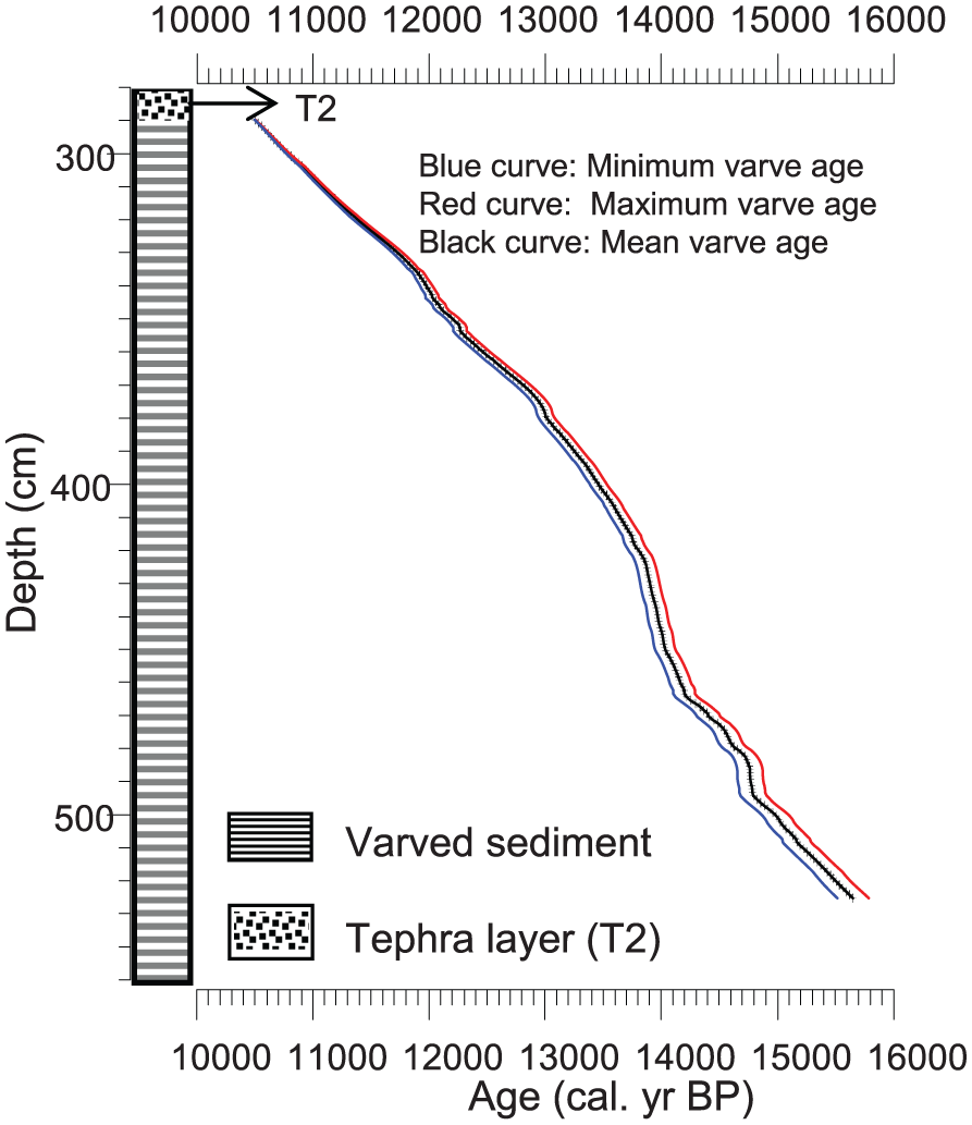
Varve ages versus sediment core depth.

A total of two types of varve (clastic varves and clastic-organic varves) are observed in the sediments (Figure 3). A clastic-organic varve consists of a light minerogenic layer and a dark organic lamina (Figure 3a). The dark organic lamina is mainly composed of diatoms, chrysophyte cysts, and organic material under polarized light. Clastic varves are composed of a coarse silt layer and a fine clay lamina (Figure 3b and c). Varve thicknesses vary from 0.1 to 12 mm, with a mean value of 0.77 mm. Some clastic varves are very thick with thickness ranging from 1 up to 12 mm (Figure 3c). These thick varves are composed of well-sorted subannual layer clastic layers (Figure 3c).

Figure 3.

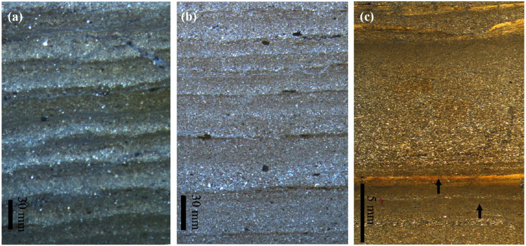
Photomicrographs of clastic-organic and clastic varves: (a) early Holocene clastic-organic varves viewed under a stereoscopic microscope (partly polarized light), (b) clastic varves viewed under a stereoscopic microscope (partly polarized light), and (c) thick clastic varves viewed under a stereoscopic microscope (partly polarized light).

Figure 2 shows the three varve counts used to establish the varve chronology. Maximum varve age (red line), minimum varve age (blue line), and mean varve age (black line) are shown in Figure 2, respectively. In this study, we use the ages derived from the mean varve count (Figure 2). Varve chronological errors do exist due to the presence of subannual layers or less distinct couplets of some varves. The varve chronology error is about 5% as estimated by recounting the varves three times.

Alkenone distribution

Most of the analyzed samples during the last deglaciation contained sufficient amounts of LCKs to be measured by GC. The concentrations of C₃₇ and C₃₈ alkenones exhibit a large range of variation from 0.42 to 28.47 µg/g (dry weight) with a mean of 6.35 µg/g (Figure 4b). Most samples from the BA (14.7–12.85 ka BP) and the YD (12.85–11.5 ka BP) have higher concentrations of LCKs. The higher LCK concentration may be due to biotic interactions among the different algal groups and interplay between climate effects and lake internal forcing.

Figure 4.

Profile of varve thickness and long-chain alkenone (LCK) proxies in the sediments of Lake Sihailongwan: (a) varve thickness (mean value per centimeter), (b) LCK concentrations of C₃₇ and C₃₈ alkenones, (c) C_37:4 %, (d) C₃₇/C₃₈ ratio (a C₃₈ concentration of zero is indicated by 20), and (e) alkenone-derived water temperature during the growing season.

There is a relatively high abundance of the tetra-unsaturated compound (C_37:4) in the sediments, varying between 20% and 60%, except for two values which are above this range (Figure 4c; Supplementary Table S1, available online). All the analyzed samples exhibit a decrease in concentration with increasing chain length (C₃₇ > C₃₈). C₃₇/C₃₈ ratios in most of the samples vary within a narrow range (0.5–2.0%), with only eight samples out of the range. A total of two samples have no C₃₈ alkenones (indicated by value of 20 in the C₃₇/C₃₈; Figure 4d; Supplementary Table S1, available online).

Temperature reconstruction

In the maar lake Sihailongwan, alkenone-based temperature has been interpreted as water temperature during the ‘growing season’ (Chu et al., 2012). In this study, alkenone-derived temperatures were also calculated using a formula derived from a batch culture experiment (Sun et al., 2007):

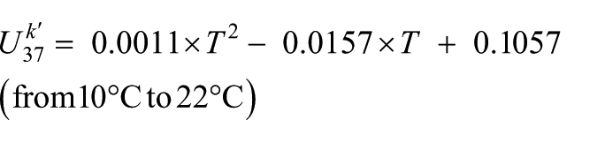
U_{37}^{k^{'}} = 0.0011 \times T^{2} - 0.0157 \times T + 0.1057 (from 10 ° C to 22 ° C)

Figure 4e shows a time series of alkenone-derived water temperature during the growing season (T_w) at Lake Sihailongwan spanning the interval from 15.40 to 10.90 ka BP (Figure 4e). A few data points exceed the lower limit of the culture calibration curve (below 10°C; Sun et al., 2007). It has been noted that the $U_{37}^{k^{'}}$ temperature calibration was nonlinear at relatively low and relatively high temperatures, which probably indicates that the temperature adaptation of cells is limited by the extremes of their growing temperature range (e.g. Conte et al., 1998). Given this uncertainty, we exclude data values below 10°C from subsequent discussions.

In the OD (15.40–14.70 ka BP), the average water temperature was about 11.8°C (excluding data below 10°C). The temperature increased abruptly from 11.0°C at 14.76 ka BP to a peak value of 17.1°C at 14.54 ka BP. In the BA (14.7–12.9 ka BP), the mean water temperature during the growing season was about 15.7°C. A total of two significant cold intervals occurred during the Older Dryas (14.3–14.0 ka BP) and the intra-Allerød cold period (IACP; 13.4–13.1 ka BP). The onset of the YD was relatively gradual, with a slight decrease of 1.5°C from 13.0 to 12.9 ka BP. The average temperature during the YD (12.9–11.5 ka BP) was 14.2°C, which was about 2.4°C warmer than during the OD (11.8°C). The end of the YD shows a rapid temperature increase from 12.5°C at 11.5 ka BP to 17°C at 11.4 ka BP (Figure 5), and large fluctuations (ranging from 13.5°C to 20°C; mean = 15.9°C) are observed during the early Holocene.

Figure 5.

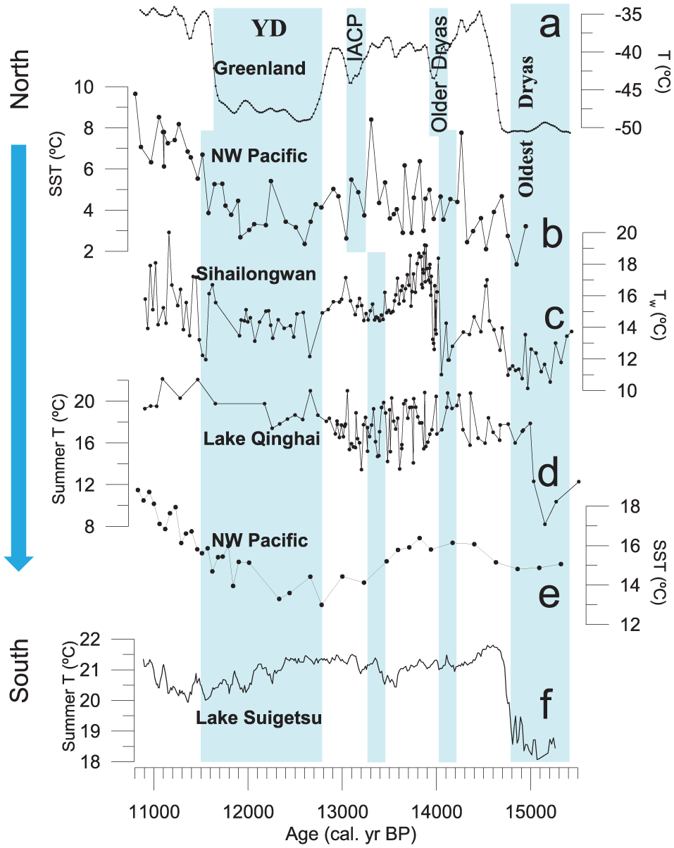
Comparison of the alkenone-inferred paleotemperature record with paleotemperature records from Greenland and the adjacent region: (a) Greenland δ¹⁵N-based temperature reconstruction (average of NEEM, GISP2, and NGRIP; Buizert et al., 2014), (b) alkenone-based sea surface temperature (SST) record from core SO201-2-12KL (Max et al., 2012), (c) alkenone-inferred water temperature for the growing season in Lake Sihailongwan (data below 10°C are excluded), (d) alkenone-based summer temperature record from Lake Qinghai (Hou et al., 2016), (e) alkenone-based SST record from core MD01-2421 (Isono et al., 2009), and (f) pollen-based summer temperature record (5-point running average) from Lake Suigetsu (Nakagawa et al., 2003). A 250-year correction has been applied to adjust the chronology (Shen et al., 2010).

Discussion

Varve chronology

Previous independent radiometric dating results (¹³⁷Cs, ²¹⁰Pb, and AMS ¹⁴C) and monthly sediment trap data have demonstrated the annual nature of sedimentary laminations (Chu et al., 2005; Mingram et al., 2004; Schettler et al., 2006). In Lake Sihailongwan, diatomaceous varves are dominant in the Holocene, while clastic varves and clastic-organic varves are most common in the last deglaciation.

Generally, clastic varves predominate under cold climatic conditions such as in polar and alpine regions due to the lower sedimentary organic matter content and intensive physical weathering that results in large quantities of minerogenic matter being transported into lakes (Francus et al., 2008; Lamoureux, 2001; Ojala et al., 2013; Zolitschka et al., 2015). In Lake Sihailongwan, coarser clastic particles are deposited rapidly either directly from melting lake ice or from surface runoff derived from snowmelt in early spring (Zhu et al., 2013). The fine silt–clay layer may be formed during winter when suspended clay is deposited in a still water environment under ice-cover conditions (Figure 3b). Some clastic varves are very thick, and it was suggested that coarser clastic particles (graded event layers) may indicate enhanced surface runoff, probably caused by reappearance of permafrost and/or reduced vegetation cover and resulting unstable soils (Stebich et al., 2009; Figure 3c).

The appearance of these thick varves resembles ‘glacial varves’ reported in the Arctic and other glaciated areas that are composed of a thick light layer and a thin dark layer (clay cap; Francus et al., 2008; Lamoureux, 2001). In some cases, two or more subannual laminae can be observed in one varve year (Figure 3c). In periglacial lakes, these subannual laminae may result from high discharge into lakes (from rapid snowmelt or flood events). In Lake Sihailongwan, which is a small closed lake, these varves are probably related to the thawing of permafrost.

Uncertainties in alkenone-derived temperature reconstruction

Different temperature calibrations have been reported for lakes (e.g. Chu et al., 2005; D’Andrea et al., 2016; Pearson et al., 2008; Sun et al., 2007; Toney et al., 2010; Wang et al., 2015; Zink et al., 2001). One of the problems for lake calibration is strong seasonal difference due to seasonal variations in precursor organism productivity, which impacts a bias to the reconstructed time series, especially in extra tropical regions (Chu et al., 2012; D’Andrea et al., 2016; Longo et al., 2016).

In the maar lake Sihailongwan, the ice often has a thick snow cover during winter. This reduces light penetration into the water and limits the growth of alkenone precursor organisms. Thus, alkenone-based temperature should represent the water temperature only during the growing season when the lake is ice-free. The calculated temperature from core-top samples is 20.2°C (Chu et al., 2012). This is close to instrumental water temperature measured for the lake during the summer (May 1 to October 30; mean value = 18.5°C) observed from 2007 to 2012 (Supplementary Figure S2, available online). However, there is a 1.7°C difference between observed and reconstructed temperatures.

In most oceanographic settings, C_37:4 concentration is low in the sediments and some alkenone producers (Emiliania huxleyi and Gephyrocapsa oceanica). Therefore, this uncertainty is not significant. In lacustrine sediment, however, the tetra-unsaturated C₃₇ alkenones (C_37:4) is always a problem for quantitative temperature reconstruction since higher abundance of the tetra-unsaturated compound is a common characteristic in limnic systems. Different opinions about principal controlling factors on C_37:4 concentration have been presented in previous literatures, such as changes in alkenone producer (Chu et al., 2005; Theroux et al., 2010), an indicator of salinity on a regional scale (e.g. Liu et al., 2008), temperature dependence (e.g. Toney et al., 2010), and biogenic factors (alkenone biosynthetic pathways and environmental factors; e.g. Chu et al., 2005; Freeman and Wakeham, 1992).

Based on investigating alkenone distributions in lakes of the Qinghai-Tibetan Plateau, Liu et al. (2008, 2011) found that C_37:4 % values are negatively correlated with salinity. They suggested that the C_37:4 % values may be an indicator of salinity at least on a regional scale, with higher values corresponding to lower salinity (Liu et al., 2006, 2008, 2011). However, culture experiments showed that C_37:4 % values from the lake species C. lamellosa varied from 25% to 6% under constant salinity (Sun et al., 2007). In Lake George, C_37:4 % values in the surface waters varied from 80% to 50% as water temperatures varied from 2°C to 23.5°C (Toney et al., 2010). A culture experiment showed that the percentage of C_37:4 decreased as the bloom period progressed in all samples, suggesting that the Hap-B phylotype became active once the Hap-A phylotype began to decline (Toney et al., 2012). In the maar lake Sihailongwan, sediments have higher abundance of the tetra-unsaturated and show large change in some samples (Figure 4c; Supplementary Table S1, available online). It is unlikely controlled by salinity since it is a fresh water and deep lake, and salinity may not be as variable as the percentage of C_37:4 implicated. In addition to salinity, alkenone biosynthetic pathways and environmental factors (nutrient level and light) could affect the desaturation process of C₃₇ alkenones (Freeman and Wakeham, 1992).

The C₃₇/C₃₈ ratio has been used to estimate different haptophyte species (e.g. Chu et al., 2005; Pearson et al., 2008; Toney et al., 2010; Wang et al., 2015; Warden et al., 2016) that may result in unreliable reconstructed temperature values in lacustrine studies. In general, lower C₃₇/C₃₈ ratios are likely to be related to the presence of species such as E. huxleyi, G. oceanica, and C. lamellosa, while higher C₃₇/C₃₈ values are likely to reflect the presence of I. galbana (Wang et al., 2015). In Lake Sihailongwan, the C₃₇/C₃₈ ratios of most analyzed samples vary in a narrow range that may not significantly affect the calibration. However, species effects may be only one of several possible explanations, and the physiological state of the organisms and changes in salinity may also affect the C₃₇/C₃₈ ratio (Kasper et al., 2015; Wang et al., 2015). This question, however, is still unclear because of poor knowledge about haptophyte species and biosynthetic pathways.

Comparison of regional paleotemperature records

Spatial paleoclimatic variation is useful to valuate and verify the sensitivities of different temperature proxy records. We compare the alkenone-derived temperature during the growing season in this study with the δ¹⁵N-based temperature reconstruction from Greenland ice cores (Buizert et al., 2014) and selected quantitative temperature records from adjacent regions (Figure 5). In Lake Sihailongwan, the average water temperature during the YD was about 2.2°C warmer than during the OD (Figure 5b). This is in agreement with the δ¹⁵N-based temperature reconstruction (the YD was 4.5°C warmer than the OD) from Greenland ice cores (Buizert et al., 2014) but contrasts with the δ¹⁸O-based time series (the YD was 4–5°C colder than the OD). It highlights the importance of carbon dioxide forcing and summer insolation in the course of the last deglaciation since the Atlantic meridional overturning circulation (AMOC) strength during the OD was the same or weaker than in the YD (e.g. Buizert et al., 2014). Although a roughly similar pattern of variations can be observed between the alkenone-derived and the δ¹⁵N-based time series, there are several notable differences.

First, there is an ~200-year difference between the two time series for the YD. This may be caused by uncertainties in varve chronology, such as the presence of subannual layers in clastic varves and poor-resolved lamination except the uncertainty at the anchored point. Second, the alkenone-inferred temperature during the YD decreased by only 2–4°C, which is much less than observed in Greenland ice cores (Alley, 2000; Buizert et al., 2014). This could be explained by temperature records from Greenland ice cores being highly weighted toward the winter season (Buizert et al., 2014; Denton et al., 2005), while the alkenone-based temperature reconstruction is biased toward summer (Hou et al., 2016; Isono et al., 2009; Max et al., 2012; Nakagawa et al., 2003; Figure 5).

Finally, a pronounced cold interval is evident for the Older Dryas (14.3–14.0 ka BP; Figure 5c), which is accompanied by an increase in the abundance of herb pollen (mainly Artemisia, Cyperaceae, Poaceae, and Thalictrum) in the Sihailongwan pollen record (Stebich et al., 2009). However, only a few records reveal such a pronounced cold interval, such as the chironomid-inferred July air temperature record from Ech paleolake (Millet et al., 2012) and a hydrologic δD_wax record from a sediment core from the Gulf of Aden (Tierney and DeMenocal, 2013). More high-resolution temperature records are needed to confirm whether this cold interval is a consistent feature of the Asian monsoon region.

Although a roughly similar variation can be observed in quantitative temperature records from adjacent regions, there are significant differences among regional paleotemperature records derived from the Asian monsoon region (Figure 5). These discrepancies may be partly due to genuine spatial differences in climate as well as to uncertainties in proxy interpretation and dating. For example, a 200- to 500-year correction has been applied to adjust the chronology of the pollen-based summer temperature record from Lake Suigetsu (e.g. Shen et al., 2010). More research is needed to verify the occurrence of regional climatic variability and the uncertainties of different proxies.

Comparison with monsoon proxy records

In the Asian monsoon region, well-dated stalagmite δ¹⁸O records reveal distinct paleoclimatic changes, such as the OD, BA, and YD, although there is an ongoing debate as to whether stable oxygen isotope ratios primarily reflect variations in the amount of precipitation, monsoon strength, inter-hemispheric temperature gradients, or air mass source (e.g. Maher and Thompson, 2012). Within the limits of dating uncertainties, the changes in alkenone-based water temperature exhibit a pattern resembling that of stalagmite monsoon proxy records at millennial timescales (Figure 6). In general, the colder summer intervals recorded in Lake Sihailongwan were generally associated with heavier stalagmite δ¹⁸O values (weaker summer monsoon), both in southeastern China (Wang et al., 2001) and northeastern Asia (Ma et al., 2012; Shen et al., 2010; Figure 6). This supports that colder summer temperature on land may reduce the land–sea thermal contrast and weakens the Asian summer monsoon.

Figure 6.

Comparison of alkenone-derived paleotemperature and monsoon proxy records: (a) stalagmite δ¹⁸O records from Kulishu Cave (Ma et al., 2012) and Maboroshi Cave (blue line; Shen et al., 2010) in northeastern Asia, (b) alkenone-inferred water temperature during the growing season (this study), (c) record of herb pollen percentages in Lake Sihailongwan (Stebich et al., 2009), and (d) stalagmite δ¹⁸O record from Hulu Cave in southeastern China (Wang et al., 2001). The δ¹⁸O data between 10,800 and 14,940 cal. yr BP are from stalagmite sample PD; those between 14,940 and 15,500 cal. yr BP are from stalagmite sample YT (Wang et al., 2001).

On decadal to centennial timescales, however, there are noticeable discrepancies in the stalagmite δ¹⁸O records and the temperature record from Lake Sihailongwan due to uncertainties in dating. Additionally, the discrepancies could be caused by variations in the EASM being closely related to several atmospheric–oceanic processes (e.g. El Niño–Southern Oscillation, Pacific Decadal Oscillation, and Arctic Oscillation) which evolve at different spatial and temporal scales (Cobb et al., 2003; Wang et al., 2014).

Conclusion

In the maar lake Sihailongwan, alkenone-based temperature is interpreted as reflecting water temperature during the growing season when the lake is ice-free. Variations in alkenone-based temperature reveal a distinctive pattern during the last deglaciation: a temperature increase of 6°C at the onset of the BA, two cold intervals (during the Older Dryas and the IACP), a relatively minor temperature decrease of 1–3°C during the YD, and a rapid temperature increase of 4–5°C at the early Holocene.

The YD was about 2.2°C warmer than the OD, which highlights the importance of carbon dioxide forcing and summer insolation as previously suggested (e.g. Buizert et al., 2014). The alkenone-based ‘summer’ temperature changes observed in Lake Sihailongwan were minor than coeval records from Greenland ice cores that are weighted toward winter conditions. It may support an early hypothesis that abrupt climate change is mostly a winter phenomenon.

Within the limits of dating uncertainties, the changes in alkenone-based temperature exhibit a pattern resembling that of the stalagmite monsoon proxy records at millennial timescales. In general, the colder summer intervals recorded in Lake Sihailongwan were associated with heavier stalagmite δ¹⁸O values (weaker summer monsoon). This supports that colder summer temperature on land may reduce the land–sea thermal contrast and weakens the Asian summer monsoon.

Supplemental Material

Supplementary_Material – Supplemental material for Long-chain alkenone-inferred temperatures from the last deglaciation to the early Holocene recorded by annually laminated sediments of the maar lake Sihailongwan, northeastern China

Supplemental material, Supplementary_Material for Long-chain alkenone-inferred temperatures from the last deglaciation to the early Holocene recorded by annually laminated sediments of the maar lake Sihailongwan, northeastern China by Qing Sun, Guoqiang Chu, Manman Xie, Yuan Ling, Youliang Su, Qingzeng Zhu, Yabin Shan and Jiaqi Liu in The Holocene

Footnotes

Acknowledgements

We would like to thank two anonymous reviewers for constructive comments and correcting the English.

Funding

This research was jointly supported by the National Natural Science Foundation of China (grant nos 41272198, 41371219, and 41672174) and the Science Research Found of the Chinese Academy of Geological Science (grant no. YYWF201618).

ORCID iD

Qing Sun

References

Alley

(2000) The Younger Dryas cold interval as viewed from central Greenland. Quaternary Science Review 19: 213–226.

Buizert

Gkinis

Severinghaus

et al . (2014) Greenland temperature response to climate forcing during the last deglaciation. Science 345: 1177–1180.

Chu

Sun

Wang

et al . (2012) Seasonal temperature variability during the past 1600 years recorded in historical documents and varved lake sediment profiles from northeastern China. The Holocene 22: 785–792.

Chu

Sun

Zheng

et al . (2005) Long-chain alkenone distributions and temperature dependence in lacustrine surface sediments from China. Geochimica et Cosmochimica Acta 69: 4985–5003.

Cobb

Charles

Cheng

et al . (2003) El Niño/Southern Oscillation and tropical Pacific climate during the last millennium. Nature 424: 271–276.

Conte

Thompson

Lesley

et al . (1998) Genetic and physiological influences on the alkenone/alkenoate versus growth temperature relationship in Emiliania huxleyi and Gephyrocapsa oceanica. Geochimica et Cosmochimica Acta 62: 51–68.

D’Andrea

Theroux

Bradley

et al . (2016) Does phylogeny control

U_{37}^{k^{'}}

temperature sensitivity? Implications for lacustrine alkenone paleothermometry. Geochimica et Cosmochimica Acta 175: 168–180.

Denton

Alley

Comer

et al . (2005). The role of seasonality in abrupt climate change. Quaternary Science Reviews 24: 1159–1182.

Francus

Bradley

Lewis

et al . (2008) Limnological and sedimentary processes at Sawtooth Lake, Canadian High Arctic, and their influence on varve formation. Journal of Paleolimnology 40: 963–985.

10.

Freeman

Wakeham

(1992) Variations in the distributions and isotopic compositions of alkenones in Black Sea particles and sediments. Organic Geochemistry 19: 277–285.

11.

Hou

Huang

Zhao

et al . (2016) Large Holocene summer temperature oscillations and impact on the peopling of the northeastern Tibetan Plateau. Geophysical Research Letters 43: 1323–1330.

12.

Isono

Yamamoto

Irino

et al . (2009) The 1500-year climate oscillation in the midlatitude North Pacific during the Holocene. Geology 37: 591–594.

13.

Kasper

van der Meer

MTJ

Castañeda

et al . (2015) Testing the alkenone D/H ratio as a paleo indicator of sea surface salinity in a coastal ocean margin (Mozambique Channel). Organic Geochemistry 78: 62–68.

14.

Lamoureux

(2001) Varve chronology techniques. In: Last

Smol

(eds) Developments in Paleoenvironmental Research (DPER), Tracking Environmental Change Using Lake Sediments: Basin Analysis, Coring, and Chronological Techniques, vol. 1. Dordrecht: Kluwer, pp. 247–260.

15.

Battisti

Schrag

et al . (2005) Abrupt climate shifts in Greenland due to displacements of the sea ice edge. Geophysical Research Letters 32: L19702.

16.

Liang

Hou

et al . (2015) Centennial-scale climate variability during the past 2000 years on the central Tibetan Plateau. The Holocene 25: 892–899.

17.

Liu

et al . (2008) Distribution of the C37 tetra-unsaturated alkenone in Lake Qinghai, China: A potential lake salinity indicator. Geochimica et Cosmochimica Acta 72: 988–997.

18.

Liu

Wang

et al . (2011) Salinity control on long-chain alkenone distributions in lake surface waters and sediments of the northern Qinghai-Tibetan Plateau, China. Geochimica et Cosmochimica Acta 75: 1693–1703.

19.

Liu

Henderson

ACG

Huang

(2006) Alkenone-based reconstruction of late-Holocene surface temperature and salinity changes in Lake Qinghai, China. Geophysical Research Letters 33: L09707.

20.

Longo

Theroux

Giblin

et al . (2016). Temperature calibration and phylogenetically distinct distributions for freshwater alkenones: Evidence from northern Alaskan lakes. Geochimica et Cosmochimica Acta 180: 177–196.

21.

Cheng

Tan

et al . (2012) Timing and structure of the Younger Dryas event in northern China. Quaternary Science Reviews 41: 83–93.

22.

Maher

Thompson

(2012) Oxygen isotopes from Chinese caves: Records not of monsoon rainfall but of circulation regime. Journal of Quaternary Science 27: 615–624.

23.

Max

Riethdorf

Tiedemann

et al . (2012) Sea surface temperature variability and sea-ice extent in the subarctic northwest Pacific during the past 15,000 years. Paleoceanography 27: PA3213.

24.

Millet

Rius

Galop

et al . (2012) Chironomid-based reconstruction of Lateglacial summer temperatures from the Ech palaeolake record (French western Pyrenees). Palaeogeography, Palaeoclimatology, Palaeoecology 315–316: 86–99.

25.

Mingram

Allen

JRM

Brüchmann

et al . (2004) Maar- and crater lakes of the Long Gang Volcanic Field (N.E. China) – Overview, laminated sediments, and vegetation history of the last 900 years. Quaternary International 123–125: 135–147.

26.

Nakagawa

Kitagawa

Yasuda

et al . (2003) Asynchronous climate changes in the North Atlantic and Japan during the last termination. Science 299: 688–691.

27.

Nakamura

Sawada

Araie

et al . (2016) Composition of long chain alkenones and alkenoates as a function of growth temperature in marine haptophyte Tisochrysis lutea. Organic Geochemistry 99: 78–89.

28.

Ojala

AEK

Kosonen

Weckström

et al . (2013) Seasonal formation of clastic-biogenic varves: The potential for palaeoenvironmental interpretations. GFF 135: 237–247.

29.

Parplies

Lücke

Vos

et al . (2008) Late glacial environment and climate development in northeastern China derived from geochemical and isotopic investigations of the varved sediment record from Lake Sihailongwan (Jilin Province). Journal of Paleolimnology 40: 471–487.

30.

Pearson

Juggins

Farrimond

(2008) Distribution and significance of long-chain alkenones as salinity and temperature indicators in Spanish saline lake sediments. Geochimica et Cosmochimica Acta 72: 4035–4046.

31.

Schettler

Mingram

Liu

et al . (2006) East-Asian monsoon variability between 15,000 and 2000 cal. yr BP recorded in varved sediments of Lake Sihailongwan (northeastern China, Long Gang volcanic field). The Holocene 16: 1043–1057.

32.

Shen

Kano

Hori

et al . (2010) East Asian monsoon evolution and reconciliation of climate records from Japan and Greenland during the last deglaciation. Quaternary Science Reviews 29: 3327–3335.

33.

Song

Zhou

Zhang

et al . (2015) Solar imprints on Asian inland moisture fluctuations over the last millennium. The Holocene 25: 11935–11943.

34.

Stebich

Mingram

Han

et al . (2009) Late Pleistocene spread of (cool-) temperate forests in northeast China and climate changes synchronous with the North Atlantic region. Global and Planetary Change 65: 56–70.

35.

Stebich

Rehfeld

Schlütz

et al . (2015) Holocene vegetation and climate dynamics of NE China based on the pollen record from Sihailongwan Maar Lake. Quaternary Science Reviews 124: 275–289.

36.

Sun

Chu

Liu

et al . (2007) Calibration of alkenone unsaturation index with growth temperature for a lacustrine species, Chrysotila lamellosa (Haptophyceae). Organic Geochemistry 38: 1226–1234.

37.

Theissen

Zinniker

Moldowan

et al . (2005) Pronounced occurrence of long-chain alkenones and dinosterol in a 25,000-year lipid molecular fossil record from Lake Titicaca, South America. Geochimica et Cosmochimica Acta 69: 623–636.

38.

Theroux

D’Andrea

Toney

et al . (2010). Phylogenetic diversity and evolutionary relatedness of alkenone-producing haptophyte algae in lakes: Implications for continental paleotemperature reconstructions. Earth Planetary and Science Letters 300: 311–320.

39.

Theroux

Toney

Amaral-Zettler

et al . (2013) Production and temperature sensitivity of long chain alkenones in the cultured haptophyte Pseudoisochrysis paradoxa. Organic Geochemistry 62: 68–73.

40.

Tierney

DeMenocal

(2013). Abrupt shifts in Horn of Africa hydroclimate since the last glacial maximum. Science 342: 843–846.

41.

Toney

Huang

Fritz

et al . (2010) Climatic and environmental controls on the occurrence and distributions of long chain alkenones in lakes of the interior United States. Geochimica et Cosmochimica Acta 74: 1563–1578.

42.

Toney

Theroux

Andersen

et al . (2012) Culturing of the first 37:4 predominant lacustrine haptophyte: Geochemical, biochemical, and genetic implications. Geochimica et Cosmochimica Acta 78: 51–64.

43.

Wang

Cheng

et al . (2014) The global monsoon across timescales: Coherent variability of regional monsoons. Climate of the Past 10: 2007–2052.

44.

Wang

Cheng

Edwards

et al . (2001) A high-resolution absolute-dated late Pleistocene monsoon record from Hulu Cave, China. Science 294: 2345–2348.

45.

Wang

Liu

Zhang

et al . (2015) A new approach for reconstructing Holocene temperatures from a multi-species long chain alkenone record from Lake Qinghai on the northeastern Tibetan Plateau. Organic Geochemistry 88: 50–58.

46.

Warden

van der Meer

MTJ

Moros

et al . (2016) Sedimentary alkenone distributions reflect salinity changes in the Baltic Sea over the Holocene. Organic Geochemistry 102: 30–44.

47.

Liu

Wang

et al . (2016) Vegetation and climate change during the last deglaciation in the Great Khingan Mountain, Northeastern China. PLoS ONE 1: e0146261.

48.

Xiao

Haberle

Shen

et al . (2014) Latest pleistocene and Holocene vegetation and climate history inferred from an alpine lacustrine record, northwestern Yunnan Province, southwestern China. Quaternary Science Reviews 86: 35–48.

49.

Zhao

Liu

Rohling

et al . (2013) Holocene temperature fluctuations in the Northern Tibetan Plateau. Quaternary Research 80: 55–65.

50.

Zhu

Mingram

Brauer

(2013) Early Holocene aeolian dust accumulation in northeast China recorded in varved sediments from Lake Sihailongwan. Quaternary International 290–291: 299–312.

51.

Zink

Leythaeuser

Melkonian

et al . (2001) Temperature dependency of long-chain alkenone distributions in recent to fossil limnic sediments and in lake waters. Geochimica et Cosmochimica Acta 65: 253–265.

52.

Zolitschka

Francus

Ojala

AEK

et al . (2015) Varves in lake sediments – A review. Quaternary Science Reviews 117: 1–41.

Supplementary Material

Please find the following supplemental material available below.

For Open Access articles published under a Creative Commons License, all supplemental material carries the same license as the article it is associated with.

For non-Open Access articles published, all supplemental material carries a non-exclusive license, and permission requests for re-use of supplemental material or any part of supplemental material shall be sent directly to the copyright owner as specified in the copyright notice associated with the article.

0.00 MB

0.93 MB