Comparing and improving methods for reconstructing peatland water-table depth from testate amoebae

Abstract

Proxies that use changes in the composition of ecological communities to reconstruct temporal changes in an environmental covariate are commonly used in paleoclimatology and paleolimnology. Existing methods, such as weighted averaging and modern analog technique, relate compositional data to the covariate in very simple ways, and different methods are seldom compared systematically. We present a new Bayesian model that better represents the underlying data and the complexity in the relationships between species’ abundances and a paleoenvironmental covariate. Using testate amoeba–based reconstructions of water-table depth as a test case, we systematically compare new and existing models in a cross-validation experiment on a large training dataset from North America. We then apply the different models to a new 7500-year record of testate amoeba assemblages from Caribou Bog in Maine and compare the resulting water-table depth reconstructions. We find that Bayesian models represent an improvement over existing methods in three key ways: more complete use of the underlying compositional data, full and meaningful treatment of uncertainty, and clear paths toward methodological improvements. Furthermore, we highlight how developing and systematically comparing methods lead to an improved understanding of the proxy system. This paper focuses on testate amoebae and water-table depth, but the framework and ideas are widely applicable to other proxies based on compositional data.

Keywords

Bayesian statistics compositional data Holocene hydrology North America Northeast United States peatlands paleoclimate statistical methods testate amoebae

Introduction

For more than a century, paleoecologists, paleolimnologists, and paleoceanographers have tried to infer environmental changes from temporal changes in the composition of ecological communities preserved in sediments (Edwards et al., 2017). Early work focused on qualitative assessments of the environmental affinities of different species or groups of species (Hustedt, 1939 [1937]; Iversen, 1944; Nygaard, 1956; Phleger, 1953; Von Post, 1918; Wright et al., 1963). By the 1970s, qualitative approaches began to give way to quantitative reconstructions. This shift was led by formative work of John Imbrie and colleagues. In a benchmark paper, Imbrie and Kipp (1971) introduced a framework for quantitative reconstruction of past environments from compositional data using transfer functions (Imbrie et al., 1973; Imbrie and Kipp, 1971). Transfer functions aim to formally and quantitatively relate changes in the composition of an ecological community to changes in a paleoenvironmental covariate.

Imbrie’s work centered on the marine realm, using foraminifera to reconstruct past sea surface temperatures. However, similar techniques were simultaneously being developed for paleoclimatological inference from terrestrial data (e.g. pollen) (Imbrie and Webb, 1981; Webb and Bryson, 1972) and were soon applied to other kinds of paleoecological data. Researchers have successfully used many different types of organisms to infer many different target variables. Some examples include reconstructing temperature and precipitation changes via changes in the surrounding vegetation as recorded by pollen (Webb and Bryson, 1972), inferring bog water-table depth (WTD) histories using changes in testate amoebae assemblages (Warner and Charman, 1994; Woodland et al., 1998), and generating records of lake pH and salinity based on the types of diatoms living in the lakes and preserved in sediment cores (Battarbee et al., 2002).

In particular, diatom-based pH reconstructions were a key testbed for development of quantitative methodologies. Researchers applied many possible methodologies to the problem of how to best reconstruct the pH of lakes based on diatom assemblages preserved in sediments (Battarbee, 1984; Birks et al., 1990; Charles, 1985; Davis et al., 1985; Oehlert, 1988; Renberg et al., 1985). This work led to application of diatom-based pH reconstructions in Europe and the United States as a key line of evidence in determining the effects of acid precipitation on lake systems. Ultimately, these paleolimnological studies were a major factor in environmental policy changes, including the 1990 amendments to the Clean Air Act (Smol, 2009).

Applications of transfer functions have continued to the present, including important work to understand potential pitfalls and improve inferences. Examples include understanding the effects of spatial autocorrelation (Telford and Birks, 2009), differential preservation (Mitchell et al., 2008), and considering appropriate ecological models (Juggins, 2013). Furthermore, there has been important work on cross-validation and uncertainty estimation (Payne et al., 2012; Telford et al., 2004; Trachsel and Telford, 2016). Despite these advances and applications, there has been little fundamental rethinking of the underlying methodologies (Birks and Simpson, 2013): simple models like weighted averaging (WA) are still widely used in paleoenvironmental reconstructions from paleoecological data.

A logical step toward innovation for proxies based on compositional data is to take advantage of state-of-the-art Bayesian statistical techniques. Bayesian methods have started to be applied to compositional data (Salonen et al., 2012; Toivonen et al., 2001), but they have not seen wide use in the community. Bayesian models allow for a more realistic representation of underlying ecological responses to changes in the environment, inference on the underlying ecological processes, and a more formal and thorough treatment of all sources of uncertainty.

Uncertainties are a key part of any proxy reconstruction because they represent our confidence in the inferences being made. Paleoclimate records based on compositional data are important indicators of terrestrial climate over the Holocene (Marlon et al., 2017; Shuman et al., 2018). Thus, when these proxies are used in climatic synthesis and data assimilation efforts such as PAGES2k (Hydro2k, 2017), the Last Millennium Reanalysis (Hakim et al., 2016), and the PaleoEcological Observatory Network (PalEON) (Marlon et al., 2017), meaningful estimation of uncertainties is necessary to combine and weigh the data coming from the many different sources. It is therefore critical to question and improve inference and uncertainty estimation for proxies based on compositional data.

In this paper, we apply Bayesian statistical tools to the problem of reconstructing an environmental covariate from compositional data. We compare Bayesian methods with a range of existing methods in cross-validation and in reconstruction. The framework we use is general and potentially applicable to any proxy based on compositional data, but we focus on testate amoeba–based reconstructions of WTD in ombrotrophic peat bogs.

Testate amoebae are single-celled organisms that live on the surface of bogs and in lakes, wetlands, and so on. The community composition of testate amoebae living on the surface of ombrotrophic bogs is sensitive to changes in the surface wetness of the bog. Our operational measure of surface wetness is WTD. WTD is measured relative to the peat surface, with high values corresponding to deep water tables (dry surface conditions), low values indicating wetter surface conditions, and negative values indicating standing water (Booth, 2008).

Testate amoebae are a prime target for methodological comparison because we have a large training dataset of surface samples from bogs across North America and a new 7500-year long testate amoebae record from Caribou Bog in Maine. First, we introduce those datasets. Then, we review existing methods for developing transfer functions and introduce our new Bayesian model. Next, we apply these models to the training dataset and perform a cross-validation experiment to test their predictive skill. Finally, we use the models to reconstruct WTD and compare the resulting reconstructions. We discuss specific implications of our results for testate amoebae–based WTD reconstructions and general implications for proxies based on compositional data.

Data and methods

Modern surface sample training dataset

Paleoenvironmental reconstruction from compositional data requires a modern training dataset, in which both the community assemblage and the environmental covariate are measured for a number of sites distributed in space. The training dataset should sample the full range of covariate values expected in reconstruction. Developing a training dataset entails measuring the depth to the water table (the environmental covariate) at many sites on many peatlands, collecting surface samples from the locations of the WTD measurements, and, back in the lab, processing the surface sample and counting the testate amoeba assemblage under a microscope.

We used a large modern training dataset of 978 samples from 68 sites in North America (Figure 1). This dataset contains samples from Booth (2002), Booth (2008), Booth and Zygmunt (2005), and Markel et al. (2010). For the 378 samples from the Booth (2008) dataset, the WTDs were measured using the method of PVC tape discoloration (Booth et al., 2005). This technique produces a measurement of average WTD over a season, which can lead to a WTD estimate more directly analogous to the temporal integration of the testate amoeba surface samples, which are collected instantaneously but represent time-averaged death assemblages (Booth, 2008). The WTDs for samples from datasets other than Booth (2008) were measured instantaneously at the time of collection. For 27 samples, the true WTD was not measured because it was greater than 50 cm below the surface of the bog. These samples were not used because the transfer function methods are not statistically robust to this type of censoring, and in particular, the censored observations affect the convergence of the Bayesian statistical models as formulated in this paper. We note that the elimination of these dry samples may have resulted in a loss of ecological information for some taxa, such as Hyalosphenia subflava. Our training dataset, then, consists of 951 samples. 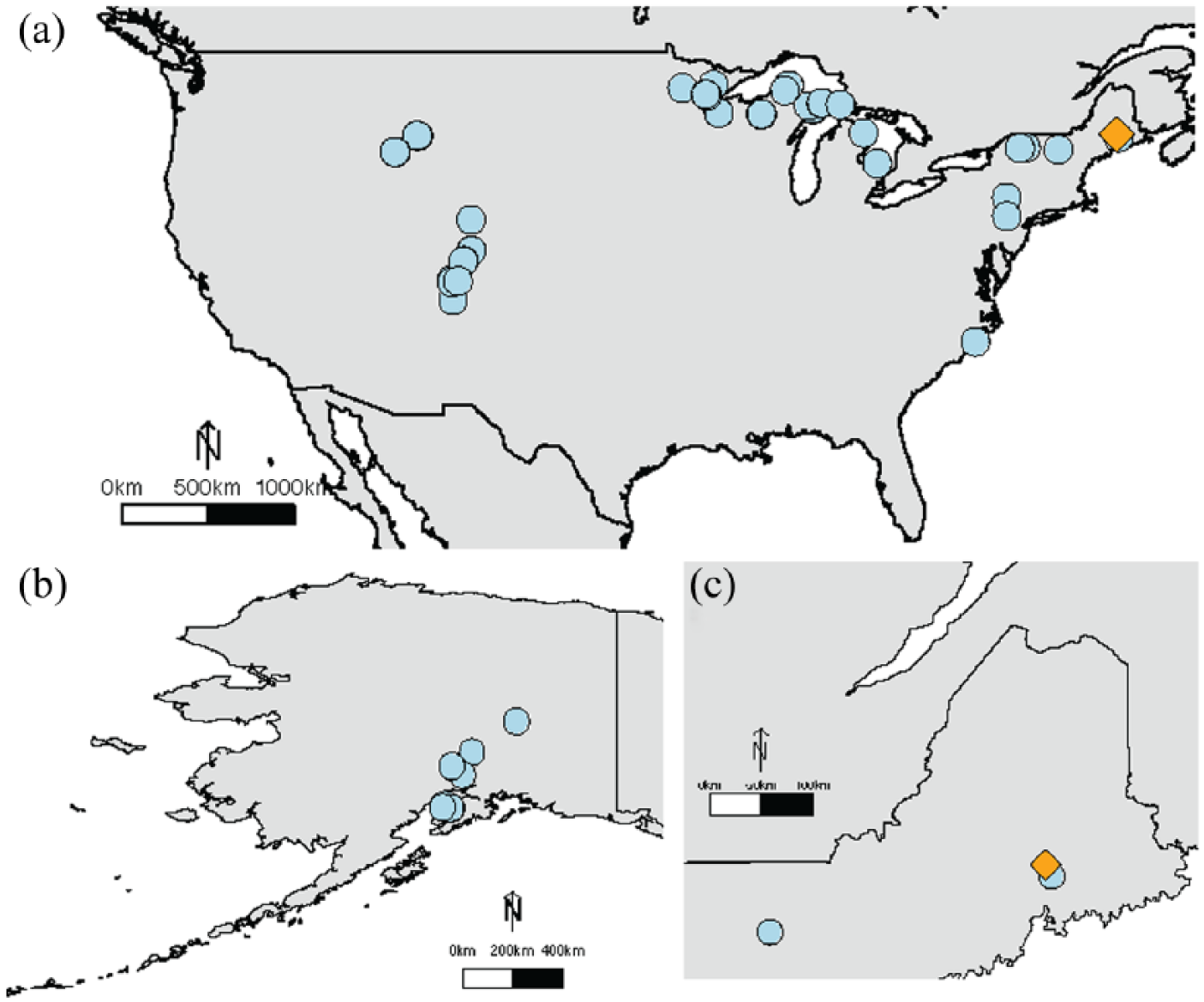In practice, this looks like a vector, $Y$ , of 951 measured WTDs and a matrix, $X$ , where each of the 951 lines corresponds to the observed testate amoeba assemblage from each site. Each column of the matrix $X$ corresponds to a different testate amoebae species.

Figure 1.

Map showing the sites that make up the modern training dataset sites (blue circles) and the site of the new water-table depth reconstruction, Caribou Bog (orange diamond): Panel (a) shows the Continental United States, Panel (b) shows the training dataset sites in Alaska, and Panel (c) zooms in on Maine and the surrounding area.

Site description and lab methods: Reconstruction dataset

Caribou Bog (44.985°N, 68.814°W; elevation: 39 m) is a raised, ombrotrophic peat bog system located in south-central Maine, USA. The bog system (Caribou Bog, Mud Pond, Pushaw Stream wetlands) lies in a series of north-northwest to south-southeast trending features and covers approximately 2400 ha.

The post-glacial development of the peatland has been chronicled by Gajewski (1987) and Hu and Davis (1995). Briefly, after the Laurentide ice sheet receded, the isostatically depressed site was flooded by ocean water. Approximately 14,800 years before present, as the land surface emerged from the sea, an unproductive glacial lake formed. Eventually, organic sediment deposition began, with the oldest organic sediments found by Hu and Davis (1995) dating to approximately 12,300 cal. yr BP. A peatland began to form via terrestrialization around 11,000 yr BP. This began first as a limnic sedge fen before transitioning to an ombrotrophic wooded fen (8300–9000 cal. yr BP), and finally a Sphagnum-dominated peatland (~6400 cal. yr BP) (Hu and Davis, 1995). The site has remained a Sphagnum-dominated ombrotrophic peatland to the present. The dates of the transitions varied in different parts of the bog (Hu and Davis, 1995), and our core suggests that the site was Sphagnum-dominated as far back as 7500 cal. yr BP, but the above provides a general trajectory.

The modern vegetation at the site is an open Sphagnum–Ericaceae peatland with scattered, isolated Picea. There is a narrow Alnus swamp around the edge of the bog (Gajewski, 1987). The surrounding forests contain secondary Betula papyrifera, Abies, and Populus. Prior to European settlement, Tsuga canadensis and Pinus were common in the area (Gajewski, 1987).

Sediment cores were collected in the summer of 2014. We used a 4-in diameter modified piston corer (Wright et al., 1984) to collect the top 251 cm in three drives. We then used a Russian (Jowsey) peat corer to collect 96 cm further in two drives for a total of 347 cm. In the lab, the cores were cut into contiguous 1 cm sections and subsampled for testate amoebae and radiocarbon analyses.

We obtained a 1-cm³ subsample from each 1 cm section of the core for analysis of testate amoebae and pollen and prepared them using standard techniques based on Booth (2010). Samples were boiled in water, sieved to retain the fraction between 15 and 250 μm, dyed with Safranin O, cleaned via two rounds of centrifugation, and stored in glycerol. Testate amoebae were identified and counted at 400× optical magnification to a count of at least 100 individuals per sample.

We obtained 24 radiocarbon dates on Sphagnum stems to develop a chronology for the core (Table S1, available online). Using these dates and the year of collection, we developed an age–depth model with Bchron (Parnell, 2014) (Figure S1, available online). The basal age is approximately 7500 cal. yr BP. The age model and core lithology show no signs of depositional hiatuses. Sedimentation times range from 5 to 30 yr/cm with a median of 18 yr/cm. These are consistent with the regional priors established by Goring et al. (2012).

Models

Basic problem

There are a variety of methods to estimate environmental covariates from compositional data. Some of these tools have ties to formal statistics; others have developed through domain experts’ intuition (Birks, 1998; Juggins and Birks, 2012). Regardless of the complexity or connection to formal statistics, the most widely used methods are underlain by similar general assumptions (Imbrie and Webb, 1981; Juggins, 2013).

The basic idea, following Imbrie and Webb (1981), is that the ecological community assemblage $Y$ is related to the value of some environmental covariate $X$ via an ecological response function $R_{e}$ , such that

Y = R_{e} (X)

In general, we are interested in the inverse prediction problem where we know the ecological assemblage and want to predict the covariate

X = ϕ (Y)

where $ϕ (Y)$ is a so-called transfer function. Having set up this basic problem, we introduce the models that have been used to predict $Y$ based on X. First, we discuss WA, weighted averaging partial least squares (WAPLS), and maximum likelihood response curves (MLRC). These models treat the response of each species to the covariate independently. Then, we introduce two methods that approach the problem differently: modern analog technique (MAT) and random forest (RF). These models use the full assemblage simultaneously to estimate the covariate. Next, we discuss uncertainty estimation for WA, WAPLS, MLRC, MAT, and RF. Finally, we introduce the Bayesian models (BUMMER and MVGP) which are logical extensions and formalizations of the first set of models. The Bayesian approaches model the ecological response of individual species, but in the Bayesian models the responses are modeled jointly to respect the sum-to-N nature of the data.

WA, WAPLS, and MLRC

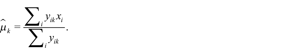
These three transfer function methods are based on the idea that the ecological response of each species to a covariate can be summarized by an optimum value at which the species is most abundant (Gauch and Whittaker, 1972). WA is a very simple procedure that can be written in two equations. First, from the modern training dataset, the estimated optimum ${\hat{μ}}_{k}$ for each of the $k$ observed species is calculated by

{\hat{μ}}_{k} = \frac{\sum_{i} y_{i k} x_{i}}{\sum_{i} y_{i k}} .

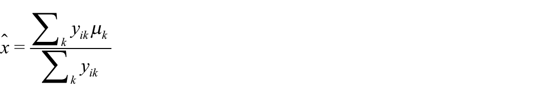
Then, these estimated optima, ${\hat{μ}}_{k}$ , are used to estimate the unobserved covariate $x$ based on the observed assemblage $y$ as follows:

\hat{x} = \frac{\sum_{k} y_{i k} μ_{k}}{\sum_{k} y_{i k}}

The range of WA-inferred covariate at this point is greatly reduced ( ‘shrunk’) compared with the observed range in the training dataset. To correct for this, a linear regression is used to ‘deshrink’ the predictions (Birks et al., 1990; ter Braak and Van Dam, 1989). This can be done in two ways: the so-called ‘classical’ deshrinking regresses the inferred covariate values onto the observed covariate values from the training set, whereas the ‘inverse’ deshrinking regresses the observed values onto the inferred values. Classical deshrinking produces a larger range of ‘deshrunk’ values. Recent work has suggested using a smooth, monotonic spline regression instead of the standard linear regression. (Birks and Simpson, 2013). We suggest that deshrinking to improve the raw WA predictions using a simple regression can be thought of as ‘boosting’ in the language of machine learning. Boosting is defined as using a set of ‘weak learners’ to produce a ‘strong learner’ (Schapire, 1990). The raw WA predictions and the linear regression on their own are weak models; combined together they produce a stronger model.

Despite the simplicity of WA, it has continued to be successful, with wide applications in paleoclimate inference (e.g. Amesbury et al., 2016; Birks and Simpson, 2013; Clifford and Booth, 2013). Some modifications to WA have been proposed, including emphasizing species with narrow tolerances by weighting each species by the inverse of their tolerances (ter Braak and Van Dam, 1989), but in practice this generally has little effect (Juggins and Birks, 2012). Another recent suggested modification was to perform WA on traits instead of species (Van Bellen et al., 2017). The trait-based transfer function performed similarly to standard WA on species.

A modification of WA that can significantly improve predictions in some cases is WAPLS (ter Braak and Juggins, 1993). As the name suggests, WAPLS combines the WA method described above with partial least squares, a dimension-reduction algorithm comparable to principal component analysis. WAPLS with a single PLS component is equivalent to standard WA. Each additional WAPLS component can be thought of as performing WA on the residuals of WA to improve the estimation of the optima. For details of the algorithm, the reader is referred to ter Braak and Juggins (1993) and Juggins and Birks (2012). We suggest that, similar to the deshrinking, WAPLS is another example of boosting (Schapire, 1990). In this case, the weak-learner WA is being applied multiple times to produce a stronger learner.

WA can be thought of as a simplification of MLRC (Birks et al., 1990; Oksanen et al., 1990; ter Braak and Van Dam, 1989). Instead of summarizing a species’ response to the covariate with a simple optima (as in WA), MLRC fits a Gaussian response curve for each species, in turn. Then, in prediction, the curves are used in a maximum likelihood framework to estimate the environmental covariate for an observed assemblage. MLRC is not widely used because the curves are difficult to fit within the maximum likelihood framework and the model often does not perform as well as WA or WAPLS (Juggins and Birks, 2012).

MAT and RF

Whereas WA, WAPLS, and MLRC use the response of each individual species to predict the covariate, a different approach, MAT, uses the full assemblage at once to estimate the covariate (Jackson and Williams, 2004). MAT uses the same training dataset, but instead of estimating a species-by-species response to the covariate, MAT assumes that similar assemblages should be associated with similar covariate values. To estimate the covariate for a given assemblage, MAT finds the k-closest analog assemblages in the training dataset based on a multidimensional distance metric. There are many possible choices for distance metrics, each with unique strengths and weaknesses (Prentice, 1980), but chord distance has become widely used for compositional data (Overpeck et al., 1985). The analog assemblages identified in the training set are each associated with a value of the covariate. For the assemblage of interest, the covariate is estimated by taking the mean (could use median or some weighted mean as well) of the covariates of the analog assemblages. In statistics, MAT is known as k-nearest neighbors. MAT has not been widely applied to testate amoebae, but it is commonly used in the reconstruction of paleoclimate from pollen and other compositional data.

Another analytical approach we apply to the data is RF (Breiman, 2001). RF is a common machine learning technique. Like MAT, RF generates predictions by identifying analogs, but RF uses a very different algorithm. Instead of using a simple multivariate distance metric, RF creates a large number of dichotomous decision trees to identify analogs. RF begins by creating bootstrapped versions of the modern training dataset: the modern training dataset is randomly sampled with replacement to create a bootstrapped training set of the same size as the real training dataset. Then, for each bootstrapped training dataset, RF begins a dichotomous decision tree by choosing a random subset of species and identifying which of those species best splits the observed covariate. This process is repeated at each node until a full decision tree is grown. RF stops when each terminal node satisfies a ‘stop’ condition by containing only a small number of observations or not being able to make a meaningful further split. Many different trees are created to make a ‘random forest’. Then, to make a prediction, an assemblage is run through all of the decision trees. The predicted value of the covariate is the average of the covariate value for each of the terminal nodes identified for the sample over all the trees. For details, the reader is referred to Breiman (2001) and Liaw and Wiener (2002).

Uncertainty estimation

WA, MLRC, MAT, and RF do not produce full predictive distributions, so uncertainty must be estimated. This estimation is done by bootstrap re-sampling of the data (Birks et al., 1990; Juggins, 2017; Liaw and Wiener, 2002). This re-sampling of the data approximates the re-sampling of the parameters that is done in Bayesian statistics to produce a full predictive distribution (Hobbs and Hooten, 2015).

We illustrate the bootstrap process by describing its implementation for WA. The process is similar for the other models. Each bootstrap cycle begins by randomly drawing from the training set (with replacement) to create a new modern training dataset the same size as the full modern training dataset. The samples in the full training data that are not a part of the bootstrap sample are used as an out-of-sample validation test set (approximately one-third of the total number of samples is out-of-sample per bootstrap sample). For each bootstrapped training set, the model is fit to the bootstrap sample and predictions of the covariate are generated on the out-of-sample bootstrap validation data. The bootstrapping is run for a large number of iterations, say 1000, and the out-of sample predicted covariate values are compared with their respective observed values. Using the predictive distribution and the observed distribution, the root mean square prediction error is calculated. The first component of the mean square prediction error (MSPE), called $v_{1}$ , is intuitive: $v_{1}$ is the variability in the estimation of the taxon optimum values ${\hat{μ}}_{k}$ across all of the bootstrap samples. This error component varies for each of the reconstruction samples. The $v_{1}$ error approaches zero as the size of the calibration dataset increases. The second component, $v_{2}$ , is the difference between the measured covariate values and the predicted covariate values when a sample is in the bootstrap test set. This error component arises from variation in taxon abundance for a given covariate value and does not vary between reconstruction samples. Using the language of statistical learning, we can call $v_{1}$ the reducible error (the error that decreases as sample size increases) and $v_{2}$ the irreducible error. The irreducible error consists of variation that cannot be modeled by the method in question except as a random process.

WA, MLRC, MAT, and RF fail to account for the uncertainty in translating multinomial counts to proportions. For example, we are much more certain that an underlying composition is $(\frac{1}{3}, \frac{1}{3}, \frac{1}{3})$ if our count vector is $(500, 500, 500)$ than if the observed count vector is $(5, 5, 5)$ . WA, MLRC, MAT, and RF do not consider the underlying counts; instead, they begin with observed proportions and thus lose some information about the uncertainty in those proportions. Previous work on the influence of count number on transfer function performance found that count totals from 50 to 150 performed similarly (Payne and Mitchell, 2009), but this work did not consider the uncertainties in going from counts to proportions.

Bayesian approaches

Bayesian statistics allows us to efficiently fit more complex and realistic mechanistic models. Bayesian approaches begin by mathematically specifying all parts of the process and their interrelations. These processes generally form a natural hierarchy that in Bayesian models manifests as a series of conditional probabilities. This is called a Bayesian hierarchical model (Hobbs and Hooten, 2015). Bayesian hierarchical models can flexibly account for all sources of uncertainty within a model (or even between models if Bayesian Model Averaging is used; Hoeting et al., 1999). Bayesian hierarchical models can capture more complexity in ecological responses to an environmental covariate, jointly estimate taxon responses to the environmental covariate, and model the data in the form they were generated. Bayesian models used in this paper are also generative models (Gelman et al., 2017), meaning they can be used to simulate data. Simulation studies can be useful to better understand the data and system (Tipton et al., 2019). Here, we consider two Bayesian models: BUMMER (Toivonen et al., 2001) and a new model we call multivariate Gaussian process (MVGP; Tipton et al., 2019).

BUMMER (Toivonen et al., 2001) is a Bayesian unimodal response model that can be thought of as a Bayesian version of MLRC in that it models the response of each taxon to the changes in the covariate as a Gaussian kernel. BUMMER assumes the functional relationship between taxon abundance and environmental covariate can be reasonably approximated using a bell-curve shape. BUMMER has been applied to paleoenvironmental reconstructions based on chironomids (Toivonen et al., 2001) and pollen (Salonen et al., 2012) with some success, but has not been used on testate amoebae previously.

MVGP is a Bayesian hierarchical model that relaxes the assumption of a unimodal response. MVGP requires only a smooth response and uses a flexible B-spline or Gaussian process (here we use the B-spline version) to fit each taxon’s response to the covariate. This allows for more complex and realistic functional responses of species’ abundance to the covariate (Tipton et al., 2019). Other choices of functional response, not explored in this paper, include low-rank correlated Gaussian processes, penalized B-splines, and shape-restricted splines constrained to be unimodal but not necessarily bell-shaped.

The process for fitting and predicting with these Bayesian models is similar for both MVGP and BUMMER. As with all of the other methods, these models begin with the modern calibration dataset, and like WA, WAPLS, and MLRC, these Bayesian approaches seek to model the relationship between the abundance of each taxon and the covariate (Figure 2). These Bayesian models fit the relationship jointly, meaning that if one species has a high abundance at a particular value of the covariate, at least one or more other species must be lower. The Bayesian models start with the counts collected by the analyst and then the model accounts for large variation in composition at a given covariate value using a Dirichlet-multinomial distribution. Both BUMMER and MVGP model the latent functional response between abundance and the covariate. Both Bayesian models are fit to the training data using Markov Chain Monte Carlo to generate a posterior distribution. The posterior estimates of parameters are then used to generate posterior predictions of the covariate given an assemblage either from the test data (in cross-validation) or from subfossil samples downcore (in reconstruction). The posterior predictions are generated by inverting the functional relationship between abundance and the environmental covariate, producing a proper probability distribution for each covariate in the dataset.

Figure 2.

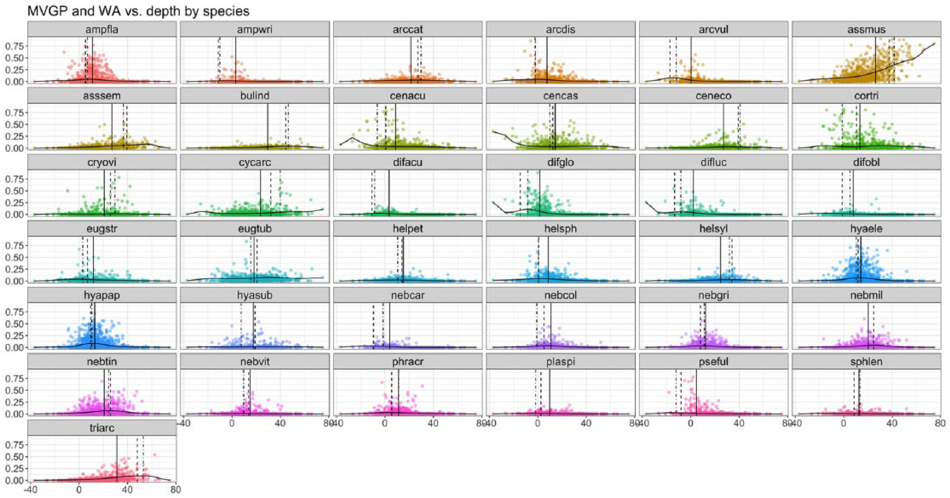
Species abundance versus water-table depth (cm) from the samples in the training dataset (points). The smooth curves are from multivariate Gaussian process for each species. The solid vertical lines are the raw optima from weighted averaging (WA). The dashed vertical lines are the deshrunk WA optima. The dot-dash vertical lines are the coefficients from weighted averaging of partial least squares after five partial least squares components.

MVGP and BUMMER have a few notable features. First, instead of converting counts to proportions, both models begin with compositional count data. It is better to model the data in the manner the data were collected than to transform the data to fit a specific model because data transformations done before the modeling can introduce uncertainty that can be difficult to account for. For example, we know that the compositional count data have variability that is unaccounted for in the traditional models. By modeling the compositional counts with a Dirichlet-multinomial likelihood, the Bayesian hierarchical models are better able to account for the overdispersion observed in the data while automatically satisfying the sum-to-one constraint. MVGP jointly fits a functional relationship between abundance and the covariate using B-splines. The B-spline functional relationship is capable of capturing potentially asymmetric and/or multi-modal responses in a species’ relative abundance along an ecological gradient (Hefley et al., 2017). These potentially more complex functional responses to the covariate are not accommodated by models based on unimodal distributions or a simple mean (i.e. BUMMER, WA, MLRC). There are many potential avenues for modifying these Bayesian models to improve the predictions. Some ideas include accounting for interactions among species, adding spatially/temporally correlated random effects to model overdispersion in the data, and clustering species with similar responses to the environmental covariate to reduce the number of parameters that need to be estimated.

Cross-validation and scoring rules

We use cross-validation to evaluate the performance of all of these models introduced above. Cross-validation consists of five steps: (1) setting aside a subset of the data (the test set), (2) fitting a model using the remaining data (the training set), (3) generating predictions about the test set, (4) evaluating the predictions about the test set, and (5) repeating the process with different test and training sets. In statistics and machine learning, cross-validation performance of a model gives a good indication of the performance of a predictive model on novel data (Hooten and Hobbs, 2015). If a model’s predictions are accurate and precise under cross-validation, then it is generally reasonable to assume that the quality of the predictions will generalize to new data. This generalizability is a critical property in paleoclimate reconstruction because there are often no direct measurements of the covariate of interest for the reconstruction samples. Recent work on transfer function validation has highlighted the usefulness of independent test sets, such as modern samples not included in the training set (Payne et al., 2012; Tsyganov et al., 2016; Van Bellen et al., 2014) or instrumental data (Swindles et al., 2015). In the case where these are unavailable, cross-validation remains the state-of-the-art and is commonly used to evaluate competing models in statistics and machine learning. For this study, no independent test set or instrumental data are available, so we perform a 10-fold cross-validation and use the following scoring rules to evaluate the strengths and weaknesses of the predictions coming from the seven models under comparison

Evaluation of model performance using cross-validation requires a choice of scoring rule. Commonly used scoring rules include MSPE and mean absolute error (MAE). MSPE measures the model’s skill in predicting the mean, while MAE measures skill in predicting the median. Smaller MSPE and MAE indicate better model performance.

A desirable property of a scoring rule is propriety. A scoring rule is proper if the scoring rule chooses the best predictive model on average. In practice, proper scoring rules have a similar interpretation to many other statistical quantities: for any given dataset a proper scoring rule might not pick the best model due to sampling variability, but a proper scoring rule will pick the best predictive model over repeated re-sampling. MSPE and MAE are generally not strictly proper scoring rules because if there are two models with the same predictive mean but different predictive standard deviations, the models will have the same MSPE, but the model with 95% predictive coverage intervals closest to a 95% frequency is the better predictive model. Therefore, MSPE is unable to determine the better predictive model and is not strictly proper. The continuous ranked probability score (CRPS) was developed to be a proper scoring rule that is both accurate (predictive mean is centered on the latent quantity) and precise (the predictive distribution is calibrated so that the $α %$ predictive distribution has empirical coverage near $α %$ (Gneiting, 2011). For the non-Bayesian methods, the CRPS score is equivalent to MAE because these methods do not produce full predictive distributions.

Computing methods

Analyses were done in R (R Core Team, 2017). WA, MLRC, and MAT were fit with the rioja package (Juggins, 2017). RF was fit using the package randomForest (Liaw and Wiener, 2002). BUMMER was fit using Stan (Carpenter et al., 2016). MVGP was fit using the BayesComposition package, available on GitHub at github.com/jtipton25/BayesComposition. The BayesComposition repository also includes code and data to replicate the figures and analyses in this paper.

Results and discussion

Because WA and WAPLS are the most commonly used transfer function methods in the analysis of testate amoebae, we focus our analysis on the performance of WA and WAPLS compared with the Bayesian models, with some brief discussion of the broader suite of models.

Fits to training set

Figure 2 illustrates the model fits to the training dataset by comparing MVGP, WA, and WAPLS. Each taxon’s distribution of abundances is plotted as a function of WTD. The response curves generated by MVGP and the raw WA optima, deshrunk WA optima, and WAPLS optima are plotted for each taxon. The plots of abundance versus WTD illustrate the strongly over-dispersed nature of the data and the difficulty of summarizing these distributions with a simple mean. The distributions of some taxa may be reasonably summarized by an optimal WTD (e.g. Amphitrema wrightianum and Pseudodifflugia fulva–type). The distributions of other species, however, are clearly not well-represented by the WA optima (e.g. Assulina muscorum and Trigonopyxis arcula). For many species, the deshrunk WA optima and the WAPLS-derived coefficient are comparable, but there are many notable differences. For some species (e.g. H. subflava, Nebela collaris-bohemica–type, and others), the WAPLS-derived coefficients are significantly different from what a visual inspection of the distribution might suggest. The species coefficients derived from WAPLS with multiple components (here we are using two PLS components) become no longer interpretable as optima of the ecological distributions. Instead, they are regression coefficients meant to give a better overall prediction of the covariate (Juggins and Birks, 2012).

Cross-validation experiment

We performed a 10-fold cross-validation experiment. Each of the 951 samples in the training set was in the test set for exactly one of the cross-validation folds. Figure 3 shows the observed versus predicted WTDs with a one-to-one line and a linear fit. We also calculated four scoring metrics to numerically evaluate the cross-validation results (Table 1).

Figure 3.

Observed versus predicted water-table depth (cm) for each model from the 10-fold cross-validation experiment on the training dataset of 951 surface testate amoebae assemblages. Red lines in each panel indicate the one-to-one line. Blue lines in each panel are a linear fit of the observed versus predicted WTDs. Error bars denote the 95% credible interval.

Table 1.

Scoring results from 10-fold cross-validation experiment performed on the modern training dataset. Lower scores for MSPE, MAE, and CRPS indicate better performance. For coverage, better performance is indicated by values closer to the nominal rate (in this case, 95%).

	MVGP	BUMMER	WA	WAPLS	MLRC	MAT	RF
MSPE	121.05	111.65	89.99	86.38	193.14	71.99	74.30
MAE	8.32	8.08	7.20	7.02	10.04	6.24	6.22
% CI coverage	75	75	95	98	94	73	95
CRPS	6.27	6.06	7.20	7.02	10.04	6.24	6.22

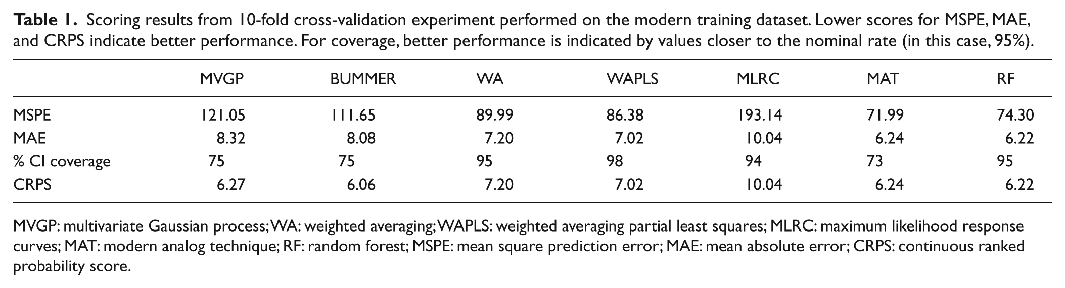
MVGP: multivariate Gaussian process; WA: weighted averaging; WAPLS: weighted averaging partial least squares; MLRC: maximum likelihood response curves; MAT: modern analog technique; RF: random forest; MSPE: mean square prediction error; MAE: mean absolute error; CRPS: continuous ranked probability score.

The results of the cross-validation show a clear bias-variance trade-off in both the plots of observed versus fitted WTD (Figure 3) and in the scores (Table 1). WA, WAPLS, MAT, and RF all show significant bias in the plots of observed versus predicted WTD as evidenced by an offset of the linear fit (blue line) from the one-to-one line (red line). This induced bias, a shrinkage to the mean, allows for generally smaller standard deviations. In contrast, MVGP, BUMMER, and MLRC have smaller bias but larger variance.

This bias-variance tradeoff is also apparent in the cross-validation scores (Table 1). MAT, RF, WA, and WAPLS have the smallest MSPE and MAE (metrics of prediction accuracy for the mean) compared with MLRC, which has the largest MSPE and MAE, and MVGP and BUMMER, which are intermediate.

WA, WAPLS, MLRC, and RF all have 95% credible interval (CI) coverage close to the nominal rate. The Bayesian methods (MVGP and BUMMER) had the lower coverages, approximately 75%, for their 95% CIs. This is likely due to overdispersion in the count data beyond what can be accounted for by the Dirichlet-multinomial likelihood.

For CRPS, the integrated mean and variance score, BUMMER performs best, followed by MVGP, RF, and MAT and then WA and WAPLS. MLRC performs worst.

Will skill in cross-validation generalize to novel data?

The goals of model evaluation under cross-validation are to estimate how well the predictive model can generate predictions on novel data. In our experiment, we consider a variety of methods that have relative predictive strengths and weaknesses. WA, WAPLS, MAT, and RF are generally good predictive methods, but are not based on a statistical likelihood. Thus, their predictive ability does not come with any of the statistical guarantees like the ‘law of large numbers’.

Furthermore, because MAT and RF rely on finding analogs to generate predictions, their predictive skill can only generalize to new data when there are reasonable analogs for the new data in the training set. In cross-validation, this is unlikely to be important, but non-analog issues can become a source of bias when generating predictions downcore. MAT is not widely used for reconstructions with testate amoeba datasets due to these difficulties of finding good analogs downcore (Charman, et al. 2007), but because MAT is still widely used with other sources of compositional data (Marsicek, et al. 2018; Simpson, et al. 2005), we have retained it here for completeness. There are many possible sources of non-analog assemblages, but one potential source for testate amoebae–based reconstructions is differential preservation of certain types of tests (Mitchell et al., 2008). Thus, it is important to check whether there are good analogs for the downcore samples in the training dataset. To do this, we calculated the squared chord distance of the accepted analogs for each sample in the training set in cross-validation and for each sample in the Caribou Bog core. We found that the Caribou Bog samples had systematically worse analogs than the training dataset (Figure 4a). We then looked at these analogs in the time domain and found there is no clear temporal trend in accepted analog distance (Figure 4b), but there does appear to be some serial autocorrelation with some periods having better analogs and some having worse analogs in the training dataset.

Figure 4.

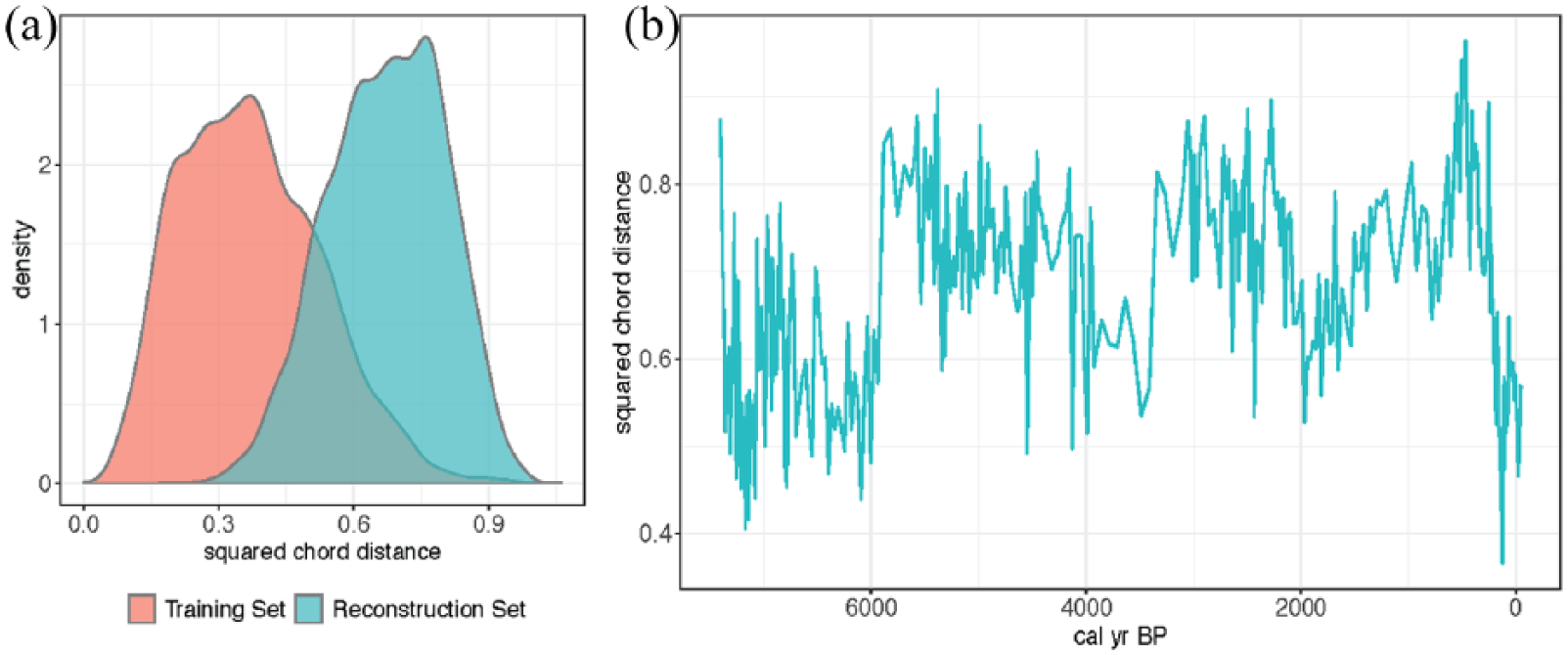
(a) Squared chord distances of the accepted analogs from modern analog technique (MAT) for the training dataset (red) and reconstruction dataset from Caribou Bog (blue). Smaller squared chord distance corresponds to more similar assemblages. The training dataset contains many good analogs for the assemblages within the training dataset (distances for the red density curve are small), whereas the distances of the analog assemblages for the reconstruction dataset are larger and thus not as similar. (b) Time series of the median squared chord distance from the accepted analog assemblages in the training dataset to each assemblage in the Caribou Bog reconstruction dataset. This panel shows temporal evolution of the analogs summarized by the blue density curve in Panel (a).

This analysis provides evidence that the strong predictive skill of MAT, RF, WA, and WAPLS in cross-validation may not generalize to predictive skill in reconstruction, a feature that is common in Quaternary paleoclimate and paleoecology (Jackson, 2012). On the other hand, likelihood-based approaches such as MLRC, MVGP, and BUMMER are capable of generalizing to novel data where there are not appropriate analogs and generating predictions with uncertainties that account for how well the covariate value is known for a given assemblage. From this perspective, likelihood-based methods are a relatively conservative approach to prediction because they are potentially less prone to issues of analog similarity and predictive bias (Tipton et al., 2019).

Reconstruction

We now move from cross-validation, where we have both the testate amoeba assemblage and the measured WTD, to reconstruction. In reconstruction, we only have a testate amoeba assemblage and we wish to estimate a WTD. The 7500 years of testate amoeba assemblages from Caribou Bog are shown in Figure S2 (available online). We then apply the seven transfer function models to infer a WTD history from Caribou Bog. The resulting reconstructions are shown in Figure 5, and the z-scores of the reconstructions are shown in Figure S3 (available online). The methods break out into three subsets. The first subset is formed by the two Bayesian models – MVGP and BUMMER; the resulting reconstructions look similar to each other in terms of both means and uncertainties. The main difference between MVGP and Bummer is the magnitude of some of the smaller deviations. MVGP tends to have a somewhat damped response compared with BUMMER. This damped response could be due to the more flexible ecological responses allowed by MVGP. The uncertainties, as denoted by the 50% and 95% CIs are generally smaller and more variable from sample to sample compared with the other methods. It makes intuitive sense that some predictions should be more certain than others for many potential reasons, including, for example, the particular set of species present and their distributions, the similarity to samples in the training dataset, or the number of individuals counted. With their uncertainties that vary from sample to sample, Bayesian models capture these features of the data.

Figure 5.

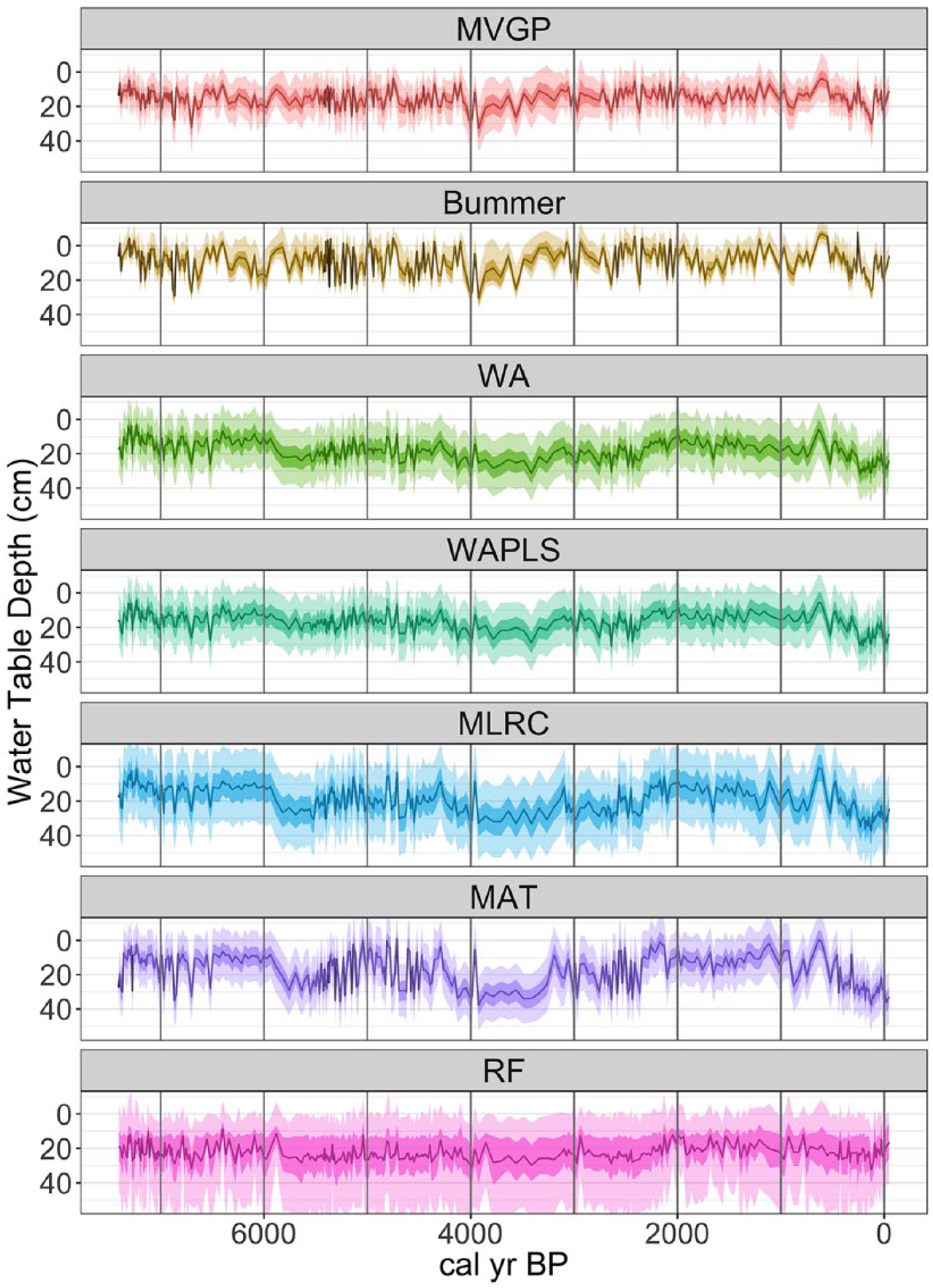
Reconstructions of water-table depth based on testate amoebae assemblages from Caribou Bog. For each panel, the underlying testate amoebae assemblage data are identical; the only thing that changes is the transfer function model. The dark shading denotes 50% credible interval, and the lighter shading denotes 95% credible interval.

The next subset is WA, WAPLS, MLRC, and MAT. The reconstructions for Caribou Bog that result from these WA, MLRC, and MAT all look similar to each other, again with some variability in the magnitude of the changes in WTD. The reconstructed pattern from WAPLS appears to be intermediate between the Bayesian models and WA. For this set of four models, the uncertainties from sample to sample are nearly constant. These unchanging uncertainties are due to the large $v_{2}$ irreducible error component. The $v_{2}$ component is responsible for 98% of the root mean square error of prediction in this dataset. This large irreducible error component limits the usefulness of the uncertainties estimated from these methods.

Finally, RF produces predictions with a mean near the mean of the training dataset, little variability around that mean, and wide uncertainties. This is likely due to the lack of good analogs in the training set for the reconstruction samples as discussed above. The samples with smaller uncertainties for RF (e.g. around 2000 and 6000 yr BP) are associated with samples that have better analogs in the training dataset (Figure 4b).

Inference on past hydrology

To a first order, when the different methods are applied to the same subfossil dataset (Figure S2, available online), the resulting estimates of past hydrological variability are similar (Figure 5; Figure S3, available online). This is reassuring because the underlying data are identical between the different reconstructions, but there are some junctures at which one might draw different inferences depending on the method used to reconstruct WTD. For example, one would infer a significant dry event at ca. 4000 yr BP using MVGP and BUMMER. But using WA, MAT, and other methods, this event is not nearly as pronounced. This divergence is related to differing model responses to an increase in Assulina muscorum. A. muscorum occurs across the moisture gradient, but obtains significantly higher abundance in dry conditions (Figure 2). This affinity for dry conditions leads the Bayesian models to infer drier conditions in response to a small increase in A. muscorum. In contrast, WA does not respond strongly because the percentage increase of A. muscorum is relatively small, and therefore, its influence on the WA reconstruction is small. This event illustrates how MVGP and BUMMER can draw out potentially important single-species anomalies that may be missed by other models. This sensitivity leads to a more complete use of the full assemblage, but it comes with a caveat: we need to carefully consider whether species, like A. muscorum, that can leverage a WTD reconstruction are faithful indicators of the hydrologic status of the peatland. These are testable ecological hypotheses and avenues for future improvement of mechanistic models (e.g. accommodation of more complex relationships between the abundance of certain species and the covariate).

In contrast to the event at 4000 yr BP, at ca. 6000 yr BP, WA, MAT, and MLRC show a large drop in WTD, but MVGP and BUMMER do not. The large change in WTD predicted by WA and others is driven by a change in dominance from Archerella flavum to H. subflava. These species occur in high percentages ( $~ 40 %$ ), and thus, the exchange of the two drives large changes in WTD for WA. However, the change in the dominant species does not drive a large change in the MVGP and BUMMER reconstructions because the difference between the affinities of the two species, when considering their full distribution in this calibration dataset, is relatively small (Figure 2). Numerous modern and paleoecological studies suggest that the shift from A. flavum to H. subflava is a meaningful indicator of a change from wet to dry conditions (e.g. Booth and Jackson, 2003; Charman et al., 1999; Clifford and Booth, 2013; Sullivan and Booth, 2011; Swindles et al., 2009; Talbot et al., 2010), suggesting that the Bayesian methods likely underestimate the covariate response to this change in the testate amoebae assemblage. Incorporating this expert knowledge is possible in the Bayesian hierarchical framework, and future model development should seek to understand and refine the response of these models to changes in dominant species. These two events represent examples of differential sensitivity of different types of transfer function methods. These kinds of differences in reconstructions based on choice of transfer function model are a source of uncertainty that deserves increased attention in paleoenvironmental reconstructions from proxies based on compositional data. Understanding where and why different models diverge can lead to improved inference on both modern ecology and past hydrology.

Conclusions and future directions: Or, Why Bayesian? Why bother?

We have presented a detailed analysis of methods for reconstructing WTD from testate amoebae community composition. We reviewed existing methods and introduced a new Bayesian method and a Bayesian method that had not yet been applied to testate amoebae data. We tested the models in a cross-validation framework and then applied them to reconstructions.

We found that the existing methods compare well in cross-validation with more complex Bayesian models, but for the simpler existing methods we found that their predictive skill in cross-validation may not transfer to skill in reconstruction (Tipton et al., 2019). When we applied the models in reconstruction, we found generally similar inferences of past hydrology with some key differences. We investigated the sources of some of the discrepancies between the reconstructions from different models. Ultimately, when comparing competing models at a single site without an independent target for validation, it is unclear whether one reconstruction is correct and another is wrong. By presenting a systematic comparison of results from different models on the same datasets, we illustrate the importance of model choice as a source of uncertainty in records based on compositional data (Gelman and Loken, 2014; Jackson, 2012).

Bayesian models are worth developing and considering for testate amoebae and other paleoenvironmental proxies based on compositional data. Bayesian models like MVGP and BUMMER are mechanistic models driven primarily by assumptions about the unobserved ecological processes. Developing these types of models makes our assumptions clear and written in the formal language of statistics and can yield improved mechanistic understanding of the system being studied. Mechanistic models underpinned by formal statistics like these are worth the extra effort involved because they allow for a more complete use of the compositional data we spend so much time collecting and result in more robust paleoenvironmental inferences. Including meaningfully estimated uncertainties makes these inferences even more useful. Bayesian models formally account for uncertainty throughout the modeling process (Hobbs and Hooten, 2015). This more complete treatment of uncertainty quantifies how well we really know the past values of the environmental covariate of interest. In secondary analyses and syntheses, uncertainties are necessary to weigh and combine information from many different types of proxies (Hakim et al., 2016; Shuman et al., 2018). When Bayesian models are used on a network of sites, it is possible to add an explicit spatial component to borrow strength across sites and gain new inference on the covariate over space and time with complete uncertainties. With traditional methods, there is a less clear path to achieve a similar borrowing of space and time while properly propagating uncertainty.

We encourage users of all proxies based on compositional data to carefully examine their data and methods in a framework like the one presented here. Testing and comparing new and existing models in a systematic framework leads to a deeper understanding of the strengths and weaknesses of available tools. Regardless of whether the process results in dramatic improvements of inferences, the process itself is clarifying and important: questioning and testing models and assumptions that underlie our important scientific inferences is critical for minimizing ‘ignorance creep’ (Jackson, 2012).

Supplemental Material

FigS1-CaribouAgeModel – Supplemental material for Comparing and improving methods for reconstructing peatland water-table depth from testate amoebae

Supplemental material, FigS1-CaribouAgeModel for Comparing and improving methods for reconstructing peatland water-table depth from testate amoebae by Connor Nolan, John Tipton, Robert K Booth, Mevin B Hooten and Stephen T Jackson in The Holocene

Supplemental Material

FigS2_TA_data – Supplemental material for Comparing and improving methods for reconstructing peatland water-table depth from testate amoebae

Supplemental material, FigS2_TA_data for Comparing and improving methods for reconstructing peatland water-table depth from testate amoebae by Connor Nolan, John Tipton, Robert K Booth, Mevin B Hooten and Stephen T Jackson in The Holocene

Supplemental Material

FigS3_zscores_allmodels – Supplemental material for Comparing and improving methods for reconstructing peatland water-table depth from testate amoebae

Supplemental material, FigS3_zscores_allmodels for Comparing and improving methods for reconstructing peatland water-table depth from testate amoebae by Connor Nolan, John Tipton, Robert K Booth, Mevin B Hooten and Stephen T Jackson in The Holocene

Supplemental Material

TableS1-Caribou14Cdates – Supplemental material for Comparing and improving methods for reconstructing peatland water-table depth from testate amoebae

Supplemental material, TableS1-Caribou14Cdates for Comparing and improving methods for reconstructing peatland water-table depth from testate amoebae by Connor Nolan, John Tipton, Robert K Booth, Mevin B Hooten and Stephen T Jackson in The Holocene

Footnotes

Acknowledgements

This work is part of the Paleoecological Observatory Network (PalEON) Project (). It was funded by the National Science Foundation Macrosystems Biology program under grant nos. DEB-1241851 and DEB-1241856. We thank Melissa Berke for field assistance; Tom Webb for historical perspective on the development of transfer functions; and Don Charles, Dan Charman, and an anonymous reviewer for useful comments that improved the manuscript. Any use of trade, firm, or product names is for descriptive purposes only and does not imply endorsement by the US Government.

Funding

The author(s) received no financial support for the research, authorship, and/or publication of this article.

Supplemental material

Supplemental material for this article is available online.

ORCID iD

Connor Nolan

References

Amesbury

Swindles

Bobrov

, et al. (2016) Development of a new pan-European testate amoeba transfer function for reconstructing peatland palaeohydrology. Quaternary Science Reviews 152: 132–151.

Battarbee

(1984) Diatom analysis and the acidification of lakes. Philosophical Transactions of the Royal Society of London. Series B, Biological Sciences 305(1124): 451–477.

Battarbee

Jones

Flower

, et al. (2002) Diatoms. In: Smol

(ed.) Tracking Environmental Change Using Lake Sediments. New York: Springer, pp. 155–202.

Birks

HJB

(1998) Numerical tools in palaeolimnology – Progress, potentialities, and problems. Journal of Paleolimnology 20(4): 307–332.

Birks

HJB

Simpson

(2013) ‘Diatoms and pH reconstruction’(1990) revisited. Journal of Paleolimnology 49(3): 363–371.

Birks

HJB

ter Braak

Line

, et al. (1990) Diatoms and pH reconstruction. Philosophical Transactions of the Royal Society of London. Series B, Biological Sciences 327(1240): 263–278.

Booth

(2002) Testate amoebae as paleoindicators of surface-moisture changes on Michigan peatlands: Modern ecology and hydrological calibration. Journal of Paleolimnology 28(3): 329–348.

Booth

(2008) Testate amoebae as proxies for mean annual water-table depth in Sphagnum-dominated peatlands of North America. Journal of Quaternary Science 23(1): 43–57.

Booth

(2010) Testing the climate sensitivity of peat-based paleoclimate reconstructions in mid-continental North America. Quaternary Science Reviews 29(5–6): 720–731.

10.

Booth

Jackson

(2003) A high-resolution record of late-Holocene moisture variability from a Michigan raised bog, USA. The Holocene 13(6): 863–876.

11.

Booth

Zygmunt

(2005) Biogeography and comparative ecology of testate amoebae inhabiting sphagnum-dominated peatlands in the Great Lakes and Rocky Mountain regions of North America. Diversity and Distributions 11(6): 577–590.

12.

Booth

Hotchkiss

Wilcox

(2005) Discoloration of polyvinyl chloride (PVC) tape as a proxy for water-table depth in peatlands: Validation and assessment of seasonal variability. Functional Ecology 19(6): 1040–1047.

13.

Breiman

(2001) Random forests. Machine Learning 45(1): 5–32.

14.

Carpenter

Gelman

Hoffman

, et al. (2016) Stan: A probabilistic programming language. Journal of Statistical Software 20(2): 1–37.

15.

Charles

(1985) Relationships between surface sediment diatom assemblages and lakewater characteristics in Adirondack lakes. Ecology 66(3): 994–1011.

16.

Charman

Blundell

and ACCROTELM members (2007) A new European testate amoebae transfer function for palaeohydrological reconstruction on ombrotrophic peatlands. Journal of Quaternary Science 22(3): 209–221.

17.

Charman

Hendon

Packman

(1999) Multiproxy surface wetness records from replicate cores on an ombrotrophic mire: Implications for Holocene palaeoclimate records. Journal of Quaternary Science 14(5): 451–463.

18.

Clifford

Booth

(2013) Increased probability of fire during late Holocene droughts in northern New England. Climatic Change 119(3–4): 693–704.

19.

Davis

Anderson

Berge

(1985) Palaeolimnological evidence that lake acidification is accompanied by loss of organic matter. Nature 316(6027): 436.

20.

Edwards

Fyfe

Jackson

(2017) The first 100 years of pollen analysis. Nature Plants 3: 17001.

21.

Gajewski

(1987) Environmental history of Caribou Bog, Penobscot Co., Maine. Naturaliste Canadien 114: 133–140.

22.

Gauch

Whittaker

(1972) Coenocline simulation. Ecology 53(3): 446–451.

23.

Gelman

Loken

(2014) The Statistical Crisis in Science. American Scientist. 102: 460–465.

24.

Gelman

Simpson

Betancourt

(2017) The prior can often only be understood in the context of the likelihood. Entropy 19(10): 555.

25.

Gneiting

(2011) Making and evaluating point forecasts. Journal of the American Statistical Association 106(494): 746–762.

26.

Goring

Williams

Blois

, et al. (2012) Deposition times in the northeastern United States during the Holocene: Establishing valid priors for Bayesian age models. Quaternary Science Reviews 48: 54–60.

27.

Hakim

Emile-Geay

Steig

, et al. (2016) The last millennium climate reanalysis project: Framework and first results. Journal of Geophysical Research: Atmospheres 121(12): 6745–6764.

28.

Hefley

Broms

Brost

, et al. (2017) The basis function approach for modeling autocorrelation in ecological data. Ecology 98(3): 632–646.

29.

Hobbs

Hooten

(2015) Bayesian Models: A Statistical Primer for Ecologists. Princeton, NJ: Princeton University Press.

30.

Hoeting

Madigan

Raftery

, et al. (1999) Bayesian model averaging: A tutorial. Statistical Science 14: 382–401.

31.

Hooten

Hobbs

(2015) A guide to Bayesian model selection for ecologists. Ecological Monographs 85(1): 3–28.

32.

Davis

(1995) Postglacial development of a Maine bog and paleoenvironmental implications. Canadian Journal of Botany 73(4): 638–649.

33.

Hustedt

(1939 [1937]) Systematische und ökologische unter-suchungen über die diatomeen-flora von Java, Bali und Sumatra nach dem material der deutschen limnologischen Sunda-Expedition. I. Archives of Hydrobiology 37: 15–16.

34.

Hydro2k

(2017) Comparing proxy and model estimates of hydroclimate variability and change over the Common Era. Climate of the past 13(12): 1851–1900.

35.

Imbrie

Kipp

(1971) A new micropaleontologial method for quantitative paleoclimatology: Application to a late Pleistocene Caribbean core. In: Flint

(ed.) The Late Cenozoic Glacial Ages. New Haven, CT: Yale University Press, pp. 71–181.

36.

Imbrie

Webb

(1981) Transfer functions: Calibrating micropaleontological data in climatic terms. In: Berger

(ed.) Climatic Variations and Variability: Facts and Theories. New York: Springer, pp. 125–134.

37.

Imbrie

Van Donk

Kipp

(1973) Paleoclimatic investigation of a late pleistocene Caribbean Deep-Sea Core: Comparison of isotopic and faunal methods 1. Quaternary Research 3(1): 10–38.

38.

Iversen

(1944) Viscum, Hedera and Ilex as climate indicators: A contribution to the study of the post-glacial temperature climate. Geologiska Föreningen I Stockholm Förhandlingar 66(3): 463–483.

39.

Jackson

(2012) Representation of flora and vegetation in Quaternary fossil assemblages: Known and unknown knowns and unknowns. Quaternary Science Reviews 49: 1–15.

40.

Jackson

Williams

(2004) Modern analogs in Quaternary paleoecology: Here today, gone yesterday, gone tomorrow? Annual Review of Earth and Planetary Sciences 32: 495–537.

41.

Juggins

(2013) Quantitative reconstructions in palaeolimnology: New paradigm or sick science? Quaternary Science Reviews 64: 20–32.

42.

Juggins

(2017) Rioja: Analysis of Quaternary Science Data (R package version 0.9-15.1). Available at: http://www.staff.ncl.ac.uk/stephen.juggins/.

43.

Juggins

Birks

HJB

(2012) Quantitative environmental reconstructions from biological data. In: Smol

(ed.) Tracking Environmental Change Using Lake Sediments. New York: Springer, pp. 431–494.

44.

Liaw

Wiener

(2002) Classification and regression by randomForest. R News 2(3): 18–22.

45.

Markel

Booth

Qin

(2010) Testate amoebae and δ13c of Sphagnum as surface-moisture proxies in Alaskan peatlands. The Holocene 20(3): 463–475.

46.

Marlon

Pederson

Nolan

, et al. (2017) Climatic history of the northeastern United States during the past 3000 years. Climate of the Past 13(10): 1355.

47.

Marsicek

Shuman

Bartlein

, et al. (2018) Reconciling divergent trends and millennial variations in Holocene temperatures. Nature 554(7690): 92.

48.

Mitchell

Payne

Lamentowicz

(2008) Potential implications of differential preservation of testate amoeba shells for paleoenvironmental reconstruction in peatlands. Journal of Paleolimnology 40(2): 603–618.

49.

Nygaard

(1956) Ancient and recent ﬂora of diatoms and chrysophyceae in Lake Gribso. Studies on the humic acid Lake Gribso. Folia Limnologica Scandinavica 8: 32–94.

50.

Oehlert

(1988) Interval estimates for diatom-inferred lake pH histories. Canadian Journal of Statistics 16(1): 51–60.

51.

Oksanen

Läärä

Huttunen

, et al. (1990) Maximum likelihood prediction of lake acidity based on sedimented diatoms. Journal of Vegetation Science 1(1): 49–56.

52.

Overpeck

Webb

Prentice

(1985) Quantitative interpretation of fossil pollen spectra: Dissimilarity coefficients and the method of modern analogs. Quaternary Research 23(1): 87–108.

53.

Parnell

(2014) Bchron: Radiocarbon dating, age-depth modelling, relative sea level rate estimation, and non-parametric phase modelling. R Package Version 4(1). Available at: https://rdrr.io/cran/Bchron/.

54.

Payne

Mitchell

(2009) How many is enough? Determining optimal count totals for ecological and palaeoecological studies of testate amoebae. Journal of Paleolimnology 42(4): 483–495.

55.

Payne

Telford

Blackford

, et al. (2012) Testing peatland testate amoeba transfer functions: Appropriate methods for clustered training-sets. The Holocene 22(7): 819–825.

56.

Phleger

(1953) North Atlantic core foraminifera. Reports on the Swedish Deep-sea Expedition. Available at: https://www.researchgate.net/publication/290456865_North_Atlantic_Core_Foraminifera_Collected_by_Swedish_Deep-Sea_Expedition_ABSTRACT.

57.

Prentice

(1980) Multidimensional scaling as a research tool in quaternary palynology: A review of theory and methods. Review of Palaeobotany and Palynology 31: 71–104.

58.

R Core Team (2017) R: A Language and Environment for Statistical Computing. R Foundation for Statistical Computing, Vienna, Austria. Available at: https://www.R-project.org/.

59.

Renberg

Hellberg

Nilsson

(1985) Effects of acidification on diatom communities as revealed by analyses of lake sediments. Ecological Bulletins 37: 219–223.

60.

Salonen

Ilvonen

Seppä

, et al. (2012) Comparing different calibration methods (WA/WA-PLS regression and Bayesian modelling) and different-sized calibration sets in pollen-based quantitative climate reconstruction. The Holocene 22(4): 413–424.

61.

Schapire

(1990) The strength of weak learnability. Machine Learning 5(2): 197–227.

62.

Shuman

Routson

McKay

, et al. (2018) Placing the Common Era in a Holocene context: Millennial-to-centennial patterns and trends in the hydroclimate of North America over the past 2000 years. Climate of the Past 14: 665–686.

63.

Simpson

Shilland

Winterbottom

, et al (2005) Defining reference conditions for acidified waters using a modern analogue approach. Environmental Pollution 137(1): 119–133.

64.

Smol

(2009) Pollution of Lakes and Rivers: A Paleoenvironmental Perspective. Hoboken, NJ: John Wiley & Sons.

65.

Sullivan

Booth

(2011) The potential influence of short-term environmental variability on the composition of testate amoeba communities in Sphagnum peatlands. Microbial Ecology 62(1): 80–93.

66.

Swindles

Charman

Roe

, et al. (2009) Environmental controls on peatland testate amoebae (Protozoa: Rhizopoda) in the North of Ireland: Implications for Holocene palaeoclimate studies. Journal of Paleolimnology 42(1): 123–140.

67.

Swindles

Holden

Raby

, et al. (2015) Testing peatland water-table depth transfer functions using high-resolution hydrological monitoring data. Quaternary Science Reviews 120: 107–117.

68.

Talbot

Richard

Roulet

, et al. (2010) Assessing long-term hydrological and ecological responses to drainage in a raised bog using paleoecology and a hydrosequence. Journal of Vegetation Science 21(1): 143–156.

69.

Telford

Birks

(2009) Evaluation of transfer functions in spatially structured environments. Quaternary Science Reviews 28(13–14): 1309–1316.

70.

Telford

Andersson

Birks

, et al. (2004) Biases in the estimation of transfer function prediction errors. Paleoceanography 19(4): 01072.

71.

ter Braak

Juggins

(1993) Weighted averaging partial least squares regression (WA-PLS): An improved method for reconstructing environmental variables from species assemblages. In: Proceedings of the twelfth international diatom symposium, Renesse, 30 August–5 September, pp. 485–502. New York: Springer.

72.

ter Braak

Van Dam

(1989) Inferring pH from diatoms: A comparison of old and new calibration methods. Hydrobiologia 178(3): 209–223.

73.

Tipton

Hooten

Nolan

, et al. (2019) Predicting paleoclimate from compositional data using multivariate Gaussian process inverse prediction. arXiv: 1903.05036

74.

Toivonen

Mannila

Korhola

, et al. (2001) Applying Bayesian statistics to organism-based environmental reconstruction. Ecological Applications 11(2): 618–630.

75.

Trachsel

Telford

(2016) Estimating unbiased transfer-function performances in spatially structured environments. Climate of the past 12(5): 1215–1223.

76.

Tsyganov

Mityaeva

Mazei

, et al. (2016) Testate amoeba transfer function performance along localised hydrological gradients. European Journal of Protistology 55: 141–151.

77.

Van Bellen

Mauquoy

Payne

, et al. (2014) Testate amoebae as a proxy for reconstructing Holocene water table dynamics in southern Patagonian peat bogs. Journal of Quaternary Science 29(5): 463–474.

78.

Van Bellen

Mauquoy

Payne

, et al. (2017) An alternative approach to transfer functions? Testing the performance of a functional trait-based model for testate amoebae. Palaeogeography, Palaeoclimatology, Palaeoecology 468: 173–183.

79.

Von Post

(1918) Forest tree pollen in south Swedish peat bog deposits, translated by Margaret B. Davis and Knut Faegri, 1967. Pollen Et Spores 9: 375–401.

80.

Warner

Charman

(1994) Holocene changes on a peatland in northwestern Ontario interpreted from testate amoebae (Protozoa) analysis. Boreas 23(3): 270–279.

81.

Webb

Bryson

(1972) Late-and postglacial climatic change in the northern Midwest, USA: Quantitative estimates derived from fossil pollen spectra by multivariate statistical analysis. Quaternary Research 2(1): 70–115.

82.

Woodland

Charman

Sims

(1998) Quantitative estimates of water tables and soil moisture in Holocene peatlands from testate amoebae. The Holocene 8(3): 261–273.

83.

Wright

Mann

Glaser

(1984) Piston corers for peat and lake sediments. Ecology 65(2): 657–659.

84.

Wright

Winter

Patten

(1963) Two pollen diagrams from southeastern Minnesota: Problems in the regional late-glacial and postglacial vegetational history. Geological Society of America Bulletin 74(11): 1371–1396.

Supplementary Material

Please find the following supplemental material available below.

For Open Access articles published under a Creative Commons License, all supplemental material carries the same license as the article it is associated with.

For non-Open Access articles published, all supplemental material carries a non-exclusive license, and permission requests for re-use of supplemental material or any part of supplemental material shall be sent directly to the copyright owner as specified in the copyright notice associated with the article.

0.00 MB

0.50 MB

0.12 MB

0.83 MB

0.05 MB