Mid-Holocene drylands: A multi-model analysis using Paleoclimate Modelling Intercomparison Project Phase III (PMIP3) simulations

Abstract

This study examines changes in aridity levels during the mid-Holocene (approximately 6000 cal. yr ago) using multi-model simulations from the Paleoclimate Modelling Intercomparison Project Phase III. Overall, there is little difference in the total area of drylands from the preindustrial period; global drylands are 8% wetter than during the preindustrial period as measured by an aridity index; and 16% of preindustrial drylands convert to a wetter climate subtype, double the sum of zones that are replaced by a drier category. Considerable variations are present among regions with major contractions of each dryland subtype from northern Africa to South Asia and the main expansions of arid, semiarid, and dry subhumid climates in southern hemisphere continents. The difference in precipitation is the leading factor of the aforementioned changes. The second factor is the altered potential evapotranspiration as mainly induced by relative humidity, which contributes to additional aridity changes in a same direction as precipitation does. The collective effects of precipitation and relative humidity account for more than 80% of the dryland variations. In comparison, the simulated aridity change is in reasonable agreement with reconstructions, while there are model–data discrepancies for Australia and uncertainties across proxies for southern Africa.

Keywords

dryland global mid-Holocene model–data comparison paleoclimate modeling

Introduction

Drylands, which include desert, grassland, and savanna woodland biomes, are characterized by long-term water scarcities and are shaped by high climatic variability, frequent drought, and land degradation (Gaur and Squires, 2018). Roughly one third of the world’s population inhabit drylands (Safriel et al., 2005), whose ecosystems are sensitive to climate change. Both observations and simulations reveal that drylands have expanded in the past 60 years, and the warming trend of drylands is double that of humid regions (Huang et al., 2016a, 2016b). In the 21st century, drylands are projected to expand with continuing global warming (Feng and Fu, 2013), which increases the risk of heat waves and droughts and thus negatively affects agriculture and food security (Sidahmed, 2018). Therefore, it is important to understand both what controls dryland changes under varying climate scenarios and how desertification may be addressed. However, it is impossible to test large climatic fluctuations based solely on the data from an instrumental period whose climate change is relatively temperate. Here, we analyze the mid-Holocene (approximately 6000 yr BP), because its climate differed largely from the present day, and its paleo-data are relatively abundant (Braconnot et al., 2012).

Drylands experience long-term moisture deficits or aridity, the degree of which is affected by various meteorological parameters, including precipitation, heat, and aerodynamics (Middleton and Thomas, 1997). Terrestrial moisture conditions have been inferred for the mid-Holocene using abundant geological records, such as pollen, diatoms, speleothems, dunes, and geomorphic and stratigraphic records. Compared to the present day, the most dramatic wetting occurs in northern Africa and the Arabian Peninsula where steppe and savanna occupy a primary position in the absence of deserts (Hoelzmann et al., 1998). In addition, wetting has also been found in northern India (Dixit and Bera, 2011; Enzel et al., 1999; Singh et al., 1990), eastern Asia (Jiang et al., 2013; Yu et al., 2000; Yu et al., 2001), the southwestern United States (Harrison et al., 2003; Ruter et al., 2004), Central America (Ruter et al., 2004), and northernmost South America (Haug et al., 2001), whereas the opposite holds for the southeastern United States (Bartlein et al., 2011; Ruter et al., 2004) and to the south of northernmost South America (Baker et al., 2001; Behling, 2002; Mayle et al., 2000). Note first that these paleo-data have manifested uncertainties in association with chronologies, methodologies, and data interpretations. For example, there is still disagreement about whether the climate is drier or wetter across northern Australia (Haberle, 2005; Lough et al., 2014; Pickett et al., 2004; Wyrwoll and Miller, 2001), southern Africa, and Europe (Bartlein et al., 2011; Kohfeld and Harrison, 2000). Second, the site-based data still experience spatial scarcities and ambiguity about the extent to which they can represent large-scale features, and it remains unresolved how to upscale the reconstructed data from the single-site to regional scale. Third, the data depict only climate features and seldom involve direct mechanisms. The numerical experiment undertaken by climate models offers an opportunity to address physical explanations on large scales.

A number of numerical experiments have been conducted to investigate mid-Holocene changes in precipitation that are linked to global monsoons (Jiang et al., 2015; Liu et al., 2004; Zhao and Harrison, 2012), hydrological cycles at regional or hemispheric scales (Bosmans et al., 2012; Mantsis et al., 2013; Marshall and Lynch, 2006), and internal feedbacks (Harrison et al., 2003; Marzin and Braconnot, 2009; Zhao et al., 2005). On a large scale, these studies reach a consensus that precipitation increases in northern monsoonal regions and decreases in southern Africa and South America, whereas there remains an ongoing debate as to whether the ocean feedback-induced enhancement of the Australia monsoon reverses the orbitally induced suppression of precipitation (Liu et al., 2004; Mantsis et al., 2013; Marshall and Lynch, 2006; Zhao and Harrison, 2012). However, little attention has been given to the alteration of drylands, including their spatial distribution and degree of aridity, which is not solely determined by precipitation (Middleton and Thomas, 1997).

In the present analysis, we highlight dryland changes during the mid-Holocene and their underlying mechanisms. A quantitative aridity index (AI), as defined by the ratio of annual precipitation to potential evapotranspiration (PET), is employed to map drylands, where the PET is estimated using the Penman–Monteith equation (Allen et al., 1998). The AI used to produce the dryland map is sourced from national organizations, such as the United Nations Educational, Scientific and Cultural Organization (UNESCO) and the United Nations Environment Program (UNEP) (Middleton and Thomas, 1997; UNESCO, 1979). At the large scale, the dryland map produced using the AI matches well with surface vegetation types (Huang et al., 2016a). The analysis is based on climate simulations conducted as part of the Paleoclimate Modelling Intercomparison Project Phase III (PMIP3) project and aims to (1) examine the changes in aridity and spatial distributions of drylands, (2) explore mechanisms responsible for dryland changes, and (3) qualitatively evaluate if the simulations are reconciled with paleo-records. The following section presents the data and method. Aridity changes produced by models are provided in ‘Aridity in simulations’, followed by proxy-based inferences in ‘Aridity in paleo-data’. ‘Discussion’ provides a discussion and conclusions.

Data and method

Model and observation data

In our analysis, monthly mean precipitation, near-surface outputs of daily minimum, maximum, and mean air temperatures, wind speed, and specific humidity or relative humidity, as well as surface outputs of air pressure and latent and sensible heat fluxes, are required to compute the AI. The analysis is based on nine general circulation models participating in the PMIP3 experiments (Table 1), which are used to conduct the mid-Holocene experiment and include all the variables required for the AI computation. The simulations have run long enough with predefined stable boundary conditions (Table 2) to reach a quasi-equilibrium, and the final 30 years are taken to represent the climatology for the preindustrial and mid-Holocene periods. Relative to the preindustrial period, the primary forcing during the mid-Holocene lies in orbital parameters (Berger, 1978), which can be precisely calculated; as a result, the mean annual insolation increased at high latitudes and slightly decreased in the tropics of both hemispheres. The atmospheric greenhouse gas concentrations assigned to the preindustrial control experiment are at levels from approximately 1750 and are slightly changed for the mid-Holocene experiment, resulting in a negligible difference in radiative forcing relative to the orbitally induced change in insolation (Bosmans et al., 2012). More details on the models and associated boundary conditions are available online at http://pmip3.lsce.ipsl.fr/. We emphasize the multi-model medians in the following analysis, as the median field can avoid individual outliers and generally outperforms individual models in a collection of models (Gleckler et al., 2008). Toward a measure of uncertainties of simulations relevant to varying model resolutions and structures, two statistics are presented: (1) the number of models agreeing on the sign of the change and (2) the ratio of inter-model spread, as indicated by the interquartile range, to the absolute value of the multi-model median. A high ratio represents large disagreement across models.

Table 1.

Basic information of PMIP3 models considered in this study.

	Model ID	Modeling center (or group)	Atmospheric resolution	Length of run (years)
	Model ID	Modeling center (or group)	Atmospheric resolution	PI	MH
M1	BCC-CSM1-1	Beijing Climate Center, China	−2.8° × 2.8°, L26	PI	MH	500	100
M2	CNRM-CM5^a	Center National de Recherches Météorologiques, France	−1.4° × 1.4°, L31	850	200
M3	CSIRO-Mk3-6-0^a	Commonwealth Scientific and Industrial Research, Australia	1.875° × −1.9°, L18	500	100
M4	FGOALS-s2	Institute of Atmospheric Physics, CAS, China	−2.8° × 3°−6°, L26	500	100
M5	GISS-E2-R	NASA Goddard Institute for Space Studies, US	2.5° × 2°, L40	1200	100
M6	HadGEM2-CC	Met Office Hadley Center, UK	1.875° × 1.25°, L60	240	35
M7	HadGEM2-ES	Met Office Hadley Center, UK	1.875° × 1.25°, L38	577	102
M8	MIROC-ESM	Japan Agency for Marine-Earth Science and Technology, Japan	−2.8° × 2.8°, L80	630	100
M9	MRI-CGCM3^a	Meteorological Research Institute, Japan	1.125° × −1.1°, L48	500	100

PMIP3: Paleoclimate Modelling Intercomparison Project Phase III.

Indicates the three fully coupled atmosphere–ocean models (AOGCMs), while the other six are fully coupled atmosphere–ocean–vegetation models (AOVGCMs).

The first run is used if the model has multiple runs. The preindustrial and mid-Holocene are in order referred to as PI and MH in the table.

Table 2.

PMIP3 boundary conditions for the preindustrial control and mid-Holocene experiments as taken from PMIP3 website: http://pmip3.lsce.ipsl.fr/.

Boundary conditions	Preindustrial control	Mid-Holocene
Orbital parameters	(ecc = 0.016724) (obl = 23.446°) (peri − 180° = 102.04°)	(ecc = 0.018682) (obl = 24.105°) (peri − 180° = 0.87°)
Solar constant	1365 W m⁻²
Date of vernal equinox	21 March at noon
Greenhouse gases	(CO₂ = 280 ppm) (CH₄ = 760 ppb) (N₂O = 270 ppb)	(CO₂ = 280 ppm) (CH₄ = 650 ppb) (N₂O = 270 ppb)
Vegetation	Fixed at present state in AOGCMs or interactive in AOVGCMs
Ice sheets	Modern
Topography and coastlines	Modern

PMIP3: Paleoclimate Modelling Intercomparison Project Phase III.

The model’s ability to simulate modern aridity is assessed using long-term mean observations and reanalysis data (hereafter both types are referred to as observations) for the period 1981–2010. The precipitation data are taken from the Precipitation Reconstruction over Land (PREC/L) dataset, which is derived from gauge observations from over 17,000 stations and performs well in describing mean distributions of precipitation (Chen et al., 2002). Data for calculating PET are obtained from the National Centers for Environment Prediction – Department of Energy (NCEP–DOE) Atmospheric Model Intercomparison Project (AMIP-II) reanalysis (NCEP-2) (Kanamitsu et al., 2002). All data from simulations and observations are interpolated into the same spatial grids with a horizontal resolution of 0.5° (longitude) × 0.5° (latitude) using bilinear interpolation.

Definition and subtypes of drylands

Drylands are commonly identified based on the AI (Middleton and Thomas, 1997), which is defined as follows:

AI = \frac{P}{PET}

(1)

where P is the annual precipitation, and the unit of P and PET is mm day⁻¹. Precipitation and PET represent the water supply to the land and evaporative demand, respectively, which collectively determine the degree of water deficit or aridity that drylands experience. According to the World Atlas of Desertification from the UNEP (Middleton and Thomas, 1997), drylands are identified as areas with an AI less than 0.65 and are subdivided into four subtypes of hyperarid (AI < 0.05), arid (0.05 ⩽ AI < 0.20), semiarid (0.20 ⩽ AI < 0.50), and dry subhumid (0.50 ⩽ AI < 0.65) regions, whereas regions with an AI higher than 0.65 have a categorically humid climate.

PET estimation

PET measures the sum of evaporation and plant transpiration from a surface with sufficient water and is determined only by meteorological factors. Here the PET is calculated using the Penman–Monteith equation because of its practicality. This equation provides a physically based semi-empirical solution for the PET estimation and is recommended by the Food and Agriculture Organization of the United Nations (FAO) as the sole standard method (Allen et al., 1998). The equation is as follows:

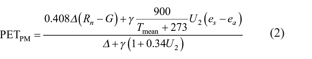
P E T_{P M} = \frac{0.408 Δ (R_{n} - G) + γ \frac{900}{T_{m e a n} + 273} U_{2} (e_{s} - e_{a})}{Δ + γ (1 + 0.34 U_{2})}

(2)

where R_n is the net radiation at the evaporative surface (MJ m⁻² day⁻¹), G is the soil heat flux density (MJ m⁻² day⁻¹), T_mean is the mean daily air temperature at 2 m (°C), U₂ is the wind speed at 2 m (m s⁻¹), e_s is the surface saturation vapor pressure (kPa), e_a is the actual vapor pressure (kPa), γ is the psychometric constant (kPa °C⁻¹), and Δ is the slope vapor pressure curve (kPa °C⁻¹).

The equation considers the combined controls of heat (temperature and radiation) and aerodynamic (vapor pressure deficits and wind speeds) factors. Heat factors supply the vaporizing energy, whereas aerodynamic terms help to remove vapors from the surface for sustaining the evaporation process. The calculating steps have been provided in the FAO-56 guideline (Allen et al., 1998), and several points need to be noted. First, T_mean represents the average of daily maximum and minimum temperatures, and e_s is calculated using the average of saturation vapor pressure at daily maximum and minimum temperatures. Second, given that soil heat flux is not available in model outputs, available energy (AE: R_n − G) is replaced by the sum of sensible and latent heat (Allen et al., 1998; Fu and Feng, 2014). We consider the general energy balance for an evaporating body as follows:

L E = R_{n} - G - H + A_{w} - \frac{Δ Q}{Δ t}

(3)

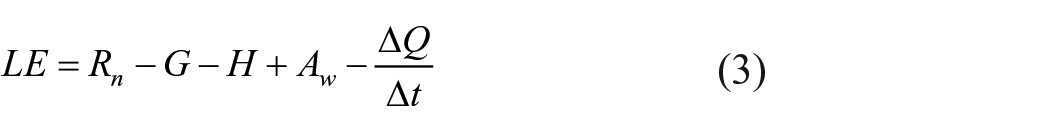
where LE and H are latent and sensible heat at the surface, respectively, A_w is the energy advection, ΔQ/Δt is the temporal change in the heat stored in the body between the beginning and end of Δt, and their units are MJ m⁻² day⁻¹. For an evaporating surface, two latter terms are negligible; thus, the term (R_n − G) can be approximated by (LE + H). Third, e_a can be estimated using the mean relative humidity, dew point temperature or specific humidity. Considering the limitation that none of the three variables are simultaneously present in both simulated and observed datasets, we calculate e_a using the relative humidity for simulations and the specific humidity for observations. Dew point temperature can be approximated by the daily minimum temperature, which makes it possible to calculate e_a using the same variable in both types of data; in arid regions, however, this approximation may lead to noteworthy overstatements of dew point temperature. Finally, note that the surface resistance (r_s), which describes the resistance of vapor flow through stomata openings, total leaf area, and soil surface, is fixed in the FAO-56 standard method (Hobbins et al., 2016), although it is now known to be changed with CO₂ concentration and temperature (Scheff, 2019). Regarding this issue, one recent work (Yang et al., 2019) has provided a simple modification of r_s by making it coupled to the changing CO₂ concentration. However, from the preindustrial period to the mid-Holocene, the CO₂ concentration is kept unchanged in the PMIP3 (Table 2), and global annual temperature is slightly different (Braconnot et al., 2012), thus the constant setting of r_s used here is expected to have little impact on the final result.

Aridity in simulations

Model performance in the modern era

Toward an assessment of the performance of models, we first compare the simulated area and distribution of drylands during the preindustrial period (Figure 1a) to the observed one (Figure 1b) calculated using variables from NCEP-2 (Kanamitsu et al., 2002) and PREC/L (Chen et al., 2002) for the period 1981–2010. In the observations, hyperarid, arid, semiarid, and dry subhumid areas cover 5%, 11%, 13%, and 5% of the earth’s land surface (1.5 × 10⁸ km²), respectively. Hyperarid lands occupy northern Africa, the central Andes, and small parts of the Arabian Peninsula; arid and semiarid zones are widely distributed along the western coasts of the subtropical Americas, northern and southern Africa, the Arabian Peninsula, western India, central Asia, and Australia; dry subhumid regions appear only on the edges of drylands. Such a distribution agrees with previous documentation (Middleton and Thomas, 1997) and matches with varying types of surface vegetation, that is, barren, open shrublands, savannas, and grasslands (Feng and Fu, 2013). The simulated areas of hyperarid, arid, semiarid, and dry subhumid zones average 7%, 9%, 12%, and 6% of the total land area, respectively, which approximate the observations. Spatially, the multi-model median of PMIP3 simulations is broadly consistent with observations on a large scale, although it underestimates the dryland extent over North America and Northwest China and overestimates hyperarid zones from northern Africa to the Arabian Peninsula. Furthermore, the degree of correspondence between simulated and observed fields is measured using the method provided by Taylor (2001). According to this method, three statistics, the spatial correlation coefficient, the normalized standard deviation, and the normalized centered root-mean-square difference between the simulated and PREC/L precipitation or the simulated and NCEP-2 PET, are calculated based on data at all terrestrial grids from 60°S to 60°N. Briefly, if the former two statistics are closer to 1, namely the last statistic is closer to 0, the simulation better approximates the observation. The Taylor diagram (Figure S1 available online) illustrates the three statistics for individual models (the median field) follow the order 0.77–0.90 (0.90), 0.99–1.56 (1.19), and 0.45–0.95 (0.53) for PET and 0.72–0.85 (0.87), 0.71–1.30 (0.89), and 0.56–0.84 (0.50) for precipitation, indicating that the models capture the main features of the spatial pattern and the variation amplitude of the observed precipitation and PET climatology. The multi-model median is superior to most individual models and is therefore used as the best simulation.

Figure 1.

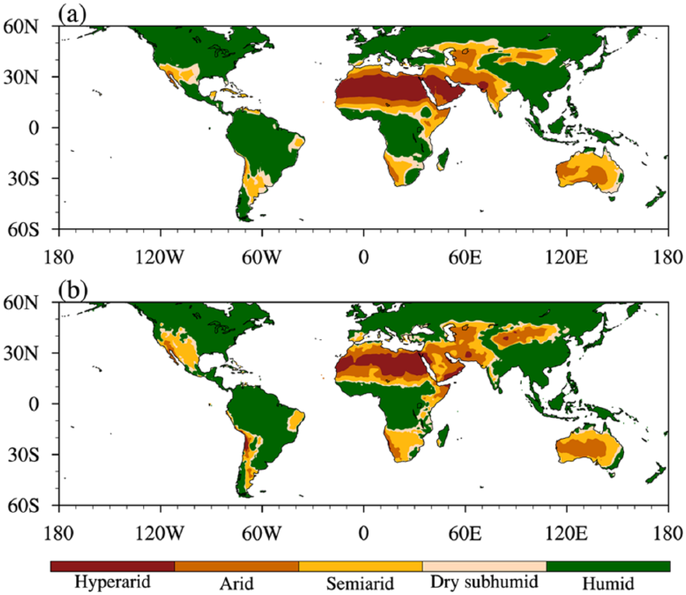
The climate classification based on AI of (a) the multi-model median field using data from the preindustrial control experiments and (b) the observation calculated using data from NCEP-2 (Kanamitsu et al., 2002) and PREC/L (Chen et al., 2002) in the period 1981–2010.

Spatial changes in drylands during the mid-Holocene

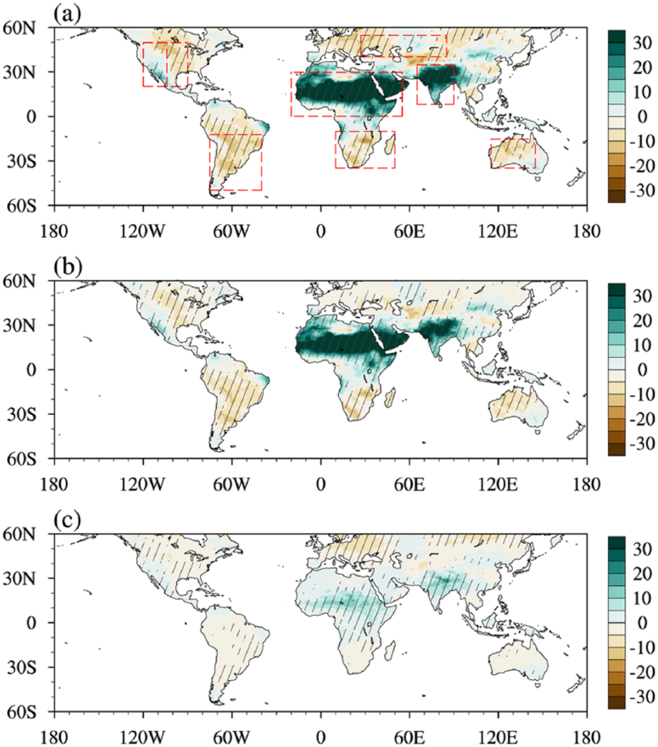
From the preindustrial period to the mid-Holocene, the area varies by –2% of the earth’s land surface for hyperarid zones and 1% for both arid and dry subhumid regions, indicating that there is little difference in the total area of drylands. Regarding transitions between varying climate subtypes, including the four types of drylands and the humid climate, 16% of preindustrial drylands convert to a wetter subtype, double the sum of zones that are replaced by a drier category. The dryland changes are not homogeneous across the globe (Figure 2). To be specific, a part of drylands disappears over northern Africa and northern India and forms newly over central North America, southern South America, southern Africa, and north of the Black Sea. Expansions of semiarid and dry subhumid climates occur in central North America, southern South America, southern Africa, eastern Europe, and central Asia, and expansions of the arid zones appear in Australia. Drylands contract and change to wetter climate categories across northern Africa and the Arabian Peninsula, with an average northward shift of 1.78° of the southern boundaries for all dryland subtypes in the region 0–30°N and 20°W–55°E; a similar wetter change also occurs in South Asia and southwestern North America.

Figure 2.

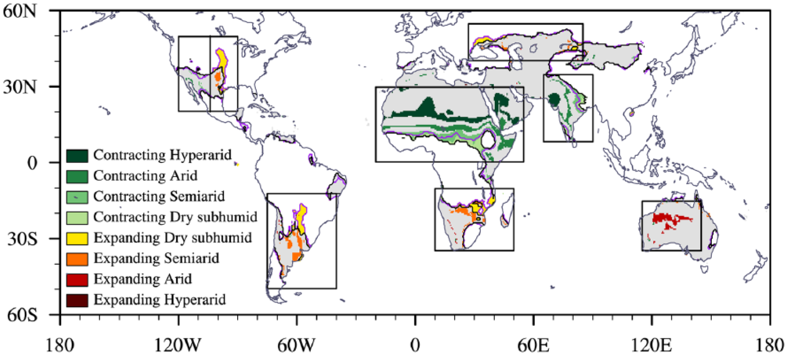
Mid-Holocene change in the dryland extent for the median field, depicted as stable (gray), contracting (green) and expanding (yellow to dark brown) zones. The spatial changes are plotted only where at least seven out of nine models agree on the sign of the median field change in the AI (Figure 3a). Dryland subtypes that convert into adjacent or nonadjacent wetter climate categories are labeled in figure using the word contracting, while subtypes that expand from wetter categories are labeled using expanding. More specifically, contractions of arid regions mean that the preindustrial arid climate converts into semiarid, dry subhumid or humid climates; expanding arid regions mean that the mid-Holocene arid climate is transited from preindustrial semiarid, dry subhumid or humid climates. Black and purple lines denote the dryland boundaries at the preindustrial period and mid-Holocene, respectively. Black boxes indicate eight focus regions, including three wetter regions (1) southwestern North America (referred to as SW N-America in the following figures), (2) northern Africa to the Arabian Peninsula (N Africa), and (3) South Asia (S Asia), and five drier regions (4) central North America (C N-America), (5) southern South America (S S-America), (6) southern Africa (S Africa), (7) eastern Europe to central Asia (Europe Asia), and (8) Australia.

In a further analysis at a regional scale, we specifically focus on eight regions, including three contracting (southwestern North America, northern Africa to the Arabian Peninsula, and South Asia) and five expanding zones (central North America, southern South America, southern Africa, eastern Europe to central Asia, and Australia). A criterion for the region selection is that at least five models agree on the subtype conversions shown in the median field (Figure 2). The areas of the regional dryland variations are specifically quantified (Figure 3). Because the net change in total drylands is small, the extent of total drylands (34% of the global land surface) is used as a common denominator to the absolute values of dryland changes for a convenient comparison. The newly formed dryland amounts to 2.2 × 10⁶ km² (4.3% of the global dryland area), with 25% of that area distributed in southern Africa, 16% in eastern Europe to central Asia, 21% in central North America, and 32% in southern South America. The overall loss of dryland area is 1.9 × 10⁶ km² (3.8% of the global dryland area), of which northern Africa to the Arabian Peninsula, South Asia, and southwestern North America account for 63%, 19%, and 5%, respectively. In addition, the northern Africa to the Arabian Peninsula region accounts for more than 60% of the contraction in every dryland subtype, and this region’s total contractions (12% of global drylands) are twofold larger than that of the rest regions (Figure 3c). Total expansions of individual dryland subtypes are equal to 8% of the global dryland area, 70% of which occur in southern continents (Figure 3d). Altogether, the multi-model median reveals the largest contraction of drylands from northern Africa to the Arabian Peninsula and a major expansion in the Southern Hemisphere.

Figure 3.

Area (10⁶ km²) of (a) drylands that are newly formed and disappeared, (b) expansions/contractions of individual types of drylands, and (c–d) total expansions/contractions of all subtypes of drylands for each region. Bars indicate the ensemble values as shown in Figure 2, and gray crosses mark values from individual models.

Toward more information on the consistency across models, we calculate the ratio of the inter-model spread to the absolute value of the multi-model median. Such ratios are 0.3–0.6 for contracting drylands, 0.4 for expanding ones in the total global land area and southern South America, but greater than 0.8 for other cases. In other words, the magnitudes of area changes are markedly consistent across individual models for such cases with small ratios, but vary largely for others.

Causes of dryland changes

Aridity changes

Relative to the preindustrial period, global drylands are 8% wetter as indicated by the decrease in AI (Figure 4a). Regionally, robust drying is found in most drylands except for the wetting found in southwestern North America and the northern Africa to South Asia zones, which is consistent with the aforementioned spatial changes in drylands. To investigate why the AI differs from that of the preindustrial period, we quantify the relative roles of precipitation (Figure 4b) and PET (Figure 4c) according to the approach proposed by Feng and Fu (2013), which can be written in the following form:

Δ A I \approx F (Δ P) + G (Δ P E T)

(4)

F (Δ P) = \frac{Δ P}{P E T}

(5)

G (Δ P E T) = - \frac{P}{P E T^{2}} Δ P E T + \frac{P}{P E T^{3}} {(Δ P E T)}^{2}

(6)

where $F (Δ P)$ and $G (Δ P E T)$ represent the respective contributions of precipitation and PET to AI changes, and ∆ ∆ $P,$ and ∆ $P E T$ indicate the changes in AI, precipitation (P), and PET, respectively. It is shown that the changes in precipitation and PET exert an influence in a same direction on AI. In other words, excessive precipitation and deficient PET favor wetness for drylands that become wetter, whereas deficient precipitation and excessive PET contribute to dryness in drier zones.

Figure 4.

Percentage changes of the median field between the mid-Holocene and the preindustrial period in (a) AI, which are caused by changes in (b) precipitation (hereafter referred to as P in figures) and (c) PET. Diagonal lines denote that at least seven out of nine models agree on the sign of the change.

Furthermore, a quantitative expression of regional precipitation and PET contributions is presented for their relative magnitudes (Figure 5). For contracting zones (Figure 5a), the multi-model medians of AI increase by 31%, 43%, and 44% for the global land, South Asia, and northern Africa to the Arabian Peninsula regions, respectively; more precipitation induces AI increases by 24%, 31%, and 34% in these regions, which is around twice larger than the PET effects. In southwestern North America, precipitation leads to an AI increase of 12% that is six times as many as PET does. For the expanding regions (Figure 5b), the AI is reduced by 9–16%, of which the precipitation deficit accounts for 80% for the global land, 89% for Australia, 77% for southern South America, 78% for central North America, 68% for eastern Europe to central Asia, and 90% for southern Africa. Altogether, precipitation contributes more than 68% of AI changes and is therefore a decisive factor for the mid-Holocene change in drylands.

Figure 5.

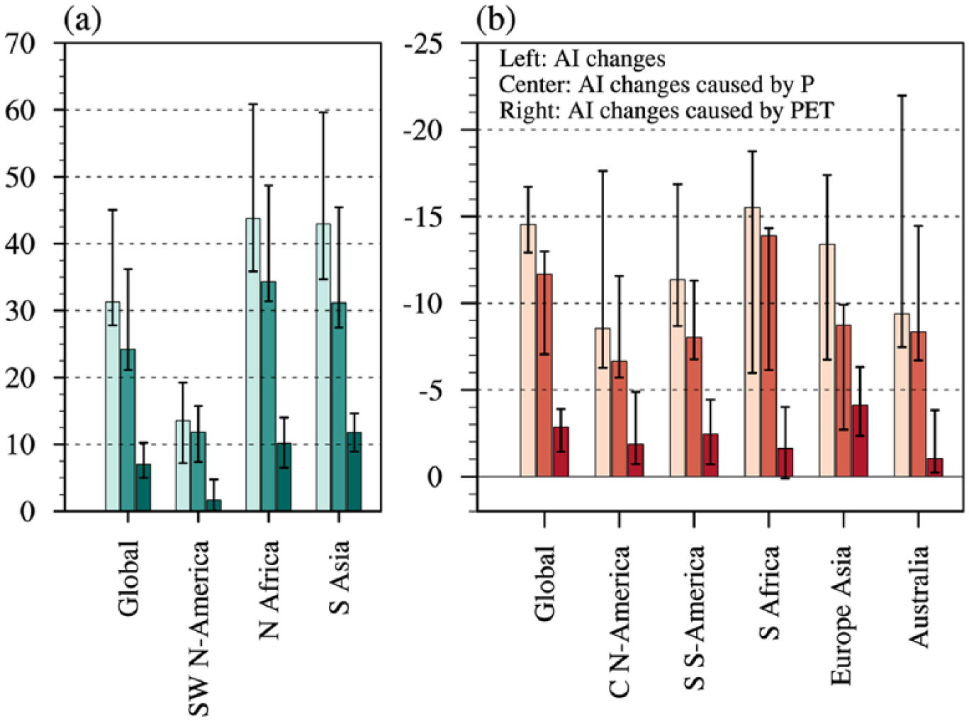
The regional average of AI changes (%) and the contributions of precipitation and PET for regions where drylands (a) contract and (b) expand. Colored bars indicate the multi-model medians, and error bars represent the interquartile ranges between individual simulations (25th and 75th percentiles).

Regarding the uncertainty in AI simulations, the ratios of inter-model spreads to multi-model medians are less than 0.6 for shrinking drylands from northern Africa to South Asia, as well as both types of changes on a global scale, indicating high agreement across models in the magnitude; for other cases, the ratios above 0.8 imply a certain uncertainty. Such ratios for AI changes are larger than those for precipitation contributions and are less than those for PET effects in almost all regions; specifically, the spreads between individual simulations of PET roles are larger than their median responses for southwestern North America and the five drier regions. Therefore, the uncertainties in PET are main sources that account for the difference between AI simulations.

Causes of PET changes

We decompose the PET anomalies into contributions of near-surface air temperature, AE, relative humidity, and wind speed (Figure 6) using the approach proposed by Fu and Feng (2014). For example, in order to derive the effect of the temperature change on PET, we calculate PET using temperature in the mid-Holocene but AE, relative humidity, and wind speed in the preindustrial period and use it to minus PET with all inputs from the preindustrial period. More details of isolating individual contributions are provided in the supplementary material. From northern Africa to South Asia, regional averages of 1.0°C cooling (Figure 6a) and 9–12% increases in relative humidity (Figure 6c) account for at least 30% and 50% of the PET decline, respectively. The main reasons for such increased relative humidity lie in the precipitation-induced tendency of more atmospheric water and the cooling-induced weakening of atmospheric moisture-holding ability. Inter-model spreads of temperature and relative humidity contributions are 0.2–0.8 times the magnitude of the median responses, indicating substantial consistency not only in the sign, but also in the magnitude across simulations. For southwestern North America, more than 80% of the PET decline comes from the contribution of a small increase in relative humidity (3%); however, its inter-model spread is nearly double the ensemble, and such a large scatter in the relative humidity contribution is the main reason for the uncertainty in PET reduction.

Figure 6.

PET changes (%) caused by changes in (a) near-surface air temperature (T_mean), (b) available energy (AE), (c) relative humidity (RH), and (d) wind speed (U₂). Diagonal lines denote that at least seven out of nine models agree on the sign of the change. The changes of T_mean indicate synchronous changes in both T_min and T_max.

For regions where drylands expand, only reduced relative humidity as influenced by precipitation deficit presents robust impacts (Figure 6c), which results in more than 60% of PET increases for most regions as expressed by the multi-model medians. However, the ratios of the interquartile ranges to ensembles are at least 1.5 on the regional scale, and such high uncertainties could translate into considerable model-to-model scatter in PET changes and further AI variations.

Altogether, the difference in relative humidity is the most important factor on PET changes with high consistency across models for regions with shrinking drylands and a certain uncertainty for regional expansions. Summarizing contributions from individual factors, including precipitation to AI changes (Figure 7), the median response suggests that precipitation and relative humidity collectively contribute 89% of AI variations for global shrinking drylands, 95% for global expanding ones, and 82–98% for individual regions, where precipitation roles are at least three times larger than that of relative humidity. The leading role of precipitation and secondary role of relative humidity are common characteristics to almost all models, although the simulated magnitudes vary from model to model.

Figure 7.

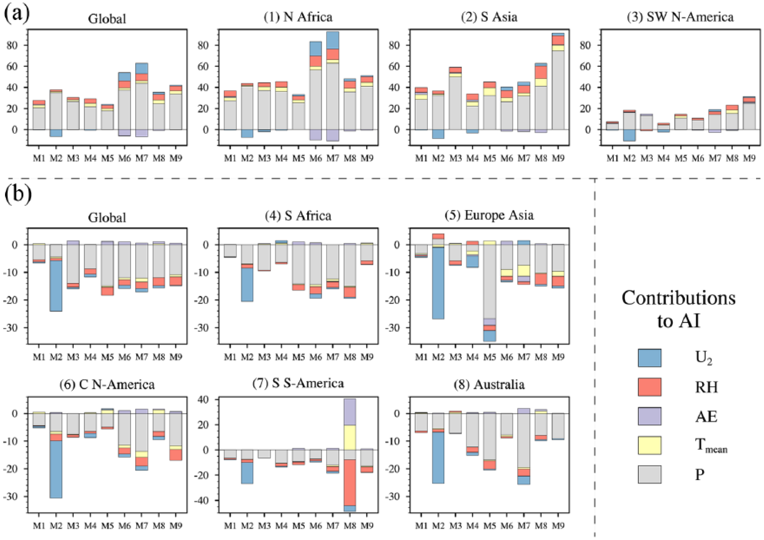
Regional averages of AI changes (%) caused by changes in precipitation (gray), T_mean (yellow), AE (purple), RH (red) and U₂ (blue) in regions of dryland (a) contractions (green zones in Figure 2) and (b) expansions (yellow to dark brown zones in Figure 2). The labels on x-axis denote the multi-model median (MM) and individual models (the serial numbers of models can be found in Table 1). Note the differences in y-axis ranges for wetter and drier transitions.

Aridity in paleo-data

Aridity changes are reflected primarily in vegetation taxa and lake levels, which are sensitive to two respective components of the water balance (Prentice et al., 1992b). Vegetation is sensitive to plant available moisture, that is, the necessary component of soil water that plants pull into their roots to sustain life during growing seasons. Such available moisture can be measured by an index alpha, defined by Prentice et al. (1992a) as a ratio of actual evapotranspiration to PET. In a catchment, water that is not evaporated or transpired accrues to runoff. Closed lakes tend toward an equilibrium level as a balance between runoff and the lake-surface water balance (Harrison et al., 1993), and this level is sensitive to changes in runoff (Prentice et al., 1992b). In addition, aridity changes can be indicated by other proxies, including sedimentology features, diatom abundances, dune activity, and stable isotopes. Given that paleo-data respond to diverse climate controls and have varying temporal resolutions, spatial coverages, and reconstruction methodologies, here we use multiple types of data to describe the past climate features, which are obtained from a synthesis of the present work for South America, South Asia, and Australia (Table S1 available online) and earlier compilations for other regions that have been published in peer-reviewed journals (Table 3).

Table 3.

Data complications regarding difference in moisture balance between the mid-Holocene and the present day.

Reference	Region	Record
Kohfeld and Harrison (2000) ^a	Global land	Lake level
Yu et al. (2001) ^a	Asia	Lake level
Harrison et al. (2003) ^a	North America	Lake level and geomorphic data
Liu et al. (2004)	Australia	Geomorphic and biological data
Ruter et al. (2004)	Northern tropical and subtropical Americas	Multiple proxies
Bartlein et al. (2011) ^b	Global land	Pollen
Chevalier et al. (2017)	Southern Africa	Multiple proxies

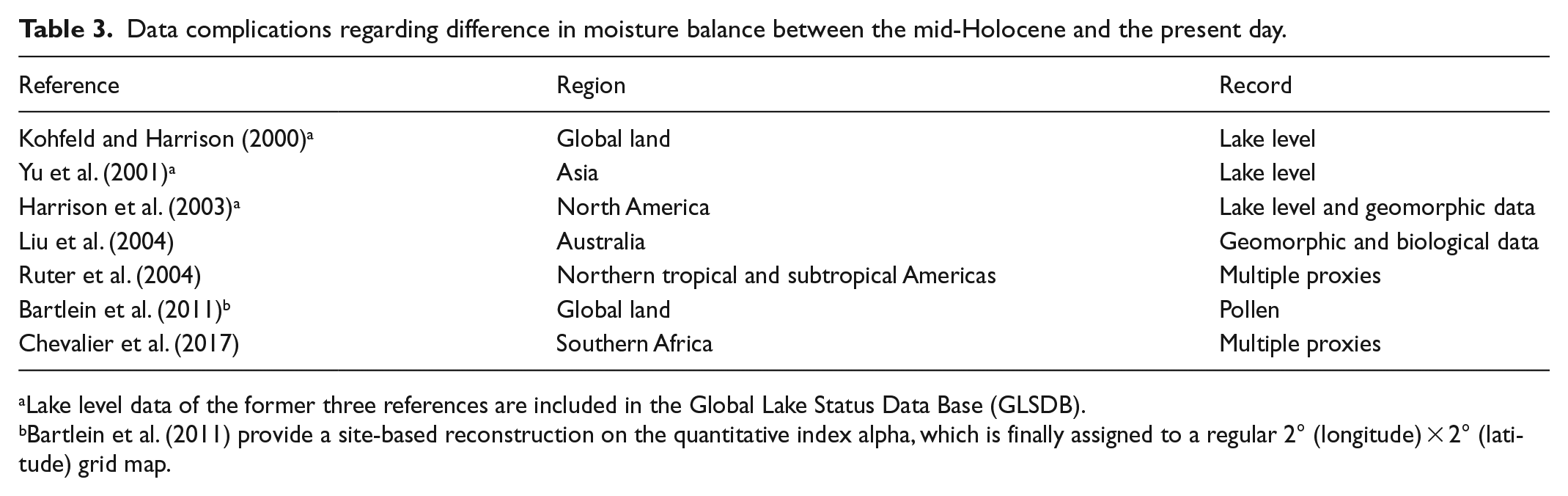
Lake level data of the former three references are included in the Global Lake Status Data Base (GLSDB).

Bartlein et al. (2011) provide a site-based reconstruction on the quantitative index alpha, which is finally assigned to a regular 2° (longitude) × 2° (latitude) grid map.

The comparison between the simulation (Figure 4a) and data (Figure 8) shows a broad consistency. Compared to the present day, wetter conditions are registered for all lake levels (Figure 8b) and most pollen records (Figure 8a) from northern Africa to the Arabian Peninsula, implying the existence of the Green Sahara during the mid-Holocene. Specifically, lakes and wetlands are estimated to have occupied 7% of the region 10–30°N and 17°W–60°E (Hoelzmann et al., 1998). Such wetter conditions agree with the simulation that produces a prominent shrink of drylands with an enormous aridity decline. Note that there is still a discrepancy in the extent of the wetness expansion, with proxy-inferred wetting located north of 15°N, but simulated wetting located further south (10–23°N). An evaluation of PMIP3 simulations (Perez-Sanz et al., 2014) indicates that the underestimate in the amount of precipitation change is at least 50% for 15–30°N Africa. For South Asia (Figure 8c), records for northern India reveal prevailing wetter conditions during the mid-Holocene (e.g. Dixit and Bera, 2011; Enzel et al., 1999; Singh et al., 1990). In western India, the presence of pollen belonging to evergreen taxa and the high phytolith climate index indicate a wetter-than-present Wadhwana (Prasad et al., 2014), whereas the luxuriant C₄ plants recorded by carbon isotope data reveal drier conditions in the adjacent Nal Sarovar (Prasad et al., 1997). Such a contradiction between pollen and carbon isotope data also appears across southern India (Rajagopalan et al., 1997; Vasanthy, 1988). In general, the simulation is able to reproduce the proxy-inferred decrease in aridity across the northern Indian subcontinent. For North America (Figure 8), alpha data (Bartlein et al., 2011), lake levels (Harrison et al., 2003), dune fields (Liu et al., 2004), and other proxies (Ruter et al., 2004) are mutually complementary. They collectively document wetter conditions from Mexico to the southwestern United States and drier conditions in the Great Plains from Canada to the United States, which is in congruence with the modeling. By contrast, there is no agreement reached in eastern North America where both simulations and paleo-records show uncertainties in the direction of moisture changes.

Figure 8.

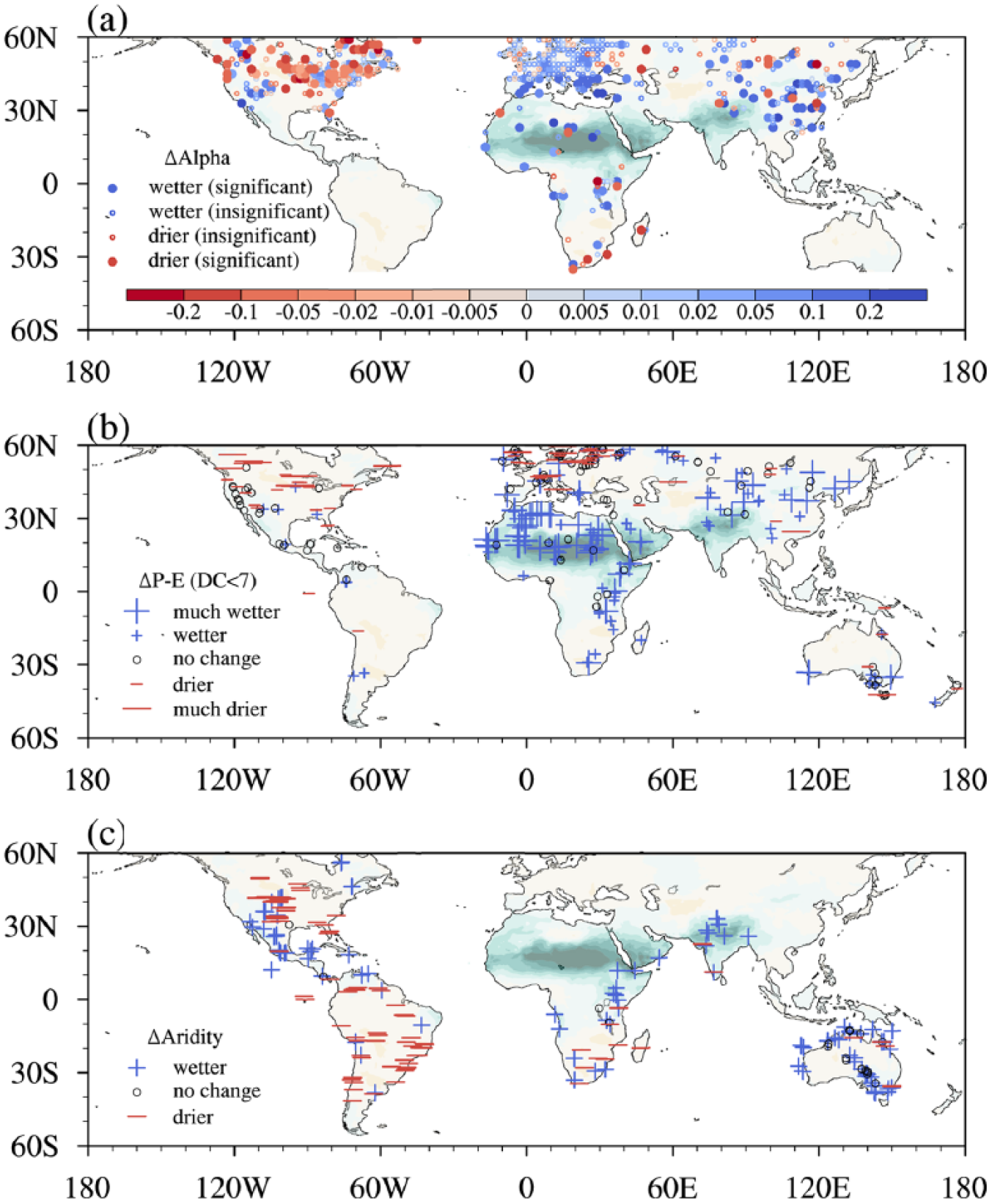
The mid-Holocene change relative to the present day in moisture inferred from (a) pollen records (Bartlein et al., 2011), (b) lake level data from GLSDB (Harrison et al., 2003; Kohfeld and Harrison, 2000; Yu et al., 2001), and (c) multiple proxies from other compilations (Chevalier et al., 2017; Harrison et al., 2003; Liu et al., 2004; Ruter et al., 2004) and the synthesis in this study (Table S1 available online). The background shading is the AI change. The bulk of the samples (79%) of pollen data in (a) fall within the period 5.5–6.5 cal. ka BP; 360 sites documenting lake levels from GLSDB are employed, while 18 poorly dated (Date Control = 7) sites are excluded.

Across South America (Figure 8c), we synthesize a diverse set of proxies for moisture variations (Table S1 available online), almost all of which document consistent directions to the modeling. For tropical zones, the climate change is characterized by wetting in the northernmost region (Venezuela) and drying to its south (the Amazonia and central to southern Brazil). Specifically, wetter Venezuela is registered in marine geochemical records (Haug et al., 2001) and lake sediment (Bradbury et al., 1981); in eastern Bolivia, pollen records reveal a shrinking Amazon rain forest during the mid-Holocene with the rain forest–savanna southern boundary retreating northward (Mayle et al., 2000); in eastern Amazonia and central to southern Brazil, dryness as indicated by a longer dry season or a shrinking of araucaria is registered in the data of charcoal sediments and pollen (e.g. Behling, 2002; Ledru, 1993; Turcq et al., 2002). In addition, desiccation is documented in most sites along the west coast, including Peru (Baker et al., 2001) and Chile (Jenny et al., 2002), and over southern zones of South America, including Uruguay (Iriarte, 2006) and western Argentina (Markgraf, 1987).

For Australia (Figure 8b and c), precipitation in northern zones is dominated by the Australian summer monsoon (ASM) in modern times. However, during the mid-Holocene, it is still a matter of debate whether the summer monsoon prevails (Markgraf et al., 1992; Wyrwoll and Miller, 2001) and whether it is weakened or strengthened in northern Australia (Beaufort et al., 2010; Jiang et al., 2015; Liu et al., 2004). Several paleo-data indicate a weaker-than-present ASM and a drier northern continent (Lough et al., 2014; Pickett et al., 2004). However, discordant with simulations, more records suggest a stronger-than-present ASM extended from northern Australia (Field et al., 2017; Haberle, 2005) into central Australia (Gliganic et al., 2014; Quigley et al., 2010). Such a stronger ASM has been interpreted as resulting from subdued ENSO activity with the prevalence of a La Niña-like mean state in the tropical Pacific (Gliganic et al., 2014; Quigley et al., 2010). The present climate of southern Australia is steered by the southern westerly winds. Over southeastern Australia, the mid-Holocene is marked by higher lake levels owing to the strengthening of westerlies (Fletcher and Moreno, 2012; Wilkins et al., 2013), whereas no robust signal is shown in the modeling there.

Along the west coast of Congo and Angola, data of both pollen (Dupont et al., 2008) and plant leaf wax (Schefuß et al., 2005) indicate a wetter condition, identical with the simulation. However, in the southern part of southern Africa, there are considerable uncertainties across proxies, including Madagascar. The proxies are quite limited over central Asia and it is therefore difficult to describe past features. For Europe, lake level records show disagreement in the sign, whereas pollen data register identically wetter conditions which differ from the simulation. Such a conflict is possibly attributed to PMIP3 models underestimating precipitation because of the inadequate simulation of westerly circulation and, thus, the moisture flux into the midcontinent (Bartlein et al., 2017; Mauri et al., 2014).

Discussion

Mechanisms behind precipitation change

Because the precipitation response to the mid-Holocene boundary conditions has been intensively investigated in earlier literature, we address the underlying mechanisms behind precipitation changes in regions of concern based on previous pertinent studies (e.g. Jiang et al., 2015; Liu et al., 2004; Zhao and Harrison, 2012). From northern Africa to South Asia, summer and autumn account for 60% and 40% of the increase in annual precipitation, respectively (Figure 9). In summer, the mid-Holocene orbital configuration induces more/less insolation and associated warming/cooling over northern/southern hemispheric land (Berger, 1978). Such a northern warming intensifies the summer monsoon (Bosmans et al., 2012; Jiang et al., 2015; Zhao and Harrison, 2012) by strengthening the land–sea contrast, deepening the thermal depression over land, and thus increasing moisture delivery from oceans into lands. Furthermore, one supplementary mechanism suggests that the regional wind–evaporation–sea surface temperature (SST) feedback in the Atlantic amplifies the orbitally increased precipitation over northern Africa, with a meridional SST contrast between the warming to the north of 5–10°N and the cooling to the south producing anomalous northward surface winds and consequent additional warming to the north (Braconnot et al., 2000; Zhao and Harrison, 2012; Zhao et al., 2005). In autumn, the simulated North Atlantic and Arabian Sea are warmer than today (Figure S2), which might be partly responsible for the excessive precipitation over land.

Figure 9.

The mid-Holocene change in precipitation (mm day⁻¹) for (a) December–February, (b) March–May, (c) June–August, and (d) September–November. Diagonal lines denote that at least seven out of nine models agree on the sign of the change.

For southern hemispheric drylands, summer as a primary contributor accounts for 41–89% of the annual precipitation deficit, and autumn contributes 35–60% (Figure 9). As an inverse of the response to direct orbital forcing in the Northern Hemisphere (Figure S3 available online), summer precipitation decreases in southern continents with a weakened continental thermal low, suppressed subtropical high, and coexistent reduction of moisture inflow (Bosmans et al., 2012; Jiang et al., 2015). Furthermore, the eastern boundary southerlies weaken as a feedback to the suppression of the oceanic subtropical high, which potentially reduces coastal upwelling activity and the northward advection of high-latitude cold water; such a process warms the ocean and increases coastal precipitation, to some extent mitigating the orbitally induced reduction in precipitation (e.g. Liu et al., 2004; Zhao and Harrison, 2012). In the present simulations, the orbital difference is the leading factor responsible for overall changes in precipitation rather than ocean feedbacks (Figure 9a), which agrees with the multi-model studies of Zhao and Harrison (2012) and Mantsis et al. (2013). However, a paradox occurs in northern Australia where Liu et al. (2004) and Marshall and Lynch (2006) highlight a more important impact of ocean feedbacks and thus an overall increase in precipitation based on a simulation using the Fast Ocean Atmosphere Model. In this regard, Zhao and Harrison (2012) have indicated that the result of only one model is possibly not as typical as that shown by multiple models. In autumn, the cooling sea surface (Figure S2 available online) is a potential reason for the precipitation decline, whereas the underlying mechanisms require a deeper analysis in the future.

For North America, pertinent studies have investigated the change in summer precipitation (Harrison et al., 2003; Zhao and Harrison, 2012). A northward shift of the Inter Tropical Convergence Zone (ITCZ) is found to intensify the summer monsoon across southwestern North America; the upward motion is accordingly enhanced across these monsoonal regions, leading to a compensatory subsidence anomaly and correspondingly less precipitation across adjacent central North America. In our analysis for the south-western zone, more than half of the annual precipitation increase occurs in spring rather than during summertime (Figure 9), and such a widespread increase in spring precipitation is common to all models. Based on a simulation using the NCAR Community Climate System Model, Diffenbaugh and Ashfaq (2007) reported a weaker California Current whose primary driver lies in variations of incoming solar energy. Likewise, our simulation shows a damped North Pacific subtropical high and accordingly suppressed eastern boundary wind stress (Figure S4 available online) in spring, which might weaken the coexistent cold current and thus favor more precipitation across southwestern North America. Such a weakened cold current is potentially supported by reduced offshore productivity in coastal northern California (Barron et al., 2003) and higher SST in the Santa Barbara Basin (Friddell et al., 2003).

Potential reasons for model–data discrepancy

Using diverse types of records, we show that the simulations and data are consistent in terms of the directions of AI changes for most regions. On the contrary, there is a certain model–data conflict in northern Africa and Australia, potential reasons for which are discussed below. In northern Africa, although the models produce a wetness expansion, they fail to produce as large an extent as that indicated by reconstructions. Such an underestimate might arise from the absence or poor treatment of indispensable processes such as vegetation (Harrison et al., 2015) and dust feedbacks (Pausata et al., 2016) in current models. Specifically, vegetation or soil is an important factor in land–air exchanges of water and energy; however, the debate has long prevailed as to whether the feedback is positive and which effect (surface albedo or evapotranspiration) is more important (Levis et al., 2004; Notaro et al., 2008; Wang et al., 2008) for northern Africa, which potentially implies the vegetation/soil–atmosphere interaction is not reasonably treated in the models considered here. Dust is reduced during the mid-Holocene Sahara because of increased rainfall, and a simulation using the EC-Earth model (version 3.1) reports that such a reduction could strengthen the vegetation–albedo feedback thus extending the northern monsoon limit approximately 500 km further (Pausata et al., 2016). However, the dust process has not been considered in all PMIP3 models.

In Australia, a conflict occurs between simulated drier conditions and reconstructed wetter ones from most records. In modern times, ENSO activity exerts strong impacts on the ASM, with El Niño conditions producing a weaker monsoon that results in aridity across the continental interior (Dai and Wigley, 2000). Based on a hypothesis that the modern ENSO–ASM relationship holds during the mid-Holocene, a number of reconstruction studies attribute the data-inferred wetness to an enhanced ASM because of the subdued ENSO activity that is characterized by infrequent or absent El Niño events (Gliganic et al., 2014; Quigley et al., 2010), which has been verified by records from both the eastern (e.g. Conroy et al., 2008; Keefer et al., 1998; Koutavas and Joanides, 2012) and western (e.g. Gagan et al., 2004; Tudhope et al., 2001) Pacific. However, PMIP3 models are unable to reproduce the magnitude of ENSO reduction as the proxy data suggest (Harrison et al., 2016; Tian et al., 2017), which might be partly responsible for the simulated opposite direction of aridity changes to reconstructions.

Conclusion

The dryland conditions during the mid-Holocene are investigated on the basis of the results of PMIP3 experiments undertaken by nine climate models. Compared to the preindustrial period, the total extent of drylands has changed less than 1%, global drylands are 8% wetter as indicated by an AI decline, and 16% of preindustrial drylands convert to a wetter climate subtype, double the sum of zones that are replaced by a drier category. Regionally, major contractions of each dryland subtype occur from northern Africa to the Arabian Peninsula, and their total extent is twofold larger than that of rest regions; arid, semiarid, and dry subhumid climates expand primarily in the Southern Hemisphere and second in central North America and eastern Europe to central Asia. The aforementioned changes are attributed first to differences in precipitation, whose contribution is at least four times the magnitude of the second factor, relative humidity. Their collective contributions equal 89% of the AI variations for global shrinking drylands, 95% for global expanding ones, and 82–98% for individual regions. The median response of simulations matches reasonably with proxy-based information on dryland aridity apart from some remarkable uncertainties across proxies for southern Africa and model–data discrepancies for Australia.

Supplemental Material

20190601-Supplementary_material-corrected – Supplemental material for Mid-Holocene drylands: A multi-model analysis using Paleoclimate Modelling Intercomparison Project Phase III (PMIP3) simulations

Supplemental material, 20190601-Supplementary_material-corrected for Mid-Holocene drylands: A multi-model analysis using Paleoclimate Modelling Intercomparison Project Phase III (PMIP3) simulations by Shanshan Liu, Dabang Jiang and Xianmei Lang in The Holocene

Footnotes

Acknowledgements

We acknowledge the NOAA/OAR/ESRL PSD for providing the reanalysis (National Centers for Environment Prediction – Department of Energy Atmospheric Model Intercomparison Project reanalysis (NCEP-2)) and observation (Precipitation Reconstruction over Land (PREC/L)) data and the climate modeling groups (listed in ) for producing and sharing their model outputs.

Funding

This work was supported by the National Natural Science Foundation of China (41625018), the National Key R&D Program of China (2017YFA0603404), and the National Natural Science Foundation of China (41421004).

Supplemental material

Supplemental material for this article is available online.

ORCID iD

Dabang Jiang

References

Allen

Pereira

Raes

, et al. (1998) Crop Evapotranspiration: Guidelines for Computing Crop Water Requirements (FAO Irrigation and Drainage Paper 56). Rome: Food and Agricultural Organization of the United Nations.

Baker

Seltzer

Fritz

, et al. (2001) The history of South American tropical precipitation for the past 25,000 years. Science 291: 640–643.

Barron

Heusser

Herbert

, et al. (2003) High-resolution climatic evolution of coastal northern California during the past 16,000 years. Paleoceanography 18: 1020.

Bartlein

Harrison

Izumi

(2017) Underlying causes of Eurasian midcontinental aridity in simulations of mid-Holocene climate. Geophysical Research Letters 44: 9020–9028.

Bartlein

Harrison

Brewer

, et al. (2011) Pollen-based continental climate reconstructions at 6 and 21 ka: A global synthesis. Climate Dynamics 37: 775–802.

Beaufort

van der Kaars

Bassinot

, et al. (2010) Past dynamics of the Australian monsoon: Precession, phase and links to the global monsoon concept. Climate of the Past 6: 695–706.

Behling

(2002) South and southeast Brazilian grasslands during late quaternary times: A synthesis. Palaeogeography, Palaeoclimatology, Palaeoecology 177: 19–27.

Berger

(1978) Long-term variations of daily insolation and quaternary climatic changes. Journal of the Atmospheric Sciences 35: 2362–2367.

Bosmans

JHC

Drijfhout

Tuenter

, et al. (2012) Monsoonal response to mid-Holocene orbital forcing in a high resolution GCM. Climate of the Past 8: 723–740.

10.

Braconnot

Harrison

Kageyama

, et al. (2012) Evaluation of climate models using palaeoclimatic data. Nature Climate Change 2: 417–424.

11.

Braconnot

Marti

Joussaume

, et al. (2000) Ocean feedback in response to 6 kyr BP insolation. Journal of Climate 13: 1537–1553.

12.

Bradbury

Leyden

Salgado-Labouriau

, et al. (1981) Late quaternary environmental history of lake Valencia, Venezuela. Science 214: 1299–1305.

13.

Chen

Xie

Janowiak

, et al. (2002) Global land precipitation: A 50-year monthly analysis based on gauge observations. Journal of Hydrometeorology 3: 249–266.

14.

Chevalier

Brewer

Chase

(2017) Qualitative assessment of PMIP3 rainfall simulations across the eastern African monsoon domains during the mid-Holocene and the last glacial maximum. Quaternary Science Reviews 156: 107–120.

15.

Conroy

Overpeck

Cole

, et al. (2008) Holocene changes in eastern tropical Pacific climate inferred from a Galápagos lake sediment record. Quaternary Science Reviews 27: 1166–1180.

16.

Dai

Wigley

TML

(2000) Global patterns of ENSO-induced precipitation. Geophysical Research Letters 27: 1283–1286.

17.

Diffenbaugh

Ashfaq

(2007) Response of California current forcing to mid-Holocene insolation and sea surface temperatures. Paleoceanography 22: PA3101.

18.

Dixit

Bera

(2011) Mid-Holocene vegetation and climatic variability in tropical deciduous sal (Shorea robusta) forest of lower Brahmaputra valley, Assam. Journal of the Geological Society of India 77: 419–432.

19.

Dupont

Behling

Kim

(2008) Thirty thousand years of vegetation development and climate change in Angola (Ocean Drilling Program Site 1078). Climate of the Past 4: 107–124.

20.

Enzel

Ely

Mishra

, et al. (1999) High-resolution Holocene environmental changes in the Thar desert, northwestern India. Science 284: 125–128.

21.

Feng

(2013) Expansion of global drylands under a warming climate. Atmospheric Chemistry and Physics 13: 10081–10094.

22.

Field

McGowan

Moss

, et al. (2017) A late quaternary record of monsoon variability in the northwest Kimberley, Australia. Quaternary International 449: 119–135.

23.

Fletcher

M-S

Moreno

(2012) Have the southern westerlies changed in a zonally symmetric manner over the last 14,000 years? A hemisphere-wide take on a controversial problem. Quaternary International 253: 32–46.

24.

Friddell

Thunell

Guilderson

, et al. (2003) Increased northeast Pacific climatic variability during the warm middle Holocene. Geophysical Research Letters 30: 1560.

25.

Feng

(2014) Responses of terrestrial aridity to global warming. Journal of Geophysical Research: Atmospheres 119: 7863–7875.

26.

Gagan

Hendy

Haberle

, et al. (2004) Post-glacial evolution of the Indo-Pacific warm pool and El Niño-Southern oscillation. Quaternary International 118–119: 127–143.

27.

Gaur

Squires

(2018) Geographic extent and characteristics of the world’s arid zones and their peoples. In: Gaur

Squires

(eds) Climate Variability Impacts on Land Use and Livelihoods in Drylands. Cham: Springer, pp. 3–20.

28.

Gleckler

Taylor

Doutriaux

(2008) Performance metrics for climate models. Journal of Geophysical Research: Atmospheres 113: D06104.

29.

Gliganic

Cohen

May

J-H

, et al. (2014) Late-Holocene climatic variability indicated by three natural archives in arid southern Australia. The Holocene 24: 104–117.

30.

Haberle

(2005) A 23,000-yr pollen record from Lake Euramoo, wet tropics of NE Queensland, Australia. Quaternary Research 64: 343–356.

31.

Harrison

Bartlein

Prentice

(2016) What have we learnt from palaeoclimate simulations? Journal of Quaternary Science 31: 363–385.

32.

Harrison

Bartlein

Izumi

, et al. (2015) Evaluation of CMIP5 palaeo-simulations to improve climate projections. Nature Climate Change 5: 735–743.

33.

Harrison

Kutzbach

Liu

, et al. (2003) Mid-Holocene climates of the Americas: A dynamical response to changed seasonality. Climate Dynamics 20: 663–688.

34.

Harrison

Prentice

Guiot

(1993) Climatic controls on Holocene lake-level changes in Europe. Climate Dynamics 8: 189–200.

35.

Haug

Hughen

Sigman

, et al. (2001) Southward migration of the intertropical convergence zone through the Holocene. Science 293: 1304–1308.

36.

Hobbins

Wood

Mcevoy

, et al. (2016) The evaporative demand drought index – Part I: Linking drought evolution to variations in evaporative demand. Journal of Hydrometeorology 17: 1745–1761.

37.

Hoelzmann

Jolly

Harrison

, et al. (1998) Mid-Holocene land-surface conditions in northern Africa and the Arabian Peninsula: A data set for the analysis of biogeophysical feedbacks in the climate system. Global Biogeochemical Cycles 12: 35–51.

38.

Huang

Xie

, et al. (2016a) Global semi-arid climate change over last 60 years. Climate Dynamics 46: 1131–1150.

39.

Huang

Guan

, et al. (2016b) Accelerated dryland expansion under climate change. Nature Climate Change 6: 166–172.

40.

Iriarte

(2006) Vegetation and climate change since 14,810 14C yr B.P. in southeastern Uruguay and implications for the rise of early formative societies. Quaternary Research 65: 20–32.

41.

Jenny

Valero-Garcés

Villa-Martínez

, et al. (2002) Early to mid-Holocene aridity in central Chile and the southern westerlies: The Laguna Aculeo record (34°S). Quaternary Research 58: 160–170.

42.

Jiang

Tian

Lang

(2013) Mid-Holocene net precipitation changes over China: Model–data comparison. Quaternary Science Reviews 82: 104–120.

43.

Jiang

Tian

Lang

(2015) Mid-Holocene global monsoon area and precipitation from PMIP simulations. Climate Dynamics 44: 2493–2512.

44.

Kanamitsu

Ebisuzaki

Woollen

, et al. (2002) NCEP–DOE AMIP-II reanalysis (R-2). Bulletin of the American Meteorological Society 83: 1631–1643.

45.

Keefer

deFrance

Moseley

, et al. (1998) Early maritime economy and El Niño events at Quebrada Tacahuay, Peru. Science 281: 1833–1835.

46.

Kohfeld

Harrison

(2000) How well can we simulate past climates? Evaluating the models using global palaeoenvironmental datasets. Quaternary Science Reviews 19: 321–346.

47.

Koutavas

Joanides

(2012) El Niño – Southern Oscillation extrema in the Holocene and last glacial maximum. Paleoceanography 27: PA4208.

48.

Ledru

M-P

(1993) Late quaternary environmental and climatic changes in central Brazil. Quaternary Research 39: 90–98.

49.

Levis

Bonan

Bonfils

(2004) Soil feedback drives the mid-Holocene North African monsoon northward in fully coupled CCSM2 simulations with a dynamic vegetation model. Climate Dynamics 23: 791–802.

50.

Liu

Harrison

Kutzbach

, et al. (2004) Global monsoons in the mid-Holocene and oceanic feedback. Climate Dynamics 22: 157–182.

51.

Lough

Llewellyn

Lewis

, et al. (2014) Evidence for suppressed mid-Holocene northeastern Australian monsoon variability from coral luminescence. Paleoceanography 29: 581–594.

52.

Mantsis

Lintner

Broccoli

, et al. (2013) Mechanisms of mid-Holocene precipitation change in the south Pacific convergence zone. Journal of Climate 26: 6937–6953.

53.

Markgraf

(1987) Paleoenvironmental changes at the northern limit of the subantarctic Nothofagus forest, lat 37°S, Argentina. Quaternary Research 28: 119–129.

54.

Markgraf

Dodson

Kershaw

, et al. (1992) Evolution of late Pleistocene and Holocene climates in the circum-south Pacific land areas. Climate Dynamics 6: 193–211.

55.

Marshall

Lynch

(2006) Time-slice analysis of the Australian summer monsoon during the late quaternary using the Fast Ocean Atmosphere Model. Journal of Quaternary Science 21: 789–801.

56.

Marzin

Braconnot

(2009) The role of the ocean feedback on Asian and African monsoon variations at 6 kyr and 9.5 kyr BP. Comptes Rendus Geoscience 341: 643–655.

57.

Mauri

Davis

BAS

Collins

, et al. (2014) The influence of atmospheric circulation on the mid-Holocene climate of Europe: A data-model comparison. Climate of the Past 10: 1925–1938.

58.

Mayle

Burbridge

Killeen

(2000) Millennial-scale dynamics of southern Amazonian rain forests. Science 290: 2291–2294.

59.

Middleton

Thomas

DSG

(1997) World Atlas of Desertification. 2nd Edition. London: Arnold – A Member of the Hodder Headline Group.

60.

Notaro

Wang

Liu

, et al. (2008) Combined statistical and dynamical assessment of simulated vegetation-rainfall interactions in North Africa during the mid-Holocene. Global Change Biology 14: 347–368.

61.

Pausata

FSR

Messori

Zhang

(2016) Impacts of dust reduction on the northward expansion of the African monsoon during the Green Sahara period. Earth and Planetary Science Letters 434: 298–307.

62.

Perez-Sanz

González-Sampériz

, et al. (2014) Evaluation of modern and mid-Holocene seasonal precipitation of the Mediterranean and northern Africa in the CMIP5 simulations. Climate of the Past 10: 551–568.

63.

Pickett

Harrison

Hope

, et al. (2004) Pollen-based reconstructions of biome distributions for Australia, Southeast Asia and the Pacific (SEAPAC region) at 0, 6000 and 18,000 14C yr BP. Journal of Biogeography 31: 1381–1444.

64.

Prasad

Kusumgar

Gupta

(1997) A mid to late-Holocene record of palaeoclimatic changes from Nal Sarovar: A palaeodesert margin lake in western India. Journal of Quaternary Science 12: 153–159.

65.

Prasad

Farooqui

Sharma

, et al. (2014) Mid-late Holocene monsoonal variations from mainland Gujarat, India: A multi-proxy study for evaluating climate culture relationship. Palaeogeography, Palaeoclimatology, Palaeoecology 397: 38–51.

66.

Prentice

Cramer

Harrison

, et al. (1992a) A global biome model based on plant physiology and dominance, soil properties and climate. Journal of Biogeography 19: 117–134.

67.

Prentice

Guiot

Harrison

(1992b) Mediterranean vegetation, lake levels and palaeoclimate at the last glacial maximum. Nature 360: 658–660.

68.

Quigley

Horton

Hellstrom

, et al. (2010) Holocene climate change in arid Australia from speleothem and alluvial records. The Holocene 20: 1093–1104.

69.

Rajagopalan

Sukumar

Ramesh

, et al. (1997) Late quaternary vegetational and climatic changes from tropical peats in southern India – An extended record up to 40,000 years BP. Current Science 73: 60–63.

70.

Ruter

Arzt

Vavrus

, et al. (2004) Climate and environment of the subtropical and tropical Americas (NH) in the mid-Holocene: Comparison of observations with climate model simulations. Quaternary Science Reviews 23: 663–679.

71.

Safriel

Adeel

Niemeijer

, et al. (2005) Dryland systems. In: Hassan

Scholes

Ash

(eds) Millennium Ecosystem Assessment – Ecosystems and Human Well-Being: Current State and Trends. Volume 1. Washington, DC: World Resources Institute, pp. 623–662.

72.

Scheff

(2019) A unified wetting and drying theory. Nature Climate Change 9: 9–10.

73.

Schefuß

Schouten

Schneider

(2005) Climatic controls on central African hydrology during the past 20,000 years. Nature 437: 1003–1006.

74.

Sidahmed

(2018) Recent trends in drylands and future scope for advancement. In: Gaur

Squires

(eds) Climate Variability Impacts on Land Use and Livelihoods in Drylands. Cham: Springer, pp. 21–57.

75.

Singh

Wasson

Agrawal

(1990) Vegetational and seasonal climatic changes since the last full glacial in the Thar desert, northwestern India. Review of Palaeobotany and Palynology 64: 351–358.

76.

Taylor

(2001) Summarizing multiple aspects of model performance in a single diagram. Journal of Geophysical Research: Atmospheres 106: 7183–7192.

77.

Tian

Jiang

, et al. (2017) Causes of ENSO weakening during the mid-Holocene. Journal of Climate 30: 7049–7070.

78.

Tudhope

Chilcott

McCulloch

, et al. (2001) Variability in the El Niño-Southern Oscillation through a glacial-interglacial cycle. Science 291: 1511–1517.

79.

Turcq

Albuquerque

ALS

Cordeiro

, et al. (2002) Accumulation of organic carbon in five Brazilian lakes during the Holocene. Sedimentary Geology 148: 319–342.

80.

United Nations Educational, Scientific and Cultural Organization (1979) Map of the World Distribution of Arid Regions: Explanatory Note (MAB Technical Notes 7). Paris: The United Nations Educational, Scientific and Cultural Organization.

81.

Vasanthy

(1988) Pollen analysis of late quaternary sediments: Evolution of upland Savanna in Sandynallah (Nilgiris, south India). Review of Palaeobotany and Palynology 55: 175–192.

82.

Wang

Notaro

Liu

, et al. (2008) Detecting vegetation-precipitation feedbacks in mid-Holocene north Africa from two climate models. Climate of the Past 4: 59–67.

83.

Wilkins

Gouramanis

De Deckker

, et al. (2013) Holocene lake-level fluctuations in Lakes Keilambete and Gnotuk, southwestern Victoria, Australia. The Holocene 23: 784–795.

84.

Wyrwoll

K-H

Miller

(2001) Initiation of the Australian summer monsoon 14,000 years ago. Quaternary International 83–85: 119–128.

85.

Yang

Roderick

Zhang

, et al. (2019) Hydrologic implications of vegetation response to elevated CO2 in climate projections. Nature Climate Change 9: 44–48.

86.

Chen

, et al. (2000) Palaeovegetation of China: A pollen data-based synthesis for the mid-Holocene and last glacial maximum. Journal of Biogeography 27: 635–664.

87.

Harrison

Xue

(2001) Lake Status Records from China: Data Base Documentation. Technical Report. Jena: Max-Planck-Institut für Biogeochemie.

88.

Zhao

Harrison

(2012) Mid-Holocene monsoons: A multi-model analysis of the inter-hemispheric differences in the responses to orbital forcing and ocean feedbacks. Climate Dynamics 39: 1457–1487.

89.

Zhao

Braconnot

Marti

, et al. (2005) A multi-model analysis of the role of the ocean on the African and Indian monsoon during the mid-Holocene. Climate Dynamics 25: 777–800.

Supplementary Material

Please find the following supplemental material available below.

For Open Access articles published under a Creative Commons License, all supplemental material carries the same license as the article it is associated with.

For non-Open Access articles published, all supplemental material carries a non-exclusive license, and permission requests for re-use of supplemental material or any part of supplemental material shall be sent directly to the copyright owner as specified in the copyright notice associated with the article.

0.00 MB

1.65 MB