Late-Holocene climate response and glacial fluctuations revealed by the sediment record of the monsoon-dominated Chorabari Lake,Central Himalaya

Abstract

We studied a periglacial lake situated in the monsoon-dominated Central Himalaya where an interplay of monsoonal precipitation and glacial fluctuations during the late Holocene is well preserved. A major catastrophe occurred on 16–17 June 2013, with heavy rains causing rupturing of the moraine-dammed Chorabari Lake located in the Mandakini basin, Central Himalaya, and exposed 8-m-thick section of the lacustrine strata. We reconstructed the late-Holocene climatic variability in the region using multi-parametric approach including magnetic, mineralogical and chemical (XRF) properties of sediments, paired with grain size and optically simulated luminescence (OSL) dating. The OSL chronology suggests that the lake was formed by a lateral moraine during the deglaciation phase of Chorabari Glacier between 4.2 and 3.9 ka and thereafter the lake deposited about 8-m-thick sediment sequence in the past 2.3 ka. The climatic reconstruction of the lake broadly represents the late-Holocene glacial chronology of the Central Himalaya coupled with many short-term climatic perturbations recorded at a peri-glacial lake setting. The major climatic phases inferred from the study suggests (1) a cold period between 260 BCE and 270 CE, (2) warmer conditions between 900 and 1260 CE for glacial recession and (3) glacial conditions between ~1370 and 1720 CE when the glacier gained volume probably during the ‘Little Ice Age’ (LIA). We suggest a high glacial sensitivity to climatic variability in the monsoon-dominated region of the Himalaya.

Keywords

Chorabari Lake glacial variability Himalaya late-Holocene climate

Introduction

Glacial lakes are one of the best proxy indicators of climatic perturbations. In the short term, the accumulated snow/ice melt produced in response to warming serves as a driving mechanism to preserve the climatic signals in the form of annual layers at lake archives, whereas dynamics of glaciers related to long-term climatic stability reflects in the form of massive landforms, i.e., moraines. The quality and replication of the glacial fluctuations, particularly for the moraine deposits during the Holocene epoch, have improved dramatically in the recent decades (Bisht et al., 2015; Murari et al., 2014; Owen and Dortch, 2014; Shukla et al., 2018). The chronological correlations based on the age range of two glacial events with one or two standard deviations led us to believe that the high-resolution climatic events captured by periglacial lake might be of particular importance to study glaciation/deglaciation pattern in the Himalaya as related to climatic changes.

The Himalayan system is divisible into two most important climatic components, that is, the Indian Summer Monsoon (ISM) and the Mid-Latitude Westerlies (MLW). The ISM delivers considerable amount of precipitation during summer months via northward migration of the Inter Tropical Convergence Zone (ITCZ; Chao and Chen, 2001; Gadgil et al., 2003; Yancheva et al., 2007), whereas the MLW bring moisture from the Mediterranean, Black and Caspian seas and deliver over the northwestern (NW) Himalaya in summer and in the NW and Central Himalaya during winter months (Figure 1). The precipitation and basin runoff generally decrease from the east to the west owing to weakening of the ISM trough as it moves westward along the Himalayan range (Bookhagen and Burbank, 2010). The ISM precipitation dominates in the eastern Himalaya, while in the west, westerly circulation and cyclonic storms (MLW) contribute about two-thirds of the annual precipitation in the form of high-altitude snowfall during winter, with the remaining one-third resulting from summer precipitation mainly because of monsoon circulation (Armstrong, 2010; Wake, 1989). These complex weather systems make difficult to understand the climate processes in the Himalaya. A recent study from the Kedarnath area, Mandakini Valley, Central Himalaya, suggested that the Chorabari Lake offers an excellent ambience for preservation of such palaeo-records (Srivastava et al., 2017). Numerous high-resolution palaeo-records of the Himalaya suggest that the temperature and precipitation conditions of the Himalaya are strongly controlled by variations in insolation on orbital and decadal time scales (Gupta et al., 2003, 2005; Shukla et al., 2018).

Figure 1.

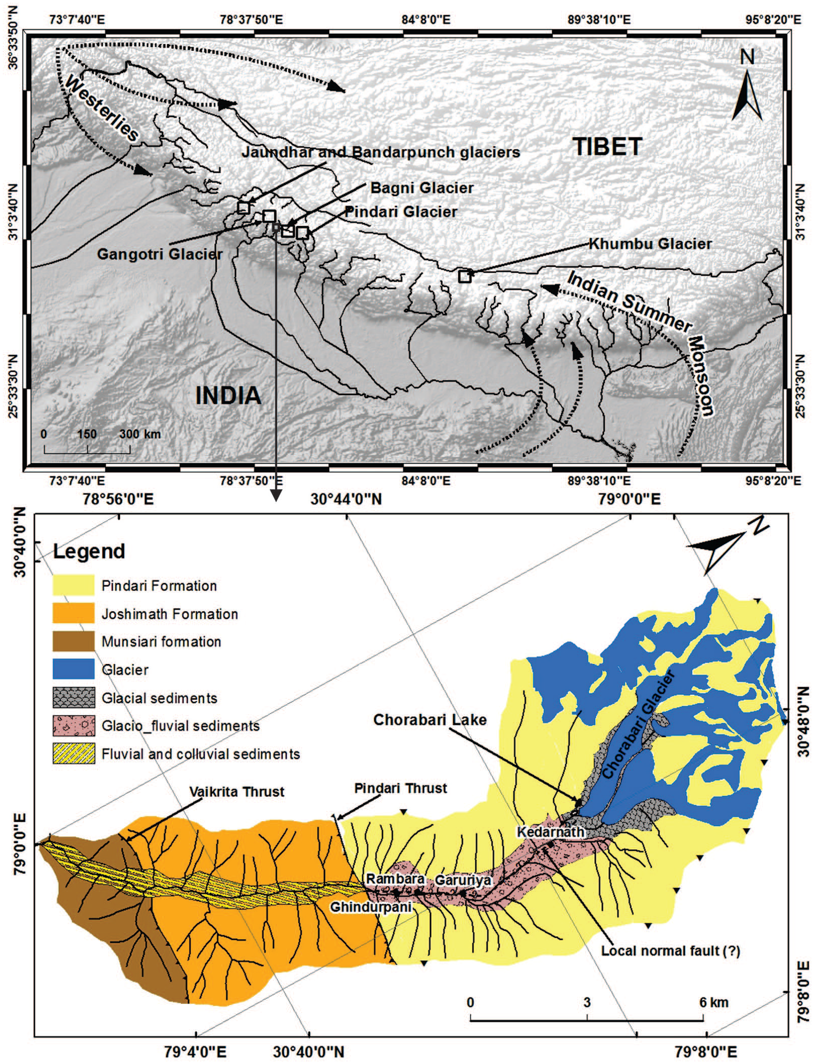
The Shuttle Radar Topography Mission (SRTM) image showing the location of Mandakini basin (Chorabari Lake) and adjacent glacier valleys of the Himalaya, which are mainly under the influence of the Indian Summer Monsoon and Mid-Latitude Westerlies (top). Detailed geological and geomorphological characteristics of the Chorabari Glacier; dark-shaded areas indicate glacier boundaries (bottom).

The present study attempts to document high-resolution changes in sediment deposition patterns in a high glacial lake environment. This is of particular importance to understand the role of climate in driving the glaciation in a monsoon-dominated glacierized basin of the Himalaya. The main objective is to understand the diverse role of complexities in the glacial-climate system by reconstructing the late-Holocene climate variations using the glacial lake sediment records from the Mandakini River Basin, Central Himalaya, India.

Site description

The Mandakini River Basin lies at a latitude of 30°15°N to 30°45′N and longitude of 78°48′E to 79°20′E comprising an catchment area of 2250 km². The valley has a complex topography comprising high mountain ranges with a glaciated basin in the north and fluvial terraces in the central and lower parts. Lying between 640 and 6940 m a.s.l., the valley is dotted with several high peaks like Bharat Khunta (6578 m a.s.l.), Kedarnath peak (6940 m a.s.l.), Mahalaya peak (5970 m a.s.l.) and Hanuman top (5320 m a.s.l.). The Chorabari (6.6 km²) and Companion (2.5 km²) glaciers are the two largest glaciers in the valley alongside a few other small glaciers including ice apron, hanging glaciers, glacierete and cirque glaciers (Figure 1). The area has two high-altitude lakes that are directly fed by snow/ice melt, avalanches and rain water. The moraine-dammed Chorabari Lake is situated on the right flank of the Chorabari Glacier (Figure 1), is ~300 m long, and is ~175 m wide, with a maximum depth of 30 m covering an area of 3.6 × 10⁴ m² (Bhambri et al., 2016; Mehta et al., 2017). Prior to the breaching on 16–17 June 2013 rain event, the mean water level of the lake was 19 m (Mehta et al., 2017). The lake had no outlets, and the water is simply released through narrow passages (seepage) at the base of the lake (Figure 2). However, recent lake history suggests that between the years 2003 and 2012, the lake was completely dry in the months of June and October/November but partially filled (~5 m based on field observations) during the rainy season (July, August and September). In winter months, the lake remained fully covered by snow and avalanches (Figure 2).

Figure 2.

Photograph showing the downstream view of Chorabari Lake in different seasons, i.e. (a) snow- and avalanche-filled lake, (b) dry lake, (c) partially filled lake and (d) after breached lake. The maximum height of lake (30 m) from the top of the moraine ridge is presented in panel (b) and the height of exposed stratigraphy (8 m) is presented in panel (d).

Heavy rain on 16–17 June 2013 triggered the rupture of the moraine-dammed Chorabari Lake that caused massive outpouring of the Mandakini River (Dobhal et al., 2013b). The lake burst released an estimated ~0.68 × 10⁶ m³ volume of water, sweeping away ~0.13 × 10⁶ m³ of lake sediment by volume (Mehta et al., 2017). As a result, about ~8-m-thick section of lake sediment (sand/silt/clay; commonly 0.12–69 cm thick) was exposed. Geologically, the area falls in the Pindari Formation of the Precambrian Vaikrita Group, composed of highly metamorphosed banded calc-silicate gneiss, calc-schist, biotite psammitic gneiss, pegmatite, granite, porphyroblastic augen gneiss and so on (Valdiya et al., 1999; Figure 1).

Modern climate

The general climate of the study area is warm-humid in summer and dry-cold in winter (Dobhal et al., 2013a). The area receives heavy ISM precipitation during the summer and maximum snowfall in winter from December to March mostly from MLW (Dobhal et al., 2013a; Mehta et al., 2012; Owen et al., 1996). The monitoring of the Chorabari Glacier by the scientists of the Wadia Institute of Himalayan Geology began in 2003 and a conventional meteorological station was established near the snout to collect the data on air temperature, wind speed and precipitation (Dobhal et al., 2013a). In 2007, an automatic weather station (Campbell Instrument) was installed near the snout of the glacier at an altitude of 3820 m a.s.l. Air temperature, solar radiation, sunshine duration, wind speed and precipitation have been continuously monitored since then. The summer (June–October) mean temperature fluctuates between +3°C and +12°C during the period 2007–2012 (Mehta et al., 2014). The maximum air temperature recorded was 16.7°C in June 2012 and the minimum was −19.5°C in February 2012. The average wind speed was 2.5 m/s and the average daily sunshine duration was 190 min/day. The winter snow depth was measured between 25 and 50 cm in the month of April and early May during 2007–2012 which melted before the commencement of the summer monsoon in mid-June (Dobhal et al., 2013b; Mehta et al., 2017).

Mehta et al. (2017) analysed the rainfall data from the India Meteorological Department (IMD), India Water Portal and Tropical Rainfall Measuring Mission (TRMM). More than 100 years (1901–2013) of data from the Bhagirathi basin, Uttarkashi, suggests that extreme rainfall events have increased abruptly since the year 2000 (Figure 3). The plot of temperature and precipitation anomalies shows that the temperatures are increasing continuously after 1990, while precipitation frequency makes sharp upward trend after the year 2000 (Mehta et al., 2017).

Figure 3.

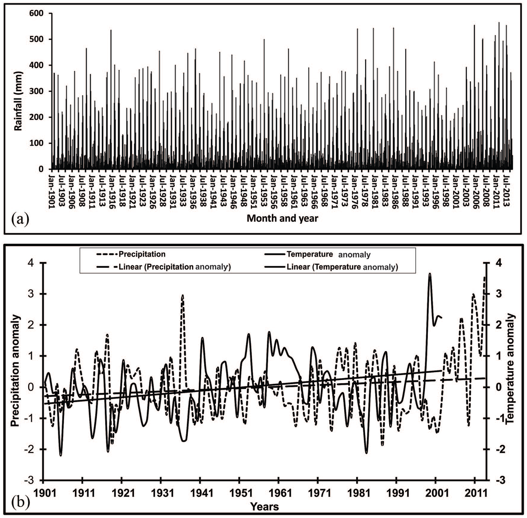
Rainfall and temperature distribution in Uttarkashi (N30°43′47″; E78°26′39″). (a) The bar diagram shows >100 years (1901–2013) of rainfall in Uttarkashi (IMD and TRMM data). (b) The line diagram shows temperature (1901–2001) and rainfall (1901–2013) anomalies. The trend line of figure depicts the temperature and precipitation increasing trends. The figure also shows that the temperature and precipitation sharply increased after AD 1990 and AD 2000, respectively (after Mehta et al., 2017; data taken from IMD and TRMM).

Materials and methods

Sediment stratigraphy

After breaching of the Chorabari Lake, a thick section of sediments was exposed. We selected the section having a maximum exposed thickness of ~8 m section (Figures 2 and 4) for sampling. The sampled section is composed of mixed size sediment consisting of coarser sand, sand, silt and clay (Figure 4). The thickness of sediment layers throughout the stratigraphy ranges from 0.12 to 69 cm (Figure 4A).

Figure 4.

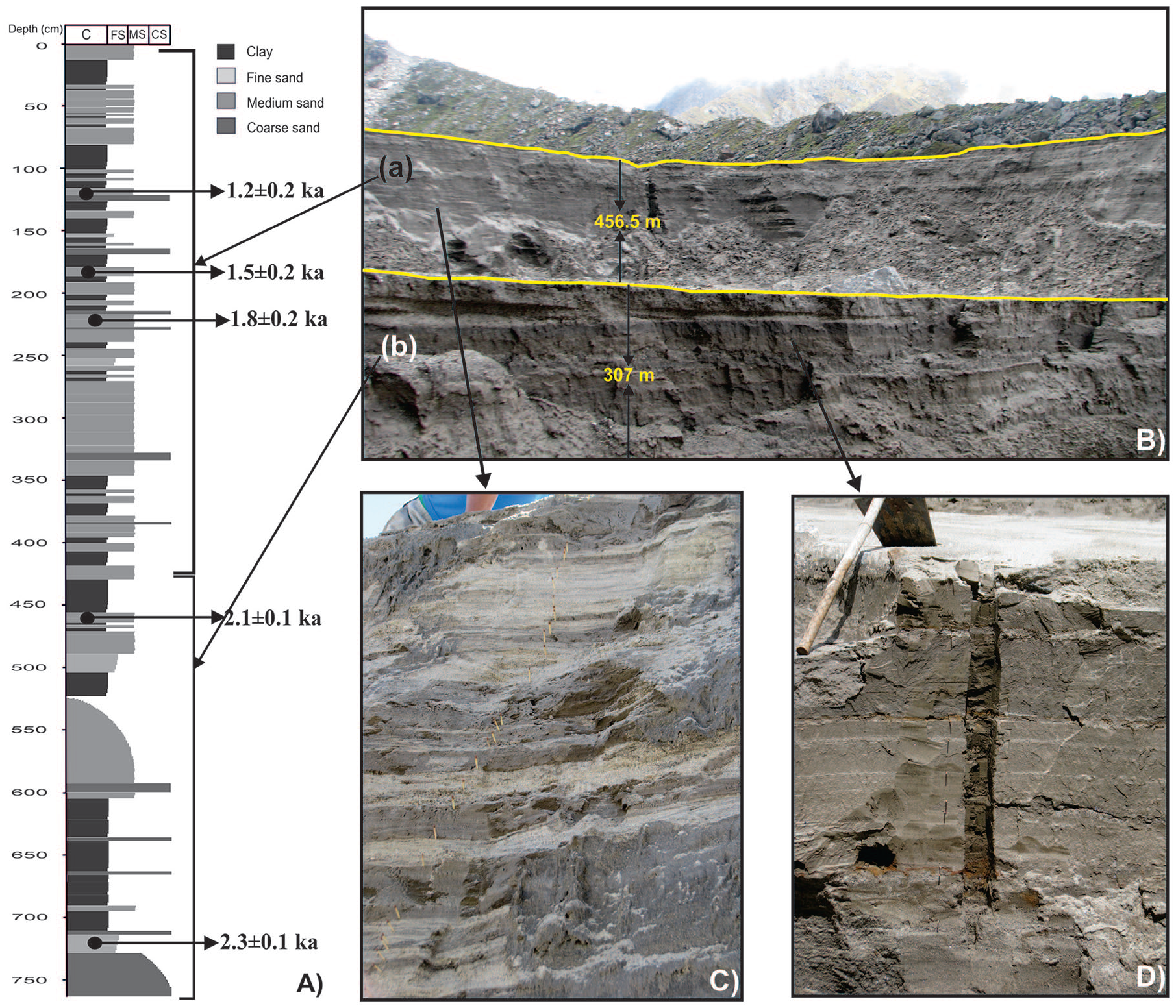
(A) Lithology of the exposed section of the lake sequence. (B) Field photographs showing the 8-m complete section of lake sequences. (C, D) Close-up view of lake sequence, showing the alternative band of sand and clay.

On the basis of lithostratigraphy, we categorized the exposed lake sediment into four distinct units from bottom to top. The bottom Unit I of the lake sequence between 601 and 763 cm is characterized by gravel, clay and coarse sand interbedded with patches of medium and fine sand. The lowermost part of the lacustrine sequence comprises 35-cm-thick matrix-supported angular gravels followed by 14.5 cm layer of fine sand and 106 cm of clay with two intervening sand layers of 3 and 4 cm, respectively (Figure 4A).

This is succeeded by a 200-cm-thick sequence of Unit II between 401 and 600 cm composed of medium-grained sand, clay and silt. The bottom of this section comprises 7 cm coarse sand followed by 69 cm medium sand layer and 19 cm clay bed. The sequence is followed by 47 cm fine and medium sand layer interbedded with 2–3 cm clay bed (Figure 4A). The top of this unit comprises 27-cm-thick clay deposit.

The 200-cm-thick Unit III sequence between 201 and 400 cm is predominantly composed of medium to coarse graded sand interbedded with thin (4–5 cm) bands of laminated clay (Figure 4A). This type of deposition suggests fast settling of fine-grained particles under medium- to high-density turbid flow conditions. Also, episodes of enhanced sediment shedding like this denote high-energy conditions in the lake during the time of deposition.

The uppermost 200-cm-thick sediment Unit IV mainly consists of fine-grained, brown and dark grey silty clay and clay, with intervening sand layers (Figure 4A). This lithostratigraphic unit, which is fine-grained, indistinctly laminated, bioturbated, shows lack of sorting, and the absence of sedimentary structures indicates that the sedimentary deposition in the lake occurred in low-energy environment. Dispersed sand grains depict that the sediment transport took place in high-energy stream flow conditions. The contact between Units III and IV occurs over a 10-cm-thick transitional zone composed of thin layers of massive, matrix-supported sand (Figure 4).

Sampling strategy and chronology – optically stimulated luminescence (OSL) dating

A total of 101 sediment samples (random interval) were collected for mineral magnetism, mineralogical and chemical changes (XRF), and grain size studies. We also collected five samples from the sediment column (base to top of column) for OSL dating. The samples were taken from 15-cm-thick opaque pipes with 2.5 cm diameter drilled into the exposed lake sediment section at five different height intervals. Also, by the same technique, two samples were collected from the base of the moraine to determine the timing of the Chorabari Lake formation. The lake succession was formed by an alternative band of sand and clay, which represent dry and wet weather conditions in the lake environment (Figure 4C and D). Samples of sand and clay were collected in airtight plastic bags.

For calculating the OSL ages, we have extracted pure quartz after sequential pretreatment involving removal of carbonate and organic carbon by 10% HCl and 30% H₂O₂, sieving and density separation using sodium polytungstate (2.58 g/cm³). Furthermore, the alpha-effected skin of quartz grains was etched using 80 min of HF followed by 30 min of 12 N and HCl treatment. Infrared stimulated luminescence (IRSL) measurement was performed on every sample to check feldspar contamination. The samples showing IRSL counts more than 100 counts/0.40 s were subjected to the additional step of density separation and HF etching for 20 min. Finally, stainless steel discs (9.65 mm diameter) were used to mount clean quartz grains using Silko-Spray silicone oil. The equivalent dose was determined using SAR protocol based on Murray and Wintle (2000). All the analyses were performed using an Risø TL/OSL DA-12 automated luminescence reader system equipped with a Sr-90 beta irradiator (6.7 Gy/min). The OSL emission was stimulated by blue LEDs with 90% optical power and was detected by EMI 9235 QA photomultiplier for photon detection with attached Schott BG-39 and Hoya U-340 optical filters.

The preheat temperature was set to 220°C/10 s and the cut-heat temperature to 160°C. Thirty to thirty-five discs were used for palaeo-dose measurement, of which the weighted mean of the lowest 20% palaeo-dose values was used for age calculation (Mehta et al., 2012; Ray and Srivastava, 2010). The typical regeneration growth curves are shown in Figure 5. The x-ray fluorescence analysis was used to determine the concentration of Uranium (²³⁸U), Thorium (²³²Th) and Potassium (K; Wintle, 2008). The OSL measurements were performed for 40 s at 125°C, and the data were analysed using the Analyst software (Duller, 2008).

Figure 5.

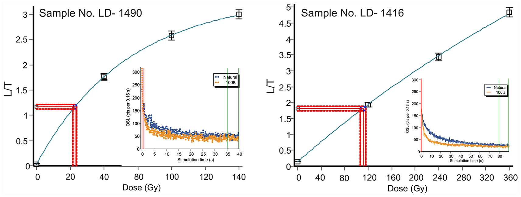
Plotted graph shows typical growth curve for the sample numbers LD-1490 and LD-1416. The inset figure represents the shine-down curve of respective samples.

Glacier samples suffer from low sensitivity, feldspar contamination and partial bleaching problems, and these samples are no exception. The samples analysed show low sensitivity and a bleaching problem. The feldspar contamination was not an issue as it was resolved by checking IRSL on each aliquot, and if it was very low (e.g. almost at background level), then it was selected for applying SAR. The samples in a glacier environment have a high chance of partial bleaching due to very short transport distances and also thick ice moves carrying sediments, which may attenuate daylight to a great extent. We applied different age models and found that least 20% fits with the stratigraphy and has been widely used in OSL dating for sediments deposited in the similar mountainous environment (Ray and Srivastava, 2010; Srivastava et al., 2009). The distribution of equivalent dose (De) values is presented in radial plots and probability distribution plots (Figure 6).

Figure 6.

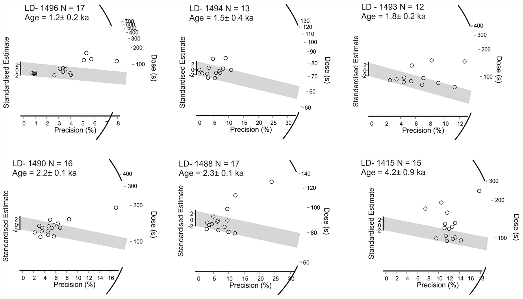
The distribution of equivalent doses (De) values for all samples presented with radial plots and probability distribution curves. Shaded part of the radial plot highlights the discs used for measurement and the inset in probability distribution plot shows the minimum number of samples discs which were exposed to sunlight before burial. Discs falling in the shaded part were used for age calculation

Furthermore, the Uranium–Thorium disequilibrium is also an important issue to discuss as leaching of sediment under water-saturated conditions might be considered for lake sediment dating. The movement of water through sediment can affect the concentrations of more soluble isotopes and lead to disequilibrium of the isotopes in the Uranium and Thorium decay chains. Water is also responsible for the dissolution and re-precipitation of carbonate in sediments, and this will also affect the dose rate through time. However, the sediments we dated show (1) no obvious signatures of leaching or water percolation (except LD-1490), and (2) the isotopic ratio of U–Th is near 3–7 (which is natural), with K contributing 60–70% of the dose; hence, the effects of disequilibrium allow us to assume radioactive equilibrium for most of the samples.

Particle size analysis

The grain size of the samples less than 1 mm in diameter was analysed by the laser particle size analyser, that is, Mastersizer 2000MU (particle size: 0.02–2000 µm, accuracy: better than 1% (polydisperse standard), reproducibility: better than 1% variation (polydisperse standard)) along with the wet dispersion unit Hydro-2000. The instrument calculates the volume percentage of sample and divides it into different class intervals according to the distribution of different sizes of grains. Samples that are more than 1 mm in diameter were studied using sieving and pipette analysis.

Environmental magnetic parameters

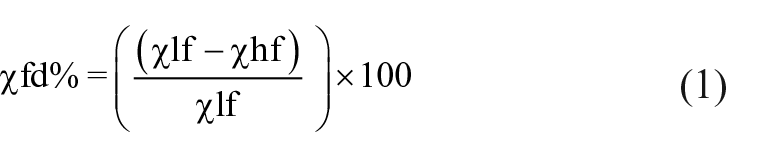
To determine the concentration of grain size and magnetic minerals, the samples were first packed into 10 cm³ non-magnetic styrene pots. The magnetic susceptibility (χlf) was measured with duel frequency sensors (0.47 and 4.7 kHz) using a Bartington MS-2B magnetic susceptibility meter. The percentage frequency dependence susceptibility χfd% is calculated using the following formula:

χ fd % = (\frac{(χ lf - χ hf)}{χ lf}) \times 100

(1)

Isothermal remnant magnetization (IRM) was measured by a forward magnetic field of 20, 50 and 100 to 2200 mT in an impulse magnetizer at 100 mT incremental sequences. A backward magnetic field of 10, 20, 30, 50, 100, 300 and 400 mT was also imposed to demagnetize the sample. The magnetic moment was measured by the Minispin rock magnetometer of Molspin, UK. The IRM1200 is referred to as saturation isothermal remnant magnetization (SIRM). Anhysteretic remnant magnetization (ARM) was grown with a peak alternating field of 100 mT in the presence of a DC field of 0.1 mT. S-ratio was calculated from the remnant magnetization in a negative field of 300 T and divided by SIRM (IRM_{−300 T}/SIRM) (Stober and Thompson, 1979).

Environmental magnetism has been extensively used to examine the sedimentation pattern based on the relationship between mineral magnetic properties and changes in climatic conditions controlling them. This magnetic mineralogy coupled with particle size distribution becomes sensitive particularly for changes in sediment profiles (Oldfield et al., 1985). Considering the phenomenon of glacial retreat and advancement in the valley, two potential candidates for cause of variations have been recognized: first, the periods of glacier retreat, marked by higher glacial sediment output, and second, the ice-covered conditions to the lake which infers low inputs from basal flow.

The sediments (and magnetic minerals) derived from the catchment are modified through the climatic fluctuations and the sediment characteristics should, in principle, reflect the changing balance between glacially derived sediments and sediments originating from wide variety of substrates, including bedrock, glaciofluvial deposits and moraines. The process of mineral magnetic deposition in lake profile was influenced by four major variables: (1) the concentration of ferri/ferromagnetic iron oxides in the catchment; (2) the relative contribution of different ferri/ferromagnetic phases (e.g. magnetite and hematite); (3) the size of the particles and (4) the relative contribution of paramagnetic minerals (e.g. biotite and pyrite) and diamagnetic minerals (e.g. quartz and water). A possible interpretation of the data follows as in periods of climatic transition, the supply of minerogenic material to lakes is reduced and the sediment with a lower organic content were deposited. A slow deposition rate could also lead to magnetite dissolution, resulting in a low magnetic concentration and high S-ratio. Conversely, during periods of glacial retreat, the minerogenic sedimentation rate increases and magnetite is preserved in the sediments because of rapid burial, which results in a high magnetic concentration and low S-ratio.

Elemental analysis

For major oxides, 5 g of sample was ground to a fine powder, mixed with two to three drops of polyvinyl alcohol solution. A hydrologic pressure of 2000 kg cm⁻² was used for palletizing the sample powder to make a ~3.5-mm diameter pellet backed with boric acid layer. Subsequently, the pellets were kept in a hot box (60–70°C) overnight to drive off the excess water from the binder. Finally, the pellets were kept inside the x-ray fluorescence spectrophotometer for determining the weight % oxides (SiO₂, TiO₂, Al₂O₃, Fe₂O₃, MnO, MgO, CaO, Na₂O, K₂O and P₂O₅) in geological matrices and trace elements (Ba, Sc, V, Cr, Co, Ni, Cu, Zn, Ga, Pb, Th, Rb, U, Sr, Y, Zr and Nb) at >5 ppm (2 ppm for some elements) level. Accuracy was tested as per international standards which are detailed in Purohit et al. (2010) and Saini et al. (2002).

The geochemical properties of lake sediments have been tested with the plots of element percentage versus depth in the sediment column. It has been interpreted that the high percentage of Na ⁺, Ca^{2 +} and Mg^{2 +} cations indicates humid climate (Engstrom and Wright, 1984; Newman, 1987), and also the oxides of SiO₂ and Al₂O₃ and their relative percentages signify wetter/warmer (humid) climatic conditions (Newman, 1987). The Fe/Mn ratio is generally regarded as a proxy for redox conditions at the lake bottom (Rush, 2010). High Fe/Mn ratio infers higher solubility of Mn under reducing conditions (Boyle, 2001). Ca/Mg ratio represents the arid–wet climatic condition as Ca leaches more readily in humid climate because of large ionic radii (Huang et al., 1982). Na/Al ratio is used as indicator of weathering degree (Ding and Ding, 2003). Since the Chemical Index of Weathering (CIW) and Chemical Index of Alteration (CIA) give the same trend (R² = 0.97), we have plotted only CIA in the present work.

Sources of errors

We have applied a multiproxy approach to the glacier-fed Chorabari Lake and inferred the catchment processes governed by ameliorating climatic conditions. Considering the sensitivity of glacial environment towards climatic perturbations, we have interpreted our results as the sediments deposited in the lake have preserved similar physical/chemical imprint pertinent to climatically induced catchment processes. We caution against generalized interpretations of mere coincidence of out-of-phase relation of climatic perturbations and focussed on casual correlations to interpret our results.

Results and discussion

Chronology of climatic events

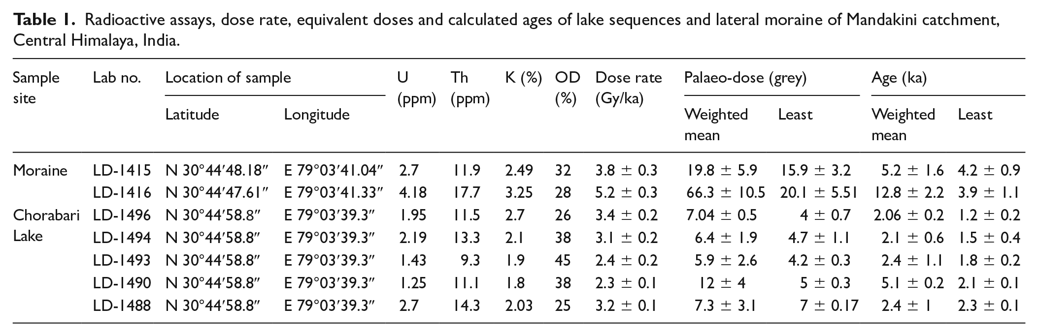
The lateral moraine of Chorabari Glacier blocked the stream flow and created the Chorabari Lake (Figure 2). The OSL chronology from the base of lateral moraine suggests that the moraine was formed between 4.2 ± 0.9 and 3.9 ± 1.1 ka. The widespread 4.2 ka cooling (DeMenocal, 2001; Staubwasser et al., 2003) may be correlated with the last stage of glacial advancement in the Mandakini River Basin, Central Himalaya, between ~5 and 4 ka, suggesting that the Chorabari Lake was formed between ~5 and 2.3 ka. There is no complete or fragmented moraine ridge present above this moraine ridge to suggest further major event of glaciations in the valley.

In addition, the lake stratigraphy is dated with OSL chronology of five samples collected from the exposed lake section (Figure 4, Table 1). The sediment layer close to the bottom of the section at 763 cm is dated to ~2.3 ± 0.1 ka, followed by the top layer about 168 cm from the surface dated at ~1.2 ± 0.2 ka. The age–depth model (Figure 7) and sediment records indicate that three major events occurred between 2.3 ka and the present day. Since the lake strata has preserved rapid sedimentation, which might be possible through steep slope of the valley, the multiproxy data presented here indicate many rapid climatic fluctuations. Therefore, we have divided the stratigraphy into three major phases based on climate imprint of the proxy data, that is, (1) 260 BCE and 270 CE, (2) 900 and 1260 E and (3) ~1370 and 1720 CE. Considering the age–depth model and variability of environmental magnetic properties, the lake chemistry of ~8 m profile has been subdivided into three sections as follows.

Table 1.

Radioactive assays, dose rate, equivalent doses and calculated ages of lake sequences and lateral moraine of Mandakini catchment, Central Himalaya, India.

Sample site	Lab no.	Location of sample		U (ppm)	Th (ppm)	K (%)	OD (%)	Dose rate (Gy/ka)	Palaeo-dose (grey)		Age (ka)
Sample site	Lab no.	Latitude	Longitude	U (ppm)	Th (ppm)	K (%)	OD (%)	Dose rate (Gy/ka)	Weighted mean	Least	Weighted mean	Least
Moraine	LD-1415	N 30°44′48.18″	E 79°03′41.04″	2.7	11.9	2.49	32	3.8 ± 0.3	19.8 ± 5.9	15.9 ± 3.2	5.2 ± 1.6	4.2 ± 0.9
Moraine	LD-1416	N 30°44′47.61″	E 79°03′41.33″	4.18	17.7	3.25	28	5.2 ± 0.3	66.3 ± 10.5	20.1 ± 5.51	12.8 ± 2.2	3.9 ± 1.1
Chorabari Lake	LD-1496	N 30°44′58.8″	E 79°03′39.3″	1.95	11.5	2.7	26	3.4 ± 0.2	7.04 ± 0.5	4 ± 0.7	2.06 ± 0.2	1.2 ± 0.2
	LD-1494	N 30°44′58.8″	E 79°03′39.3″	2.19	13.3	2.1	38	3.1 ± 0.2	6.4 ± 1.9	4.7 ± 1.1	2.1 ± 0.6	1.5 ± 0.4
	LD-1493	N 30°44′58.8″	E 79°03′39.3″	1.43	9.3	1.9	45	2.4 ± 0.2	5.9 ± 2.6	4.2 ± 0.3	2.4 ± 1.1	1.8 ± 0.2
	LD-1490	N 30°44′58.8″	E 79°03′39.3″	1.25	11.1	1.8	38	2.3 ± 0.1	12 ± 4	5 ± 0.3	5.1 ± 0.2	2.1 ± 0.1
	LD-1488	N 30°44′58.8″	E 79°03′39.3″	2.7	14.3	2.03	25	3.2 ± 0.1	7.3 ± 3.1	7 ± 0.17	2.4 ± 1	2.3 ± 0.1

Figure 7.

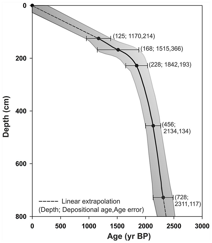
Age–depth model for the Chorabari Lake profile. Shaded part envelops the relative age error in optically stimulated luminescence dating, and dashed line represents the liner extrapolation of ages.

Section I (270 BCE–~260 CE)

This section presents the sedimentation with low χlf values from ~260 CE to ~270 BCE, with the presence of antiferrimagnetic minerals, except two peaks at ~170 BCE and~40 CE showing the presence of ferrimagnetic minerals (Figure 8). χARM also follows the same trend, showing the presence of multi-domain (MD) grains along with antiferrimagnetic minerals and SP grains with ferromagnetic minerals. Whereas the S-ratio shows an opposite trend, with positive values (maximum 0.19 to minimum −1.0) confirming the presence of hematite mineral. The χfd% shows higher values (+5.88 m³ kg⁻¹) at~164 BC followed by a gradual decrease till ~200 CE (Figure 8). This section indicates some interesting results as a sudden decrease in χlf and χARM values between –150 BC and 40 CE has opposite and positive trend in S-ratio, indicating high input of detrital sediments under reducing environmental conditions. A gradual increase at ~40 CE shows an increase in the magnetic enhancement during cold and dry periods, and then a sudden decrease is observed in the data which continues from ~50 to 250 CE, suggesting that χlf also decreased due to the absence of magnetic enhancement, increasing detrital titanomagnetite concentration, produced in situ by low-temperature oxidation during a wet and cold climate condition. The increased grain size in this section also supports the high detrital input to lake through increase in subglacial meltwater stream.

Figure 8.

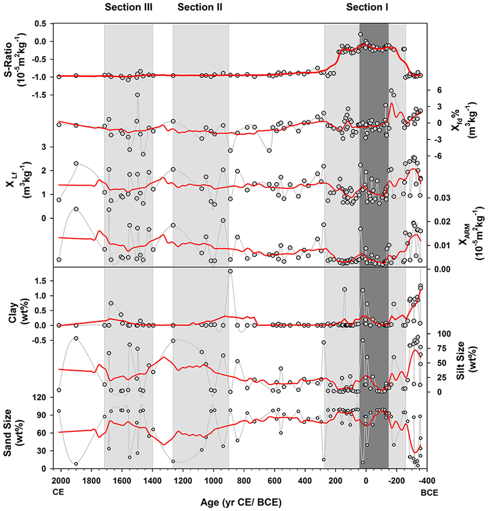
Environmental magnetism and grain size proxies plotted against lake chronology. The shaded part indicates different sediment deposition patterns with respective climatic conditions at the lake for a specific time period. The mean climate state of representative proxy response is marked in red and calculated with 2D smoothening of the data using sigma plot software version 14.

Geochemistry of this section corresponds to moderate to low CIA, LOI, Fe₂O₃ with high to low Fe/Mn, Ca/Mg, Na/Al, Na₂O%, SiO₂%, K₂O% and Al₂O₃% values showing the transition of arid/warmer climate to cold and dry conditions at ~0–200 CE. Low Al₂O₃, Fe₂O₃, Ti, Fe/Mn ratios and high Na₂O, Ca/Mg, Na/Al ratios suggest poor chemical weathering under deprived precipitation and deteriorating climatic conditions (Figure 9).

Figure 9.

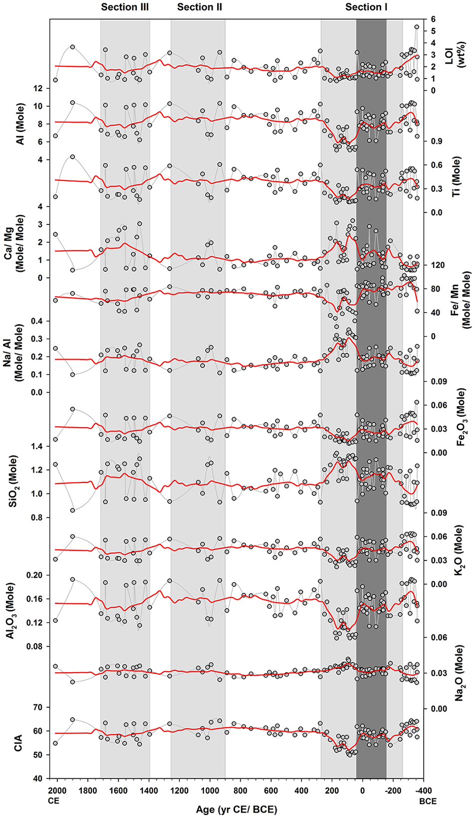
Geochemical proxies plotted against lake chronology. The shaded part indicates different sediment deposition patterns with respective climatic conditions at the lake in specific time interval. The mean climate state of representative proxy response is marked in red and calculated with 2D smoothening of the data using sigma plot software version 14.

The section corresponds to a few earlier suggestions of arid and cold events between 2.2 ka BP (–187 BCE) and 1.8 ka BP (213 CE) (Chauhan et al., 2010; Yadava and Ramesh, 2005). A cool and dry climate state during 2 ka has been observed due to large-scale weakening of the southwest monsoon system. Furthermore, the speleothem record from Pokhra valley, Nepal, suggested that between 2.3 ka (–287 BCE) and 1.5 ka (513 CE), the summer monsoon precipitation was diminished (Denniston and González, 2000). Similar cold and dry climatic conditions were documented in the Pindari valley, Kumaon, Higher Himalaya, between 2.1 ka (–87 BCE) and 1.6 ka (413 CE), probably representing the coldest and driest events of the past 3500 years (Bali et al., 2013; Phadtare, 2000). The multiproxy data from lake sediment record for Chorabari Lake also suggest an overall cooler phase of sedimentation in the valley. Therefore, after lake formation, the lake has experienced the cooler conditions till 1.8 ka (213 CE) coupled with reduced precipitation conditions.

Section II (~900-1260 CE)

The magnetic data of this section indicate a wet and cold phase during ~1000 CE when concentration of MD grains along with sand-mixed clay deposits increased. Since then, climate gradually became warm and humid until ~1200 CE. In this section, the magnetic susceptibility values range from a maximum of 2.04 × 10⁻⁸m³ kg⁻¹ at ~1260 CE and a minimum of 0.57 × 10⁻⁸m³ kg⁻¹ at ~990 CE. The susceptibility values initially increased to 2.03 × 10⁻⁸m³ kg⁻¹ at ~935 CE, showing the presence of ferromagnetic minerals which suddenly decreased to minimum level at ~1015 CE (Figure 8). This sudden increase in susceptibility is coupled with an increase in silt-sized particles, indicating a sudden shift from drier to wetter conditions. Also, the sudden decrease in susceptibility values at ~990 CE could have resulted due to an increased organic matter mixed with sediment and water. Furthermore, the χARM values followed the same trend showing the presence of SSD grains at ~935 CE and then suddenly decreased to MD minerals at ~1015 CE. However, a significant change in S-ratio of samples has been observed with average negative values of 0.95 × 10⁻⁵m² kg⁻¹ showing the presence of magnetite mineral grain. The occurrence of very small magnetic grains of stable single domain (SSD) boundary gives rise to χfd%; however, the χfd% values are low throughout the section. A smaller fluctuation in χfd% values until ~1077 CE and then a gradual increase are observed towards positive values (Figure 8). The magnetic data of this section indicate a wet and cold phase during ~1000 CE, and during this time, the concentration of MD grains along with sand-mixed clay deposits increased and since then it gradually changed towards warm and humid phase of climate until ~1200 CE. There are no significant variations observed in the data, and overall it indicates a warm and humid climate with an anomaly at ~1000 CE.

The geochemistry of this section supports the magnetic data, having moderate to high CIA values, decreasing trend from high to low Na₂O, Na/ Al, Ca/Mg, and SiO₂, and increasing trends from low to high K₂O, Al₂O₃, and Fe/Mn ratios. It suggests high chemical weathering in the catchment and warm/humid conditions at the Chorabari Lake. However, an opposite trend has been observed at ~1050 CE, indicating increased erosion under high precipitation conditions (Figure 9).

Based on our results, this phase of sedimentation could be correlated with global MCA event (Crowley and Lowery, 2000; Ledru et al., 2013; Mann et al., 2009). Comparing our results with the Triloknath Lake sediment record, the climatic conditions show similar episodes of warmer phase depicted from enhanced antiferromagnetic mineralogy and higher CIA values recorded between 1200 and 1350 CE (Bali et al., 2017). Similarly, the other studies in the Himalaya indicate warm and wet (humid) MWP in the region between 800 and 1350 CE (Chauhan et al., 2000; Mazari et al., 1996; Phadtare and Pant, 2006). The time of warm climate in the North Atlantic and its footprints have been observed around the world lasting generally from ~950 to ~1250 CE. Moreover, Dasuopu ice core records suggest that the warm period lasted from 1140 to 1360 CE, which corresponds to the MCA on the southern part of the Tibetan Plateau (Yang et al., 2002, 2007a,2007b).

Section III (~1370–1720 CE)

In this section, magnetic susceptibility has a minimum value of 0.615 × 10⁻⁸ m³ kg⁻¹ at ~1460 CE and a maximum value of 2.04 × 10⁻⁸m³ kg⁻¹ at ~1685 CE, which is followed by the lowermost value from 0.9 to 0.7 × 10⁻⁸m³ kg⁻¹ during ~1595–1670 CE. This gradual increase and decrease in values indicate the presence of both ferromagnetic and antiferromagnetic minerals between ~1370 and 1720 CE corresponding to the ‘Little Ice Age’ (LIA) (Figure 8). The same trend is followed by χARM values falling in this zone and shows the presence of SSD and super-paramagnetic (SP) and MD grains which are dependent directly on size and complex spin patterns of electrons and indirectly on time and temperature. We observed minor fluctuation in S-ratio of mineral grains showing negative values from maximum to minimum (–1.08 to 0.84 × 10⁻⁵m² kg⁻¹) and indicating magnetite mineral deposition in oxidizing environment. Similarly, χfd% in this section shows more negative values ranging from ~–2 to −6 m³ kg⁻¹ except a positive value of + 5.12 m³ kg⁻¹ depicts warm and humid phase of climate (Figure 8). The magnetic data indicate that the concentration of mineral was initially low during ~1470 CE and then gradually increased at ~1500 CE. The sudden decrease in the MD and single domain (SD) grains is also supported by sediment grain size data. This sediment section represents the absence of magnetic enhancement during the wet climate and low-temperature oxidation.

The lake chemistry in this section is characterized by low CIA, Al%, Ti%, Fe/Mn, K₂O, Al₂O₃, LOI, Fe₂O₃ values and high Na₂O, Na/Al, Ca/Mg values, indicating low weathering under cold climatic conditions with low organic productivity. However, at ~1500 and 1550 CE, a sudden rise in these values denotes stronger hydrodynamics and moderate weathering conditions (Figure 9).

This section is characterized by conditions similar to the LIA as this interval was a distinct event intermittent with small phases of warm and cold episodes, as evidenced in other parts of the Himalaya and the world (So Bali et al., 2017; Bhattacharyya et al., 2007; Mann et al., 2009; Soon and Baliunas, 2003). The LIA is a short-lived period of widespread cooling in the northern hemisphere characterized by mean annual temperature change of about –0.5°C with lowest temperature between 1400 and 1700 CE (Mann et al., 2009; Wilson et al., 2016). The LIA represents the last glacial advancement at the Himalaya. However, the Gangotri Glacier in the Central Himalaya shows an advancement during 1700–1800 CE (Barnard et al., 2004a), whereas the Jaundhar and Bandarpunch glaciers advanced during 1400 and 1700 CE (Scherler et al., 2010). The ice core of East Rongbuk Glacier suggested that the mean glacier accumulation rate was 0.8 m w.e.a⁻¹ between 1500 and 1600 CE (Kaspari et al., 2008). The ice core record suggests an abrupt southward shifting event of the South Asian monsoon around 1400 CE. These high-altitude ice cores and other proxies collected from the Himalayan region indicate increased precipitation at ~1400 CE as the monsoon moved southward, accompanied by cooler temperature and increase in westerly winter precipitation (Kotlia et al., 2012, 2015; Liang et al., 2015; Phadtare and Pant, 2006). The glacier advance in the Central Himalaya during the LIA coincides with the hemispheric temperature records, suggesting that these stages result from variations in the westerlies (Murari et al., 2014). This last period of the Holocene (LIA) occurred with the greatest cooling over the extratropical Northern Hemisphere (Mann et al., 2009). Furthermore, the post-LIA climate change, glacier ice loss and glacier retreat have also been documented in all parts of the high-altitude (mountainous) and high-latitude (arctic) regions (Barry, 2006; Overpeck et al., 1997).

Regional correlation of glacial fluctuations

Owing to the large geographical extent with complex and extreme topography, influenced by ISM and MLW circulation, the Himalayan glaciers present a unique opportunity to study and understand the climatic changes preserved in the form of glaciations. Recent studies explaining the glaciation patterns of Himalaya have suggested a complex interplay of precipitation and temperature for Himalayan region (Ali et al., 2013; Owen and Dortch, 2014; Shukla et al., 2017, 2018; Zech et al., 2009). The topographic influence to the climate system has hardened any single explanation about the timing and extent of glacial advances (Lehmkuhl and Owen, 2005; Rowan, 2017). Therefore, we compiled the regional chorology from Central Himalayan region encompassing glacierized valleys of Indian and Nepal Himalayas and compared with the climatic history of the Chorabari Glacier. The Be10 and OSL chronology of the different valley systems suggests that the glaciation between 2 ka (13 CE) and 1.5 ka (513 CE) was largely scattered (Figure 10). Only 04 OSL and 05 Be10 dating-based glaciation records were present, although it is interesting to note that these records are majorly from the regions that are precipitation deprived – for example, the Kosa valley (Bisht et al., 2017), Upper Dhauliganga valley (Bisht et al., 2015) and Nanda Devi region (Barnard et al., 2004b) situated in precipitation-dominated regions and much sensitive to glaciation in response to change in precipitation than temperature (Batbaatar et al., 2018). Section I of our lake records suggests a cooler and monsoon weakening conditions till 1.8 ka (213 CE); thereafter, monsoon strengthening was observed, so possibly the glaciation during this time was only limited to the regions sensitive to precipitation. Furthermore, the altitudinal effect of glaciation as suggested by Figure 10(B) could be considered here, as the asynchronicity in Himalayan glaciations driven by orographic sensitivity has already been proven (Pratt-Sitaula et al., 2011). Section II presented in our lake climate record does not appeal much in terms of glaciation events of Central Himalayan region, as barring the precipitation-dominated regions explained above has only preserved the glaciation events. The frequency distribution of OSL ages suggests the glaciation in Kosa and upper Dhauliganga valleys. The hypothesis presented above can be successfully applied to this period as the lake climate suggests warm and humid conditions, leading to monsoon enhancement in the Central Himalayan region and producing favourable environment for glaciation in precipitation-deprived regions.

Figure 10.

The distribution of moraine ages assigned to glacier advances during the last 3 ka in the Himalaya shown as (A) probability density plot of glaciation chronologies; blue bars represent Be 10 chronology, while red bars represent OSL chronologies, (B) altitudinal distribution of ages and (C) comparison of glaciation chronologies from different parts of the Himalaya. The green circles represent Be 10 chronology, while the red circles represent OSl chronology. The errors in chronology are presented with grey colour. (a) Bhilangna and Dudhganga valley (Murari et al., 2014), (b) Mayali and Kedarnath valleys (Murari et al., 2014), (c) Tons valley (Scherler et al., 2010), (d) Nanda Devi valley (Barnard et al., 2004b), (e) Dudh Kola and Marsyangdi valley (Zech et al., 2009), (f) Dokriani valley (Shukla et al., 2018), (g) Khumbu Himalaya (Richards et al., 2000), (h) Kosa valley (Bisht et al., 2017), (i) Upper Dhauliganga valley (Bisht et al., 2015) and (j) Dhauliganga valley (Kumar et al., in review).

The last phase of glaciation during LIA presented in section III has preserved ample glaciation evidence in the Central Himalayan region. The frequency plot and age distributions during this time are preserved in all precipitation-dominated valleys. The lake climate reconstruction suggests the cooler conditions with occasional high precipitations. Since the glaciations in the monsoon-dominated regions having precipitation dominance are much sensitive to changes in temperature than precipitation (Shukla et al., 2018, 2019; Zech et al., 2009), we can correlate that the large glaciation event occurred in the Central Himalayan region with the cooler environment and variable conditions during LIA. An extensive review presented by Rowan et al. (2017) has suggested that the LIA glacial advancement of Himalaya was largely correlated with the Northern Hemisphere temperature changes led by low insolation, which is also reflected in climatic reconstruction of the Chorabari glacial lake and climatic conditions for the region. Here, it could be suggested that the glacier expansion in the region was dictated by low insolation with corresponding radiative forcing, leading to cooler temperature.

In addition, the Chorabari glacial valley has been previously investigated for the major glaciation advancement of the valley (Mehta et al., 2012). Briefly, four major glacial stages have been identified, characterized as Rambara glacial stage (RGS; 13 ± 2 ka), Ghindurpani glacial stage (GhGS; 9 ± 1 ka), Garuriya glacial stage (GGS; 7 ± 1 ka) and Kedarnath glacial stage (KGS; 5 ± 1 ka). RGS was the most extensive glaciation extending for ~6 km down the valley from the present day snout of the Chorabari Glacier and down to an altitude of 2800 m a.s.l. at Rambara covering around ~31 km² area in the Mandakini Valley. The OSL chronology of the lateral moraine bounding the Chorabari Lake suggests its formation between 4.2 ± 0.9 and 3.9 ± 1.1 ka corresponds to the last major glaciation in the Mandakini Valley which occurred between 5 and 4 ka (Table 1). This youngest chronology of the valley (~4 and 5 ka) is coeval with ~4 ka cooling event of the Dunde ice core records from the Tibetan Plateau (Thompson et al., 1989). The effect of climate cooling during 4–3 ka caused glacier advancements in different regions. Zheng et al. (2002) and Finkel et al. (2003) recognized a glacial advance in the Xuedong, southern Tibet, at ¹⁴C age of 3 ± 1.5 ka and in Khumbu glacier (Tukhla glacier stage) in the Nepal Himalaya at ~3.6 ka, respectively. Farther west, glacial advance has been recorded in the Bagni Glacier (7.5–4.5 ka) and Pindari Glacier (6–3 ka) in the Alaknanda basin of the Central Himalaya (Bali et al., 2013; Sati et al., 2014). The glacial advancement in the valley was well correlated with the regional glaciation events of Central Himalaya. Our lake sediment records at Chorabari Glacier could be identified as an excellent proxy to explain the detailed explanations for the glaciation events occurring in the monsoon-dominated regions of the Himalaya.

Conclusion

Environmental magnetic, sedimentological and geochemical records coupled with OSL chronology of moraine and lake sediments were used to reconstruct climatic variability and subsequent glacial sensitivity in the Mandakini River Basin, Garhwal Central Himalaya, during the late Holocene. The lake morphology suggests that the Chorabari Lake is moraine-dammed and experienced numerous glacial and deglacial phases in the valley. The OSL chronology suggests that a set of moraine deposition occurred between 4.2 and 3.9 ka, leading to the accumulation of ~8 m of lake strata during the past 2.3 ka. Based on the proxy records from the Chorabari Lake stratigraphy, we suggest that the Mandakini Valley experienced three major events between 2.3 ka and the present. On the basis of the proxy records and age–depth model, the following events could be summarized:

270 BCE to 260 CE. This event represents fluctuation in the climatic conditions between cool and dry to hot and humid climate, and ~0 BC is probably the starting of neoglaciation period in the Himalaya.

900 to 1260 CE. Our records show that this event in the Mandakini Valley coincides with the medieval climate anomaly as witnessed all over the world.

1370 to 1720 CE. This event corresponds to the LIA, showing a distinct event with intermittent warming and cooling episodes as evidenced in other parts of the Himalaya and the world.

The OSL dates suggest that the last stages of glacial advancement in the Mandakini basin occurred during ~5–4 ka, which infers that the Chorabari Lake was formed between ~5 and 2.3 ka.

Considering the global glacial retreat in global warming scenario, the high-resolution climate records in the vicinity of glaciers are important. The glacial feedbacks to the climate system are significant to consider as interpreting the glacier–climate interactions in more effective ways. This becomes particularly important if regional or local phenomena are explained. We believe that the rapidly growing studies like the present one explaining the glacial–climate feedback mechanism will answer the drivers of these natural climate systems.

Footnotes

Acknowledgements

The authors gratefully acknowledge Department of Science and Technology (DST), New Delhi, and Wadia Institute of Himalayan Geology (WIHG), Dehradun, for providing financial support and facilities to carry out this work. MM wishes to express his gratitude to professor A K Gupta for his valuable guidance. The authors sincerely thank Dr. Akshya Verma, Dhanveer and Pratap Singh, Centre for Glaciology, WIHG, for their help during the sample collection. They also like to sincerely thank the anonymous referees for their constructive comments and insightful suggestions, which considerably improved the manuscript.

Funding

The author(s) received financial support from Department of Science and Technology (DST), New Delhi, and Wadia Institute of Himalayan Geology (WIHG), Dehradun for the research, authorship and/or publication of this article.

ORCID iD

Tanuj Shukla

References

Ali

Biswas

Shukla

, et al. (2013) Chronology and climatic implications of Late Quaternary glaciations in the Goriganga valley, central Himalaya, India. Quaternary Science Reviews 73: 59–76.

Armstrong

(2010) The Glaciers of the Hindu Kush-Himalayan Region – A Summary of the Science Regarding Glacier Melt/Retreat in the Himalayan, Hindu Kush, Karakoram, Pamir, and Tien Shan Mountain Ranges. Kathmandu: ICIMOD, p. 17.

Bali

Ali

Agarwal

, et al. (2013) Chronology of late Quaternary glaciation in the Pindar valley, Alaknanda basin, Central Himalaya (India). Journal of Asian Earth Sciences 66: 224–234.

Bali

Khan

Sangode

, et al. (2017) Mid- to late-Holocene climate response from the Triloknath palaeolake, Lahaul Himalaya based on multiproxy data. Geomorphology 284: 206–219.

Barnard

Owen

Finkel

(2004a) Style and timing of glacial and paraglacial sedimentation in a monsoon-influenced high Himalayan environment, the upper Bhagirathi Valley, Garhwal Himalaya. Sedimentary Geology 165: 199–221.

Barnard

Owen

Sharma

, et al. (2004b) Late quaternary (Holocene) landscape evolution of a monsoon-influenced high Himalayan valley, Gori Ganga, Nanda Devi, NE Garhwal. Geomorphology 61(1–2): 91–110.

Barry

(2006) The status of research on glaciers and global glacier recession: A review. Progress in Physical Geography 30(3): 285–306.

Batbaatar

Gillespie

Fink

, et al. (2018) Asynchronous glaciations in arid continental climate. Quaternary Science Reviews 182: 1–19.

Bhambri

Mehta

Dobhal

, et al. (2016) Devastation in the Kedarnath (Mandakini) Valley, Garhwal Himalaya during 16th-17th June, 2013. A remote sensing and ground based assessment. Natural Hazards 80(3): 1801–1822.

10.

Bhattacharyya

Sharma

Shah

, et al. (2007) Climatic changes during the last 1800. Science 93(7): 983–987.

11.

Bisht

Ali

Rana

, et al. (2017) Pattern of Holocene glaciation in the monsoon-dominated Kosa Valley, central Himalaya, Uttarakhand, India. Geomorphology 284: 130–141.

12.

Bisht

Ali

Shukla

, et al. (2015) Chronology of late Quaternary glaciation and landform evolution in the upper Dhauliganga valley, (Trans Himalaya), Uttarakhand, India. Quaternary Science Reviews 129: 147–162.

13.

Bookhagen

Burbank

(2010) Towards a complete Himalayan hydrologic budget. The spatiotemporal distribution of snow melt and rainfall and their impact on river discharge. Journal of Geophysical Research 115: F03019.

14.

Boyle

(2001) Inorganic geochemical methods in paleolimnology. In: Last

Smol

(eds) Tracking Environmental Change Using Lake Sediments: Physical and Geochemical Methods, vol. 2. Dordrect: Kluwer Academic Publishers, pp. 83–141.

15.

Chao

Chen

(2001) The origin of monsoons. Journal of Atmospheric Science 58: 3497–3507.

16.

Chauhan

Mazari

Rajagopalan

(2000) Vegetation and climate in upper Spiti region, Himachal Pradesh during Late-Holocene. Current Science 79: 373–377.

17.

Chauhan

Vogelsang

Basavalah

, et al. (2010) Reconstruction of the variability of the southwest monsoon during the past 3 ka, from the continental margin of the southeastern Arabian Sea. Journal of Quaternary Science 25(5): 798–807.

18.

Crowley

Lowery

(2000) How warm was the Medieval warm period? A comment on ‘man-made versus natural climate change’. Ambio 29: 51–54.

19.

DeMenocal

(2001) Cultural responses to climate change during the late-Holocene. Science 292(5517): 667–673.

20.

Denniston

González

(2000) Speleothem evidence for changes in Indian summer monsoon precipitation over the last; 2300 years. Quaternary Research 53: 196–202.

21.

Ding

(2003) Chemical weathering history of the southern Tajiki-stan loess and paleoclimate implications. Science in China (Series D) 46(10): 1012–1021.

22.

Dobhal

Mehta

Srivastava

(2013a) Influence of debris cover on terminus retreat and mass changes of Chorabari Glacier, Garhwal region, central Himalaya, India. Journal of Glaciology 59(217): 961–971.

23.

Dobhal

Gupta

Mehta

, et al. (2013b) Kedarnath disaster. Facts and plausible causes. Current Science 105(2): 171–174.

24.

Duller

GAT

(2008) Single-grain optical dating of Quaternary sediments. Why aliquot size matters in luminescence dating. Boreas 37: 589–612.

25.

Engstrom

Wright

(1984) Chemical stratigraphy of lake sediments as a record of environmental change. In: Haworth

Lund

JWG

(eds) Lake Sediments and Environmental History. Leicester: Leicester University Press, pp. 11–68.

26.

Finkel

Owen

Barnard

, et al. (2003) Beryllium-10 dating of Mount Everest moraines indicates a strong monsoon influence and glacial synchroneity throughout the Himalaya. Geology 31: 561–564.

27.

Gadgil

Shrestha

Wake

, et al. (2003) The Indian monsoon and its variability. Annual Review of Earth and Planetary Sciences 31: 429–467.

28.

Gupta

Anderson

Overpeck

(2003) Abrupt changes in the Asian southwest monsoon during the Holocene and their links to the North Atlantic Ocean. Nature 421: 354–357.

29.

Gupta

Das

Anderson

(2005) Solar influence on the Indian summer monsoon during the Holocene. Geophysical Research Letters 32: 1–4.

30.

Huang

Zhang

(1982) The Formation and Evolution of Pearl River Delta. Guangzhou: Guangzhou Branch of Popular Science Press, pp. 40–50.

31.

Kaspari

Hooke

Mayewski

, et al. (2008) Snow accumulation rate on Mt. Everest: Synchroneity with sites across the Tibetan Plateau on 50–100 year timescales. Journal of Glaciology 54: 343–352.

32.

Kotlia

Ahmad

Zhao Jian-Xin Raza

, et al. (2012) Climatic fluctuations during the LIA and post-LIA in the Kumaun Lesser Himalaya, India: Evidence from a 400 yr old stalagmite record. Quaternary International 263: 129–168.

33.

Kotlia

Singh

Joshi

, et al. (2015) Precipitation variability in the Indian Central Himalaya during last ca. 4,000 years inferred from a speleothem record: Impact of Indian Summer Monsoon (ISM) and Westerlies. Quaternary International 371: 244–253.

34.

Ledru

Jomelli

Samaniego

, et al. (2013) The medieval climate anomaly and the little ice age in the eastern Ecuadorian Andes. Climate of the Past 9: 307–321.

35.

Lehmkuhl

Owen

(2005) Late Quaternary glaciation of Tibet and the bordering mountains: A review. Boreas 34: 87–100.

36.

Liang

Brook

Kotlia

, et al. (2015) Panigarh cave stalagmite evidence of climate change in the Indian Central Himalaya since AD 1256. Monsoon breaks and winter southern jet depressions. Quaternary Science Reviews 124: 145–161.

37.

Mann

Zhang

Rutherford

, et al. (2009) Global signatures and dynamical origins of the little ice age and medieval climate anomaly. Science 326: 1256–1260.

38.

Mazari

Bagati

Chauhan

, et al. (1996) Palaeoclimatic record of the past 2000 years in Trans-Himalayan Lahaul-Spiti region. In: Proceedings of the IGBP-PAGES/PEP-II Symposium on Palaeoclimate and Environmental Variability an Austral – Asian Transect During the Past 2000 Years, Nagoya, pp. 262–269.

39.

Mehta

Dobhal

Kesarwani

, et al. (2014) Monitoring of glacier changes and response time in Chorabari Glacier, Central Himalaya, Garhwal, India. Current Science 107(2): 281–289.

40.

Mehta

Majeed

Dobhal

, et al. (2012) Geomorphological evidences of post-LGM glacial advancements in the Himalaya. A study from Chorabari Glacier, Garhwal Himalaya, India. Journal of Earth System Science 121(1): 149–163.

41.

Mehta

Shukla

Bhambri

, et al. (2017) Terrain changes, caused by the 15–17 June 2013 heavy rainfall in the Garhwal Himalaya, India. A case study of Alaknanda and Mandakini basins. Geomorphology 284: 53–71.

42.

Murari

Owen

Dortch

, et al. (2014) Timing and climatic drivers for glaciation across monsoon-influenced regions of the Himalayan Tibetan orogen. Quaternary Science Review 88: 159–182.

43.

Murray

Wintle

(2000) Luminescence dating of quartz using an improved single aliquot regenerative-dose protocol. Radiation Measurement 32: 57–73.

44.

Newman

ACD

(1987) The interaction of water with clay mineral surfaces. In: Newman

ACD

(ed.) Chemistry of Clays and Clay Minerals. London: Mineralogical Society, pp. 237–274.

45.

Oldfield

Hunt

Jones

MDH

, et al. (1985) Magnetic differentiation of atmospheric dusts. Nature 317: 516–518.

46.

Overpeck

Hughen

Hardy

, et al. (1997) Arctic environmental change of the last four centuries. Science 278: 1251–1256.

47.

Owen

Dortch

(2014) Nature and timing of Quaternary glaciation in the Himalayan–Tibetan orogen. Quaternary Science Review 88: 14–54.

48.

Owen

Benn

Derbyshire

, et al. (1996) Quaternary glacial history of the Lahul Himalaya, Northern India. Journal of Quaternary Science 11: 25–42.

49.

Phadtare

(2000) Sharp decrease in summer monsoon strength 4000–3500 cal yr BP in the Central Higher Himalaya of India based on pollen evidence from alpine peat. Quaternary Research 53: 122–129.

50.

Phadtare

Pant

(2006) A century-scale pollen record of vegetation and climate history during the past 3500 years in the Pinder Valley, Kumaon Higher Himalaya, India. Journal of Geological Society of India 68: 495–506.

51.

Pratt-Sitaula

Burbank

Heimsath

, et al. (2011) Topographic control of asynchronous glacial advances: A case study from Annapurna, Nepal. Geophysical Research Letters 38(24): L24502.

52.

Purohit

Sanyal

Royc

, et al. (2010) 13C enrichment in the Palaeoproterozoic carbonate rocks of the Aravalli Supergroup, northwest India: Influence of depositional environment. Gondwana Research 18: 538–546.

53.

Ray

Srivastava

(2010) Widespread aggradation in the mountainous catchment of the Alaknanda-Ganga River System, timescales and implications to Hinterland – Foreland relationships. Quaternary Science Reviews 29: 2238–2260.

54.

Richards

Benn

Owen

et al. (2000) Timing of late Quaternary glaciations south of Mount Everest in the Khumbu Himal, Nepal. Geological Society of America Bulletin 112(10): 1621–1632.

55.

Rowan

(2017) The ‘little ice age’ in the Himalaya: A review of glacier advance driven by Northern Hemisphere temperature change. The Holocene 27(2): 292–308.

56.

Rush

(2010) High resolution geochemical XRF data from Elk Lake, Minnesota. A Holocene paleoclimate record from varved lacustrine sediments. PhD Thesis, University of Minnesota, 138 pp.

57.

Saini

Mukherjee

Rathi

, et al. (2002) Trace element estimation in soils: An appraisal of ED-XRF technique using group analysis scheme. Journal of Trace and Microprobe Techniques 20(4): 539–551.

58.

Sati

Ali

Rana

, et al. (2014) Timing and extent of Holocene glaciations in the monsoon dominated Dunagiri valley (Bangni glacier), Central Himalaya, India. Journal of Asian Earth Sciences 91: 125–136.

59.

Scherler

Bookhagen

Strecker

, et al. (2010) Timing and extent of late Quaternary glaciation in the western Himalaya constrained by 10Be moraine dating in Garhwal, India. Quaternary Science Reviews 29: 815–831.

60.

Shukla

Kumar

Mehta

(2019) Response of the Himalayan glacial cycles to multiple equilibrium of climate system. A review. Quaternary International 507: 4–14.

61.

Shukla

Mehta

Jaiswal

, et al. (2018) Late Quaternary glaciations history of monsoon-dominated Dingad basin, central Himalaya, India. Quaternary Science Reviews 181: 43–64.

62.

Shukla

Mehta

Kumar

, et al. (2017) Application of the Schmidt-hammer with relative-age dating of moraine boulders-a case study from Mandakini River valley, central Himalaya, India. Himalayan Geology 38(2): 184–192.

63.

Soon

Baliunas

(2003) Proxy climatic and environmental changes of the past 1000 years. Climate Research 23(2): 89–110.

64.

Srivastava

Agnihotri

Sharma

, et al. (2017) 8000-year monsoonal record from Himalaya revealing reinforcement of tropical and global climate systems since mid-Holocene. Scientific Reports 7: 14515. doi:10.1038/s41598-017-15143-9

65.

Srivastava

Bhakuni

Luirei

, et al. (2009) Morpho-sedimentary records from the Brahmaputra River exit, NE Himalaya. Climate-tectonic interplay during Late Pleistocene-Holocene. Journal of Quaternary Science 24: 175–188.

66.

Staubwasser

Sirocko

Grootes

, et al. (2003) Climate change at the 4.2 ka BP termination of the Indus valley civilization and Holocene south Asian monsoon variability. Geophysical Research Letters 30(8): 142514.

67.

Stober

Thompson

(1979) Magnetic remanence acquisition in Finnish lake sediments. Geophysical Journal of the Royal Astronomical Society 57: 727–739.

68.

Thompson

Mosley-Thompson

Davis

, et al. (1989) Holocene – late pleistocene climate ice core records from Qunghai-Tibetan plateau. Science 246: 474–477.

69.

Valdiya

Paul

Chandra

, et al. (1999) Tectonic and lithological characterization of Himadri (Great Himalaya) between Kali and Yamuna rivers, Central Himalaya. Himalayan Geology 20: 1–17.

70.

Wake

(1989) Glaciochemical investigations as a tool to determine the spatial variation of snow accumulation in the Central Karakoram, Northern Pakistan. Annals of Glaciology 13: 279–284.

71.

Wilson

Anchukaitis

Briffa

, et al. (2016) Last millennium northern hemisphere summer temperatures from tree rings. Part I. The long term context. Quaternary Science Reviews 134: 1–18.

72.

Wintle

(2008) Luminescence dating, where it has been and where it is going. Boreas 37: 471–482.

73.

Yadava

Ramesh

(2005) Monsoon reconstruction from radiocarbon dated tropical Indian speleothems. The Holocene 15(1): 50–62.

74.

Yancheva

Nowaczyk

Mingram

, et al. (2007) Influence of the intertropical convergence zone on the East Asian monsoon. Nature 445(7123): 74–77.

75.

Yang

Braeuning

Johnson

, et al. (2002) General characteristics of temperature variation in China during the last two millennia. Geophysical Research Letters 29. DOI: 10.1029/2001gl014485.

76.

Yang

Braeuning

Yao

, et al. (2007a) Correlation between the oxygen isotope record from Dasuopu ice core and the Asian Southwest Monsoon during the last millennium. Quaternary Science Reviews 26: 1810–1817.

77.

Yang

Bräuning

Dong

, et al. (2007b) Late-Holocene monsoonal temperate glacier fluctuations on the Tibetan Plateau. Global and Planetary Change 7: 35.

78.

Zech

Kubik

, et al. (2009) Deglaciation and landscape history around Annapurna, Nepal, based on 10Be surface exposure dating. Quaternary Science Reviews 28(11–12): 1106–1118.

79.

Zheng

Shen

(2002) The relationship between climate change and Quaternary glacial cycles on the Qinghai–Tibetan Plateau: Review and speculation. Quaternary International 97–98: 93–101.