Misinterpreting proxy data for paleoclimate signals: A reply to Srivastava and Jovane,2020

Abstract

Srivastava and Jovane (2020) have made several comments on our assessment of proxy data and challenged the outcome of Shukla et al. (2020) based mainly on interpretation of environmental magnetic parameters. We respond to their criticisms and re-evaluate our paper, remove ambiguities and validate our conclusions through additional proxies (grain-size and geochemistry). We welcome their comments and do not entirely rule out their interpretation for magnetic mineralogy. We highlight the importance of proxy validation for high-energy environments like Chorabari lake. However, single proxy data correlation is likely to produce biased results with no relevant meaning. The objective of our study was to understand complexities in the glacial-climate system by reconstructing late-Holocene climate variations using the glacial lake sediment records from the Mandakini River Basin, Central Himalaya, India. We presented the complexities in Shukla et al. (2020), and this was also highlighted by Srivastava and Jovane (2020). In response, we provide additional justification of proxy response and substantiate our results with present-day estimates from the Chorabari glacier valley. We disagree with the thesis put forward by Srivastava and Jovane (2020) in their conclusion as they overemphasize the interpretation of a single proxy. We maintain that the investigation of present-day glacial settings is an important precursor of paleoclimatic data interpretation and that this supports our conclusions. We will try to incorporate the important suggestions of Srivastava and Jovne (2020) relating to the interpretation of magnetic data in future work.

Keywords

Glacial-lake sediments Grain-size Himalaya Paleoclimate Scanning Electron Microscopy

Introduction

High altitude glacial environments are characterized by high rates of erosion and sediment transport derived from glacial/subglacial substrates (Haldorsen, 1981; Haritashya et al., 2010; Kirkbride 1995; Kumar et al., 2016; Owen et al., 2003). Processes responsible for sediment production and transfer in high altitude debris-covered glaciers have been extensively studied and the uniqueness of glacial sediment production is adequately understood (Evans et al., 2006; Hammer and Smith, 1983; Haritashya et al., 2010; Kumar et al., 2016; Owen et al., 2003). Valley-scale climatic and geological controls on sediment evacuation pattern have also been presented and used to interpret sediment records (Cook and Swift, 2012; Evans et al., 2006; Menzies et al., 2006; Wulf et al., 2012). A specific set of physical (i.e. frost and thawing, abrasion, debris transport, glacial grinding) and chemical weathering process (silicate, carbonate dissolution, oxidative weathering reactions) operates on glacial/subglacial substrates to produce different grain size fractions with distinct signatures of physical and chemical processes (Bhutiyani, 2000; Curry and Ballantyne, 1999; Hambrey and Ehrmann, 2004; Haritashya et al., 2006, 2010; Owen et al., 2003; Pandey et al., 2002; Shukla et al., 2018). Sediments released from englacial streams get deposited in periglacial lake settings like that of the present study, without any significant modification. The processes that influence the sedimentary and magnetic properties of these records can change dramatically over time; therefore these records may be difficult to interpret in glacial lake environments (Geiss and Banerjee, 1997). The Chorabari lake sediments studied by Shukla et al. (2020) is a typical example of these processes. With an excellent climate record available from the Chorabari glacier valley (Srivastava et al., 2017), we used this opportunity to access the Late-Holocene climate response and glacial fluctuations through the sediment deposition record from a periglacial lake setting in Mandakini valley, central Himalaya, India (Shukla et al., 2020). We approached this study, with the objective of understanding the diverse role of complexities in the glacial-climate system, where the changing climatic conditions has effected sediment deposition pattern derived mainly from catchment precipitation and glacial melt water (Shukla et al., 2020). We were well aware of the difficulties of disentangling the climate signals from the high energy environment of a periglacial lake settings like that of Chorabari lake. However, we undertook this challenge to present the inherent complexities associated with the interpretation of climate records of the region. This work has gained support from previous field-based studies conducted in the Chorabari glacier valley (i.e. Bhambri et al., 2016; Dobhal et al., 2013a, b; Karakoti et al., 2017; Kumar et al., 2016; Mehta et al., 2012, 2014, 2017; Shukla et al., 2017) and strengthen the outcome of Shukla et al. (2020). On the bases of lake chemistry and variability of environmental magnetic properties, Shukla et al (2020) has been subdivided the ~8 m lake profile into three section, that is, (1) section I ( 260 BCE and 270 CE), (2) section II (900 and 1260 CE) and (3) section III (~1370 and 1720 CE). Our explanations for data interpretation and our answers to the other concerns raised by Srivastava and Jovane, (2020) are as follows.

Citations

Srivastava and Jovane (2020) were concerned about inappropriate citation in the introductory part of our paper. Numerous related papers could have been cited. We selected relevant ones for our study. In particular, the works of Gupta et al. (2003, 2005) and Shukla et al. (2018), as they dealt specifically with the estimation of insolation-induced monsoonal and/or glaciation changes. The orbital scale climatic records are best studied in oceans and terrestrial glaciations patterns worldwide. However, Gupta et al. (2003, 2005) were to use as well established studies on insolation induced monsoonal variability. In our previous study (Shukla et al., 2018), we presented a direct correlation between glaciation patterns in the Himalaya and orbital forcing at the hemispheric scale with implications for the apparent role of climatic variables, that is, temperature/precipitation at the catchment scale. We disagree with Srivastava and Jovane (2020) that this is improper citation.

Material and methods

Srivastava and Jovanae (2020) questioned our mineralogical analysis. Their concern is ill conceived, as the crux of our study lies in the interpretation of mineralogical estimates. We are surprised that the commenting authors have largely overlooked the geochemical part of our study, which was adequately presented and explained. However, we again discussed here the detailed geochemistry and its use in inferring paleoclimatic signals from the studied peri-glacial lake setting. Their concern for insufficient details on instrument accuracy and measurement precision, and for the chemical index of alteration (CIA) formula is welcomed and resolved with following points.

For geochemical analysis we used a Bruker S8 Tiger sequential spectrometer equipped with a 4-kW end window Rh anode X-ray tube (Norrish and Hutton, 1969; Potts, 1987). Further, Srivastava and Jovane (2020) claim that the Saini et al. (2002) have used Energy-dispersive XRF and SO-1 and GSS-4 soil standards only so we would like to highlight the fact that Saini et al. (2002) listed the following standards: SO-1, GSS-1, GSS-4, GXR-2, GXR-6 for soil, SCO-1, SGR-1, SDO-1 for shale, MAG-1 for marine mud, GSD-9, 10 for sediments, GSR-6 for limestone and BCS-267 for silica brick. Saini et al. (2002) defined precision as the statistical variation among repetitive measurements and we tested this as per the international standard: the precision was <2%. The criticism relating to inappropriate citation of Purohit et al. (2010) and Saini et al. (2002) is not applicable here as they may have used different instruments.

The CIA index was calculated using molar proportions of elements which were derived using the formula:

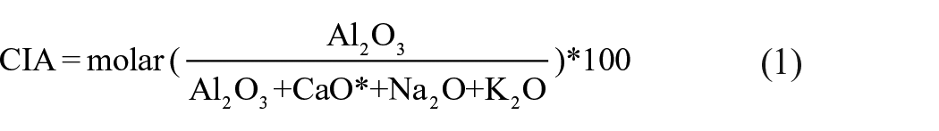
CIA = molar (\frac{{Al}_{2} O_{3}}{{Al}_{2} O_{3} {+ CaO * + Na}_{2} {O + K}_{2} O}) * 100

(1)

where CaO* represents the CaO derived from silicates rocks only (Fedo et al., 1995; Harnois, 1988; Nesbitt and Young, 1982, 1989). CaO values have been corrected to carbonate, apatite and Na₂O according to Mclennan (1993) by using the equation:

Molar CaO * = molar {CaO_10 * (P_{2} O_{5}) / 3}

(2)

We followed the assumption, if the molar (CaO) < molar (Na₂O), then the required CaO* = molar (CaO); whereas if the molar (CaO) > molar (Na₂O), then the required CaO*= molar (Na₂O).

We welcome the comments from Srivastava and Jovane (2020) in the environmental magnetic parameters part of our study. We acknowledge the typographical errors in units in relation to units in the S-ratio, χfd% and appropriate citation of Stober and Thompson (1979). However, mistakes in the units do not change our conclusions in any way.

We used geochemistry, grain size and environmental magnetic parameters to understand the climate fluctuations and glacial dynamics. Here we emphasize that the single proxy approach is not useful for any climatic studies (validation is necessary using a multi-proxy approach). We would also like to mention that Chorabari lake has a small catchment area with rapid sedimentation, and the lake is very young. Proxies therefore need some time to respond. Further, Srivastava and Jovane (2020) raises the question of the use of trace elements (Ba, Sc, V, Cr, Co, Ni, Cu, Zn, Ga, Pb, Th, Rb, U, Sr, Y, Zr and Nb). These were not included as they did not shown any significant variability and would also have no meaning in the absence of proper validation of the proxy.

Interpretations

Although the concerns of Srivastava and Jovane (2020) were raised mainly in relation to interpretation of magnetic data, Shukla et al. (2020) used multiple proxies. Their climatic interpretation were largely skewed towards interpretation of magnetic mineralogy and they largely overlooked the grain size and geochemical proxy presented in Shukla et al. (2020). We would like to highlight the fact that the approach of Shukla et al. (2020) was based on magnetic mineralogy, grain size and geochemistry. The data were correlated (except magnetic proxy data) with present-day glacial sediment response patterns at the Chorabari glacier (Kumar et al., 2016). We reasonably approached the proxy based on our long experiences in present and past studies conducted in the Chorabari valley (i.e. Bhambri et al., 2016; Dobhal et al., 2013a, b; Karakoti et al., 2017; Kumar et al., 2016; Mehta et al., 2012, 2014, 2017; Shukla et al., 2017). We have coupled the above mentioned approaches to interpret the paleo-climatic response of the Chorabari lake.

Magnetic proxy response

The environmental magnetic parameters are used to understand the distribution of ferri/antiferromagnetic minerals in the Chorabari lake profile. The environmental magnetic parameters suggest type and concentration of magnetic grains in response to climatic variability (Evans and Heller, 2003; Kumar et al., 2020a; Meena et al., 2011; Rawat et al., 2015; Srivastava et al., 2013; Verosub and Roberts, 1995). The increased χlf along with S-ratio close to negative unit value suggest the presence of low coercive minerals such as magnetite. Conversely, low χlf with a S-ratio of −0.5 or more (approaching zero), indicates the dominance of antiferromagnetic hematite (Liu et al., 2007; Thompson and Oldfield, 1986). The other parameters such as χARM and χfd% recorded the grain size dependency of magnetic minerals and enhancement in magnetic characters due to super-paramagnetic grains and single stable domain minerals (Liu et al., 2012). The high values of χlf with χARM suggest size dependent magnetite and signal warm and wet climate (Evans and Heller, 2003). Conversely, high S-ratio and low χlf are suggestive of the dominance of hematite or dilution of the magnetite signal due to enhanced input of diamagnetic and paramagnetic minerals (Evans and Heller, 2003). The significant increase of diamagnetic and paramagnetic grains are used to understand the dominance of physical weathering in a cold and dry climate. Srivastava and Jovane (2020) largely rely on the basic magnetic properties and their behaviour in non-glacial environments. We did not find any reason to neglect this proxy, although we used it to underline the inherent complexities associated with glacial sedimentary environments.

Grain-size proxy response

The sediment evacuation pattern of Chorabari glacier lake in modern (warm and wetter) climatic settings (Kumar et al., 2016) were applied to evaluate the paleoclimatic response of the region. Kumar et al. (2016) observed the dominance of medium silt to fine sand-sized particles (70–80% in the 0.0156–0.25 mm size range) without any significant seasonal variation during the ablation period of 2009–2012. The clay component is less than 1% in total suspended sediments evacuated throughout the season. The dynamic population of sediment and paleo-environmental linkages has been observed earlier (Dietze et al., 2014; Dutt et al., 2018; Kumar et al., 2020a; Weltje and Prins, 2003). In relation to grain-size proxies, we understand that dominance of sand and silt fraction represents warm and wetter conditions in the study area. It is reasonable to assume that the much lower clay fraction (<1%) represents the deposition of clay component in a low hydrodynamic environment, most likely during colder conditions with a significant reduction in the seasonal melting. We ascribed the coarser fractions to mass wasting events. Given rapid sedimentation and quick burial of glacial sediments in proglacial lake settings, we consider such grain-size proxies to provide reliable signals of past climatic variability.

Geochemical proxy response

Molar proportions of major oxides and elements were plotted with proper scientific reasoning in the ‘elemental analysis’ section of Shukla et al. (2020). We used the molar proportions of elements to quantify detailed geochemical process operating in glacial/subglacial substrates. The suggestion of Srivastava and Jovane (2020) that major oxide (Al₂O₃) and elemental (Al) molar concentrations should be plotted simultaneously could be used in future studies.

We tested the CIA values obtained from different grain-size fractions (clay, sand, coarser sand) and compared with the present day glacial suspended sediment (GSS) data set published by Kumar et al. (2016). The CIA value for GSS ranges from 54.68 to 55.18, typically showing low to moderate chemically weathered detritus, but with a slight increase in values indicating increased precipitation conditions in the catchment (Kumar et al., 2016). Chemical weathering is slower at higher altitude, because weathering is less intense for the same rate of sediment supply (Riebe et al., 2004). These CIA values are in agreement with other Himalayan glaciated basins, such as the Pindar basin (56.5) and other part of the world with granite and granodiorite lithologies, including the Alps (49-53; Eynatten et al., 2012), Southwest Iceland (45-56; Thorpe et al., 2019); and East Antarctica (57-60; Srivastava et al., 2014). By comparison, the CIA values of lake sediments show the highest value for the clay component (55-65), while coarse sand exhibits slightly lower values (51-61), indicating less alteration of rocks during deposition (Shukla et al., in review). Therefore, we used the present day CIA values of Kumar et al. (2016) as a reference for interpreting the climatic conditions in the catchment. We infer that the CIA values above 60 indicate moderate to high chemical weathering conditions at the catchment, thus validating our interpretation.

Element and oxide proxies

Along with major oxides we used elemental ratios to infer the climate-induced chemical changes in glacial sediments. For example, the Fe/Mn ratio was used to infer the paleo-redox conditions of the lake, based on the more rapidly oxidising property of iron compared to Mn, lower Mn/Fe ratios indicating higher amounts of dissolved oxygen (Mackereth, 1966; Naeher et al. 2013). Likewise Na/Al ratios were used as Na tends to be mobile in humid environments and Al tends to be conserved (Ding and Ding, 2003). Ti, Si, Al elements tend to be immobile during weathering. Ca, Na, and K are concentrated mainly in feldspars, while during weathering of granites they tend to be depleted through the process of feldspar alteration (Lee et al., 2008; Middelburg et al., 1988). We investigated these conditions with reference to specific elemental properties, enrichment factors and degree of alteration calculations. By comparison with the chemical composition of catchment rocks, the results suggest that the elemental loss for Chorabari lake sediment were mainly derived from the leachable minerals like feldspars, mica and apatite. The A-CN-K plot (where A= Al₂O₃, CN= CaO* + Na₂O and K = K₂O) applied to the lake sediments suggests that potassium is most leachable mineral shifting the pattern towards Al₂O₃ apex. This weathering reaction indicates K-metasomatism modification of sediments (e.g. Fedo et al., 1995) which follows two possible paths: either (1) due to the conversion of aluminous clay minerals (kaolinite) to illite or (2) due to the conversion of plagioclase to K- feldspars (Shukla et al., in review). Our field observations from Chorabari glacier catchment indicates the presence of large crevasses, moulins, and interconnections of supraglacial and subglacial channels promoting rapid flow through cavities of large dimensions. Mechanically disaggregated minerals (by abrasion) is preferentially leached to release different cations (especially K, Mg, Fe, and Si; Barker, 1997). Therefore the periods of high abrasion reflect little change. The low temperature and melting characteristics provide a favorable environments for mineral grains to chemically weather. Higher CIA values during the formation of clay minerals (e.g. illite) provide evidence for this process. Mg and Na are highly mobile under wetter conditions, whereas Al is less mobile, indicating differential weathering mechanisms. We used these estimates of weathering trends to explain our data accordingly.

Statistical parameters

The statistical parameters used in our previous study (Kumar et al., 2016) are presented here to demonstrate sediment variability. Grain-size statistics using the arithmetic moment method (Blott and Pye, 2001), were applied (Figure 1). Statistical formulae used in the calculation of grain-size parameters and suggested descriptive terminology are modified from Krumbein and Pettijohn (1938) and Folk and Ward (1957) is detailed in table II Blott and Pye (2001).

Figure 1.

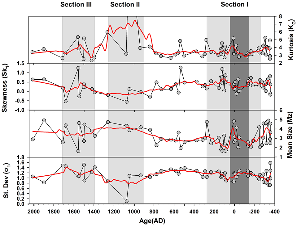
Grain-size fractions plotted against the chronology of Chorabari lake. Red line represents 2 points running average of data. The shaded part presents a proxy response in the different time periods.

Mean (M_Z) measures the mean grain size, which is compared to a glacial suspended sediment mean grain size 4.98 φ. The mean grain size of Chorabari lake has varied between 1.5-5 φ. It is representative of high (1.5 φ) to low (5 φ) hydraulic energy conditions during sedimentation in the lake. The suspended sediment mean grain size for other Himalayan sites varies within the range at Chorabari glacier: Pindari glacier (4.35 to 5.82ϕ, coarse to medium silt); Satopanth glacier (5.11 to 5.71ϕ; medium silt); Dokriani glacier (4.05 to 6ϕ; coarse to fine silt); and Gangotri glacier (4.7 to 6ϕ; coarse to medium silt) (Haritashya et al., 2010; Kumar et al., 2016; Pandey et al., 2002; Thayyen et al., 1999).

Standard deviation (sorting) (σ₁) is used to evaluate sorting with respect to different grain-size fractions deposited in the lake. The mean value for glacial suspended sediment evacuation was 1.61 φ. However, the lake sediment sorting varied between 0.2 and 1.6 φ. The average values for sorting varies between 1.2–2.44 φ for Pindari, Satopanth, Dokriani, Gangotri and Chorabari glacier systems in the Himalayas (Haritashya et al., 2010; Kumar et al., 2016; Pandey et al., 2002; Thayyen et al., 1999). These values indicate the poorly sorted sediments evacuating from present-day warm and humid climatic settings.

Skewness (Sk₁) characterizes the symmetry of the grain-size distribution and is interpreted in terms of the energy conditions during the deposition. The Chorabari glacial suspended sediments evacuation pattern were characterized by, negatively skewed values (− 0.11 – −0.017), indicating the presence of relatively finer grain sizes in glacial melt water (Kumar et al., 2016). The coarsely skewed to nearly symmetrical pattern suggests the evacuation of suspended sediments in high energy environments (Folk, 1968). Other Himalayan basins have chaotic skewness values, such as Pindari glacier (−0.31–1.14), Satopanth glacier (0.10–0.51), Gangotri glacier (−0.17–0.02) (Haritashya et al., 2010; Pandey et al., 2002). The skewness values for Chorabari lake sediments range from −0.5 to 1.25 suggesting coarsely skewed to very fine skewed nature. The chaotic values of skewness suggest variability in the Himalayan glacier dynamics.

Kurtosis (K_G), enables assessment of the degree of peakedness of grain-size distributions. Glacial suspended sediments have a mesokurtic distribution (kurtosis 1.02) whereas values for the Chorabari lake sediments range from 2.5 to 9, suggesting leptokurtic distributions. The kurtosis values for different glacier systems in the Himalayas range from 0.9 to 1.36 in the Pindari, Satopanth, Dokriani, Gangotri and Chorabari glacier systems (Haritashya et al., 2010; Kumar et al., 2016; Pandey et al., 2002; Thayyen et al., 1999). The dominance of platykurtic to mesokurtic nature of the glacial suspended sediments exhibits mixing two populations in the subequal amount. However, the leptokurtic nature of lake sediments refers to the continuous addition of finer or coarser materials during deposition (Avramidis et al., 2013).

Bivariate plots

The grain-size proxy has been tested for its responsiveness in different climatic settings through bivariate plots (Figure 2a–c). The bivariate plots of mean size-standard deviation, skewness-standard deviation and kurtosis suggest distinct populations characteristic of sediments, on the one hand, warm and humid conditions and, on the other hand, cold and dry periods (Shukla et al., 2020). The mixing of a few data points can be observed within the periods characterized as cold and dry because distinct warm pulses were also present. We further verified the depositional environment of Chorabari lake with scanning electron microscopy (SEM). This technique identifies the surface textural features of mineral grains, which preserve the imprints of a particular environment. The detailed methodology is explained in Kumar et al. (2011). The grain outlines of section I represents the less sharp edges, broken surfaces, adhered particles, straight and arcuate steps, mineral precipitation, and surface alteration (Figure 3a, b). It represents the sediment has suffered hot-humid to a cold and dry environment. However, the section II grain morphology includes conchoidal fractures (>100 µm) size (Figure 3c, d): arcuate grooves and curved conchoidal fractures are commonly observed in quartz grains of glacial origin (Krinsley and Donahue, 1968). The grain morphology observed in section II suggests grain transport by meltwater streams (Whalley and Krinsley, 1974). The ragged and fleecy edges of rounded grains in section III, which represent grain coatings of flaky mica (Figure 3e, f) indicate physical weathering and clay formation under cold conditions.

Figure 2.

Bivariate plots of grain-size statistics show three distinct populations for Chorabari lake sediments. (a) mean size vs standard deviation; (b) Skewness vs Kurtosis; (c) skewness vs standard deviation. Shaded part in (b, c) highlights sediment deposition at low lake water levels under cold climatic conditions when the unsorted sediments have increased.

Figure 3.

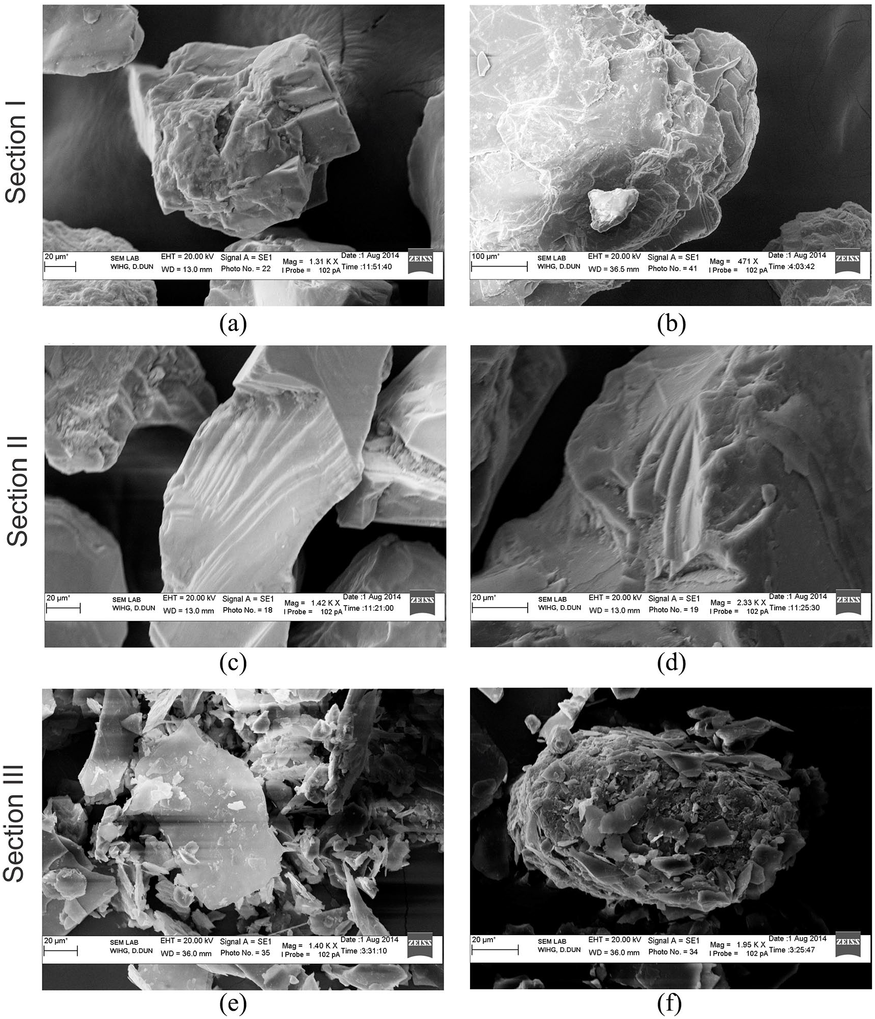
SEM images of lake-sediment grains from three distinct populations. (a, b) presents less sharp edges, broken surfaces, adhered particles, straight and arcuate steps, mineral precipitation and surface alteration; (c, d) presents sharp conchoidal fractures (>100 µm) on quartz grains; (e, f) presents rounded grains with flaky mineral coatings indicating more intense weathering and clay formation during cold conditions.

Loss on ignition (LOI) proxy

This proxy can be used to infer the organic, carbonate and/or minerogenic clastic material content in the lake sediments (cf. Cato, 1977; Sekar, 2000; Wunnemann et al., 2008). We used a sequential weighted LOI method with samples first dried at 105ºC, then ignited in a furnace at 550ºC and 950ºC, respectively (Battarbee et al., 2002; Nesje et al., 2004).

We measured the total organic content (TOC) of the samples through the Isotope Ratio Mass Spectrometer (IRMS) facility at Wadia Institute of Himalayan Geology, Dehradun. We found a good correlation between LOI 550ºC and TOC data (R² = 0.73) which has presented a firm basis for using it as a representative of organic carbon content in the Chorabari lake region (Figure 4).

Figure 4.

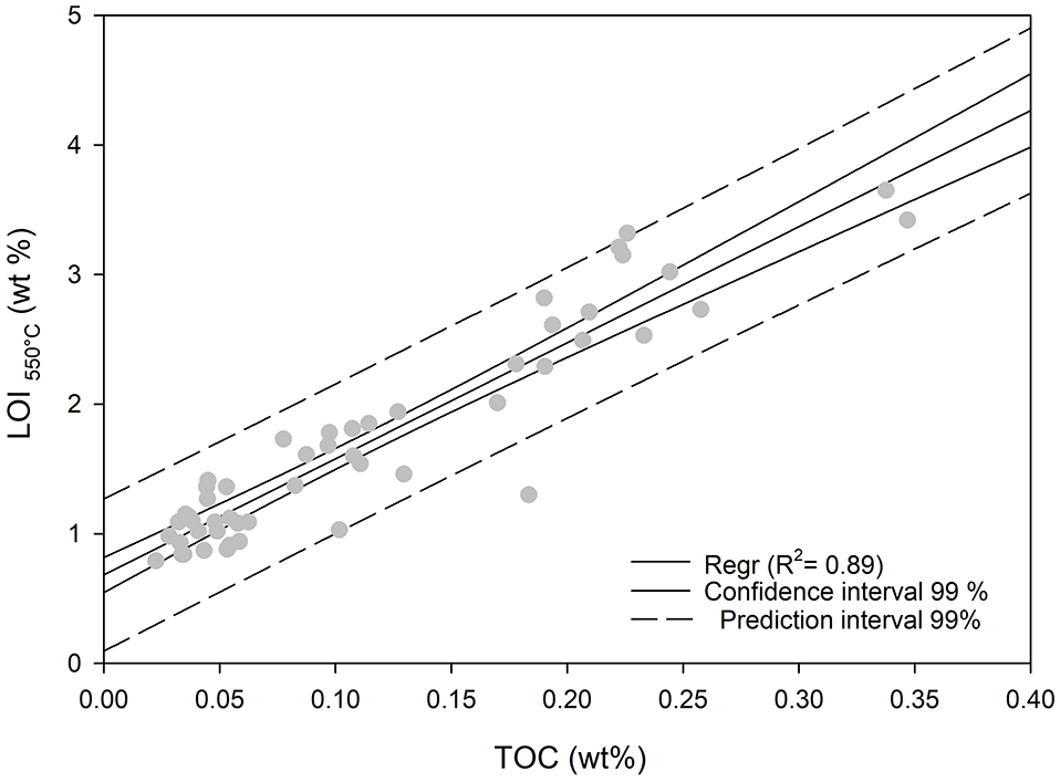
Bivariate plot of Total Organic Carbon (TOC) and Loss on Ignition (LOI) supporting the use of LOI-550ºC as a suitable proxy for organic carbon deposition at Chorabari Lake.

The response of proxies like CIA, Al%, Ti%, Fe/Mn, K₂O, Al₂O₃, LOI and Fe₂O₃ and high Na₂O, Na/Al and Ca/Mg, and magnetic mineralogy were behaving in almost an inverse way in the Mediaeval Warm Period (MWP) compared to the Little Ice Age (LIA). However, during the LIA, we observed a mixed response due to short pulses of humid climate, and there is a lag in the response of the geochemical proxies (Na, K, P and Ca) affected by clay deposition.

OSL chronology and lake sediment accumulation rate (SAR)

Srivastava and Jovane (2020) cast doubt over the reliability of our OSL ages. We used the well-established SAR protocol to estimate the paleodoses (Murray and Wintle, 2000). Briefly, the equivalent dose (paleodose) represents the average or representative value of a radiation dose accumulated in a sample due to the decay of naturally occuring radionuclides since they were last exposed to sunlight (Aitken, 1998). We obtained the equivalent doses using medium-size aliquots with an average of 400–500 quartz grains. Thereafter, the total standard deviation of each sample was calculated, which includes both the natural variation between grains and sampling errors. The final ages were calculated using the minimum age model (20%) detailed in Ray and Srivastava (2010).

Numerous studies are available worldwide on reconstructing spatial and temporal changes in lacustrine sedimentary sequences through OSL dating, for example from the Tibetan Plateau (Fan et al., 2010; Lu et al., 2007); Western China (Yang et al., 2006); Northern China (Long et al., 2011; Zhang et al., 2012); Central Himalaya (Bali et al., 2017; Juyal et al., 2009; Srivastava et al., 2013); Central Tibet (Pan et al., 2012); Antarctica (Doran et al., 1999); and Siberia (Forman et al., 2007; Juschus et al., 2007; Moska et al., 2008). The suggestion of Srivastava and Jovane (2020) of alternate dating methods (e.g. radiocarbon) is not useful, as the sediments suffer from low organic content. Considering the recent developments in the OSL dating technique (e.g. Rhodes, 2011; Roberts, 2008) a step-change improvement in the accuracy, precision has been documented. This has arguably improved confidence in using quartz as a dosimeter and first mineral of choice for OSL dating (cf. Murray and Olley, 2002). Therefore, in the absence of other datable material, we find this technique unexceptionable for high energy settings with low organic productivity. In Garhwal Himalaya, moreover, at the Garbyang and Malari landslide-dammed lakes, the stratigraphy was established using OSL chronology and used to discuss the monsoon variability in the late Pleistocene and Holocene (Juyal et al., 2004; Srivastava et al., 2013). Furthermore, in these studies, ¹⁴C dating was discarded because of random age patterns and age overestimation. Both studies suggested a ‘hard water effect’ and contamination by older carbon. Hence, the claims that the OSL technique is unreliable are vague.

Srivastava and Jovane (2020) have also criticized our stratigraphy and challenge our sediment accumulation rate (SAR). However, they compare our high cool-climate rates with those found in warm-humid climates and take no account of the sedimentary sequence at Chorabari lake, which bears witness to several high-energy events. Thus, an average sedimentation rate has little meaning at our site. A constant SAR between two ages suggesting constant paleo-environmental conditions which are inapplicable where rates of erosion in the headwaters and sediment transfer in the basin are variable. Such variations are apparent in our stratigraphy, which shows beds of clay and silt and thin beds of coarse sand. This suggests that overall the climate was cold but there were a few phases of different hydrologic conditions due to enhanced glacial melting.

Further discussion

The major concerns of Srivastava and Jovane (2020) involve our interpretation of magnetic mineralogy, chronology and sediment accumulation rate. They largely ignore the specific physical conditions of the Himalayan glacial sedimentary environment, where grain maturity and magnetic properties are not as developed as in glacier-free catchments.

Their comment on the presence of greigite and bacterial (ferrimagnetic) magnetite as an influence on authigenic magnetic minerals has not been validated in any Himalayan glacierized basin. Authigenic greigite and bacterial magnetite are produced during the eutrophication of lakes leading to dysaerobic conditions with high productivity and organic matter (Muller, 1996; Evans and Heller, 2003). We have no evidence of a bacterial magnetite signature from the values of the magnetic grain-size indicator (χARM/χlf) from Chorabari lake. In connection with authigenic magnetic minerals, physical weathering through frost and thawing supply mostly immature sediments (Kumar et al., 2016; Srivastava et al., 2017). The duration of sedimentation in the lake was not long enough to permit diagenetic processes and authigenic mineralization. Srivastava and Jovane (2020) suggest we supplied insufficient information about the dissolution of magnetite during slow deposition rates, the preservation of the magnetite during rapid sedimentation, and the relatively high/low S-ratio. But as the present lake is not a eutrophic lake, such a discussion is unnecessary. Although, the S-ratio registers the presence of ferrimagnetic/antiferromagnetic minerals (Liu et al., 2007; Thompson and Oldfield, 1986), the concentration of these minerals in the lake is diluted by the enhanced input of paramagnetic and diamagnetic minerals that we tried to relate with the climate change (cf. Rawat et al., 2015; Srivastava et al., 2013; 2017).

Srivastava and Jovane (2020) have misinterpreted our statement that ‘in periods of climatic transition, the supply of minerogenic material to lakes is reduced and the sediment with a lower organic content were deposited. A slow deposition rate could also lead to magnetite dissolution, resulting in a low magnetic concentration and high S-ratio. Conversely, during periods of glacial retreat, the minerogenic sedimentation rate increases and magnetite is preserved in the sediments because of rapid burial, which results in a high magnetic concentration and low S-ratio’. We explicitly mentioned the assumptions and interpretive framework of magnetic data with a source of error and caution against generalized interpretations. Since we have not validated the magnetic proxies for glacial suspended sediment release, therefore, the magnetic data interpretation presented could be treated as tentative. Srivastava and Jovane (2020) himself found it difficult to interpret the climate signals due to inherent complexities in present settings.

Section I (260 BCE and 270 CE)

The climatic signals in section I were interpreted as: “moderate to low CIA, LOI-550°C, Fe₂O₃ with high to low Fe/Mn, Ca/Mg, Na/Al, Na₂O%, SiO₂%, K₂O% and Al₂O₃% values showing the transition of arid/warmer climate to cold and dry conditions at ~0–200 CE. Low Al₂O₃, Fe₂O₃, Ti, Fe/Mn ratios and high Na₂O, Ca/Mg, Na/Al ratios suggest poor chemical weathering under deprived precipitation and deteriorating climatic condition.” In addition, the grain-size proxy, with mean grain sizes of 2–4 φ, poorly to well-sorted sediments and, positively skewed, leptokurtic grain-size distributions, suggest oscillating climatic conditions from cold to dry climatic settings. The overall grain size data suggests the dominance of sand-sized grains with occasional occurrence of clay. When grain size is fine sand with low χlf and χARM and high S-ratio, the dominance of antiferromagnetic minerals or low presence of ferrimagnetic minerals is suggested. At ~260 BCE to ~170 BCE, χlf and χARM are high where the mean grain size is sandy and χfd% and the S-ratio suggest the presence of SSD minerals. At 170 BCE to ~40 CE, higher sand concentrations, low χlf, low χARM and other parameters suggest low concentrations of magnetic grains or MD magnetic minerals. At ~40 to ~280 CE, low χlf and χARM suggest a low concentration of magnetic grains and, conversely, high χfd% and low S-ratio suggest the presence of ferrimagnetic minerals. At this point, the overall response of the non-magnetic proxies indicates fluctuating climatic conditions (cool and dry to hot and humid climate) as concluded by Shukla et al. (2020).

Section II (~900–1260 CE):

We interpreted this section as “moderate to high CIA values, decreasing trend from high to low Na₂O, Na/ Al, Ca/Mg, and SiO₂, and increasing trends from low to high K₂O, Al₂O₃, and Fe/Mn ratios. It suggests high chemical weathering in the catchment and warm/humid conditions at the Chorabari lake.” The statistical parameters for grain-size proxy in this section presents the mean grain size range ~4 φ (similar to present-day mean grain size evacuating from different glacierized basins of the Himalaya). Since the standard deviation is also low, moderate to well-sorted conditions are suggested, and negatively skewed, very leptokurtic grain size fractions also indicate rapidly changing hydrodynamic conditions. At ~900 to ~1250 CE, low χlf and χARM suggest a poor concentration of ferrimagnetic minerals. However, grain size suggests the dominance of the silt fraction. Collectively, the magnetic grains are of silt size and magnetic signals were diluted due to a higher input of paramagnetic and diamagnetic minerals (high concentration of quartz and feldspars minerals) in the bulk sediment from erosion in the catchment. The kurtosis (Figure 1) values suggest relatively strong hydrodynamic conditions in the catchment indicate the erosion due to the enhanced melting of Chorabari glacier in warm climate. Furthermore, the clay component of this zone is nearly 1%, similar to that of the present-day suspended load (Kumar et al., 2016) (hot and humid climate). Therefore, it is reasonable to conclude that the period had a similar climatic condition to the present day.

Section III (~1370–1720 CE)

The period ~1370–1720 CE is characterized by “low CIA, Al%, Ti%, Fe/Mn, K₂O, Al₂O₃, LOI-550°C, Fe₂O₃ values and high Na₂O, Na/Al, Ca/Mg values, indicating low weathering under cold climatic conditions with low organic productivity. However, at ~1500 and 1550 CE, a sudden rise in these values denotes stronger hydrodynamics and moderate weathering conditions.” The grain size proxy also suggests variation in the sand to clay fractions, suggesting the switching between hot-humid to cold and dry climatic conditions. It is important to notice that freeze-thaw events are also characteristic in the basin, which enhances physical weathering and supply clastic sediments in the basin. An increase in the SiO₂ molar fraction and alternate bands of Al molar fraction support the notion of increased clastic content. However, the Na, which has a tendency to be dissolved in water, suggests the availability of glacial meltwater. The environmental magnetic parameters, χlf and χARM, are relatively low in this section. And the S-ratio indicates low concentrations of ferrimagnetic magnetic grains. Therefore, it is likely that this period witnessed increased clastic input under cold/dry catchment conditions coupled with intervening humid pulses generating high glacial meltwater discharge. Statistical parameters of grain size also support the fluctuating climatic conditions with high standard deviation. Positive to negatively skewed leptokurtic behaviour strengthens our conclusions for the period 1370–1720 CE (corresponding to the LIA), which shows a distinct event with intermittent warming and cooling episodes as evidenced in other parts of the Himalaya and elsewhere.

Regional correlations

The concern of Srivastava and Jovane (2020) about the pattern of glaciation in precipitation-deprived regions presents their unawareness of the sensitivity of glaciers to the climate system. We do not agree with Srivastava and Jovane (2020) over the interplay of precipitation and temperature in driving the glaciation mechanism over the central Himalaya. There are numerous studies on the pattern of mountain glaciation and its sensitivity to changes in precipitation and temperature (Kumar et al., 2020b; Mackintosh et al. 2017; Owen et al. 2006; Pratt-Sitaula et al. 2011; Roe et al. 2017; Shukla et al., 2018; Zech et al. 2009). Recent studies have shown that the precipitation-dominated regions (mean annual precipitation >1000 mm) are very sensitive towards temperature changes (Shukla et al., 2018; Zech et al., 2009). However, the precipitation-deprived regions (mean annual precipitation <500 mm) preserve sensitivity towards changes in precipitation (Kumar et al., 2020b, 2020c). In our recent study (Kumar et al., 2020b) we presented a close correspondence between mass balance sensitivity and precipitation changes in a precipitation-deprived glacial valley, where mass gain occurred during cooler climatic conditions was preserved for longer periods than precipitation-dominated valleys (Kumar et al., 2020b; Shukla et al., 2018). The glacial condition in the catchment was likely sustained by the presence of snow cover for longer duration (Kumar et al., 2020b; Pratt-Sitaula et al. 2011; Zech et al. 2009). Year-by-year deposition of fresh snow enhances the positive feedback of snow albedo, and this changes the atmospheric circulation leading to the sustaining of the glacial conditions (Dobhal et al., 2013a,b). The concept of cool summers combined with mild winters, followed by temperature-moisture feedback leading to enhanced precipitation and reduced snowmelt, provides a sound explanation for the waxing and waning of the glaciers at high altitudes coupled with insolation-induced variability (Dobhal et al., 2013a,b). Our estimates from Chorabari lake suggest that the periods of monsoon enhancement is widely correlated with the response of precipitation-deprived regions.

Conclusions

(1). The references cited in our original paper (Shukla et al., 2020) are sufficient and appropriate.

(2). The comments of Srivastava and Jovane (2020) relating to sediment accumulate rate have no meaning in the high-energy (glacial) catchment of Chorabari lake. The chronological basis of our stratigraphy is well established by well-tested OSL technique and age models.

(3). Climatic interpretation of our lake sediment stratigraphy based on magnetic data alone is not sufficient. Magnetic data need supporting proxy records for validation before proper data interpretation.

(4). Data based on grain-size and geochemistry strengthens further the interpretations presented in Shukla et al. (2020) in which we conclude.

(5). None of the evidence presented by Srivastava and Jovane (2020) requires any revision of conclusions reached by Shukla et al. (2020) study.

Footnotes

Acknowledgements

We would like to thank for highlighting the other aspects of our research. Looking deep into their suggestions and ultimately reassessing our data gives us more confidence in standing by our results. Nevertheless, the discussion paper would benefit a wider audience working on climate using proxy data. We are thankful to Prof. John A. Matthews, Editor, The Holocene, for inviting us to write a reply. The authors sincerely thank Director, Wadia Institute of Himalayan Geology (WIHG), Dehradun for providing necessary facilities to carry out this work.

Funding

The author(s) received no financial support for the research, authorship, and/or publication of this article.

ORCID iDs

Tanuj Shukla

Manish Mehta

References

Aitken

(1998) An Introduction to Optical Dating. London: Academic Press.

Avramidis

Samiotis

Kalimani

et al. (2013) Sediment characteristics and water physicochemical parameters of the Lysimachia Lake, Western Greece. Environmental Earth Sciences 70(1): 383–392.

Bali

Khan

Sangode

, et al. (2017) Mid-to late Holocene climate response from the Triloknathpalaeolake, Lahaul Himalaya based on multiproxy data. Geomorphology 284: 206–219.

Barker

(1997) Biogeochemical weathering of silicate minerals. Geochemistry: Interactions between Microbes and Minerals 35: 391–428.

Battarbee

Grytnes

Thompson

, et al. (2002) Comparing palaeolimnological and instrumental evidence of climate change for remote mountain lakes over the last 200 years. Journal of Paleolimnology 28: 161–179.

Bhambri

Mehta

Dobhal

et al. (2016) Devastation in the Kedarnath (Mandakini) valley, Garhwal Himalaya, during 16–17 June 2013: A remote sensing and ground-based assessment. Natural Hazards 80(3): 1801–1822.

Bhutiyani

(2000) Sediment load characteristics of a proglacial stream of Siachen Glacier and the erosion rate in Nubra valley in the Karakoram Himalayas, India. Journal of Hydrology 227(1–4): 84–92.

Blott

Pye

(2001) GRADISTAT: A grain size distribution and statistics package for the analysis of unconsolidated sediments. Earth surface processes and Landforms 26(11): 1237–1248.

Cato

(1977) Recent sedimentological and geochemical conditions and pollution problems in two marine areas in south-western Sweden. Striae 6: 15

10.

Cook

Swift

(2012) Subglacial basins: Their origin and importance in glacial systems and landscapes. Earth-Science Reviews 115(4): 332–372.

11.

Curry

Ballantyne

(1999) Paraglacial modification of glacigenic sediment. GeografiskaAnnaler: Series A, Physical Geography 81(3): 409–419.

12.

Dietze

Maussion

Ahlborn

, et al. (2014). Sediment transport processes across the Tibetan Plateau inferred from robust grain-size end members in lake sediments. Climate of the Past 10(1): 91–106.

13.

Ding

(2003) Chemical weathering history of the southern Tajikistan loess and paloclimate implications. Science in China Series D: Earth Sciences 46(10): 1012–1021.

14.

Dobhal

Gupta

Manish

, et al. (2013a) Kedarnath disaster: Facts and plausible causes. Current Science 105(2): 171–174.

15.

Dobhal

Mehta

Srivastava

(2013b) Influence of debris cover on terminus retreat and mass changes of Chorabari Glacier, Garhwal region, central Himalaya, India. Journal of Glaciology 59(217): 961–971.

16.

Doran

Berger

Lyons

(1999) Dating quaternary lacustrine sediments in the McMurdo Dry Valleys, Antarctica. Palaeogeography, Palaeoclimatology, Palaeoecology 147(3–4): 223–239.

17.

Dutt

Gupta

Wünnemann

, et al. (2018) A long arid interlude in the Indian summer monsoon during∼ 4,350 to 3,450 cal. yr BP contemporaneous to displacement of the Indus valley civilization. Quaternary International 482: 83–92.

18.

Evans

DJA

Phillips

Hiemstra

, et al. (2006) Subglacial till: formation, sedimentary characteristics and classification. Earth-Science Reviews 78(1–2): 115–176.

19.

Evans

Heller

(2003) Environmental Magnetism: Principles and Applications of Enviromagnetics. Elsevier, 86, p. 299.

20.

Fan

Lai

Long

, et al. (2010) OSL chronology for lacustrine sediments recording high stands of Gahai Lake in Qaidam Basin, northeastern Qinghai–Tibetan Plateau. Quaternary Geochronology 5(2–3): 223–227.

21.

Fedo

Wayne Nesbitt

Young

(1995) Unraveling the effects of potassium metasomatism in sedimentary rocks and paleosols, with implications for paleoweathering conditions and provenance. Geology 23(10): 921–924.

22.

Folk

(1968) Petrology of Sedimentary Rocks. Austin, TX: Hemphill Publishing Co.

23.

Folk

Ward

(1957) Brazos River bar [Texas]; a study in the significance of grain size parameters. Journal of Sedimentary Research 27(1): 3–26.

24.

Forman

Pierson

Gomez

, et al. (2007) Luminescence geochronology for sediments from Lake El’gygytgyn, northeast Siberia, Russia: Constraining the timing of paleoenvironmental events for the past 200 ka. Journal of Paleolimnology 37(1): 77–88.

25.

Geiss

Banerjee

(1997) A multi-parameter rock magnetic record of the last glacial–interglacial paleoclimate from south-central Illinois, USA. Earth and Planetary Science Letters 152(1–4): 203–216.

26.

Gupta

Anderson

Overpeck

(2003) Abrupt changes in the Asian southwest monsoon during the Holocene and their links to the North Atlantic Ocean. Nature 421(6921): 354–357.

27.

Gupta

Das

Anderson

(2005) Solar influence on the Indian summer monsoon during the Holocene. Geophysical Research Letters 32(17).

28.

Haldorsen

(1981) Grain-size distribution of subglacial till and its relation to glacials crushing and abrasion. Boreas 10(1): 91–105.

29.

Hambrey

Ehrmann

(2004) Modification of sediment characteristics during glacial transport in high-alpine catchments: Mount Cook area, New Zealand. Boreas 33(4): 300–318.

30.

Hammer

Smith

(1983) Sediment production and transport in a proglacial stream: Hilda Glacier, Alberta, Canada. Boreas 12(2): 91–106.

31.

Haritashya

Kumar

Singh

(2010) Particle size characteristics of suspended sediment transported in meltwater from the Gangotri Glacier, central Himalaya—An indicator of subglacial sediment evacuation. Geomorphology 122(1–2): 140–152.

32.

Haritashya

Singh

Kumar

, et al. (2006) Suspended sediment from the Gangotri Glacier: Quantification, variability and associations with discharge and air temperature. Journal of Hydrology 321(1–4): 116–130.

33.

Harnois

(1988) The CIW index: A new chemical index of weathering. Sedimentary Geology 55(3): 319–322.

34.

Juschus

Preusser

Melles

, et al. (2007) Applying SAR-IRSL methodology for dating fine-grained sediments from Lake El’gygytgyn, north-eastern Siberia. Quaternary Geochronology 2(1–4): 187–194.

35.

Juyal

Pant

Basavaiah

, et al. (2004) Climate and seismicity in the higher Central Himalaya during 20–10 ka: evidence from the Garbayang basin, Uttaranchal, India. Palaeogeography, Palaeoclimatology, Palaeoecology 213(3–4): 315–330.

36.

Juyal

Pant

Basavaiah

, et al. (2009) Reconstruction of Last Glacial to early Holocene monsoon variability from relict lake sediments of the Higher Central Himalaya, Uttrakhand, India. Journal of Asian Earth Sciences 34(3): 437–449.

37.

Karakoti

Kesarwani

Mehta

, et al. (2017) Modelling of meteorological parameters for the Chorabari Glacier valley, Central Himalaya, India. Current Science 112(7): 1553.

38.

Kirkbride

(1995) Processes of transportation. Modern Glacial Environments: Processes, Dynamics and Sediments 1: 261–292.

39.

Krinsley

Donahue

(1968) Environmental interpretation of sand grain surface textures by electron microscopy. Geological Society of America Bulletin 79(6): 743–748.

40.

Krumbein

Pettijohn

(1938) Manual of Sedimentary Petrography. New York: Appleton-Century-Crofts, Inc.

41.

Kumar

Dutt

Saraswat

Gupta

, et al. (2020a) A late Pleistocene sedimentation in the Indus Fan, Arabian Sea, IODP Site U1457. Geological Magazine 157(6): 920–928.

42.

Kumar

Gokhale

Shukla

, et al. (2016) Hydroclimatic influence on particle size distribution of suspended sediments evacuated from debris-covered Chorabari Glacier, upper Mandakini catchment, central Himalaya. Geomorphology 265: 45–67.

43.

Kumar

Bharti

Gusain

, et al. (2011) Scanning electron microscopy of Streptomyces without use of any chemical fixatives. Scanning 33(6): 446–449.

44.

Kumar

Shukla

Mishra

, et al. (2020b) Chronology and climate sensitivity of the post-LGM glaciation in the Dunagiri valley, Dhauliganga basin, Central Himalaya, India. Boreas. 49(3): 594–614 DOI: 10.1111/bor.12440.

45.

Kumar

Shukla

Mehta

et al. (2020c) Glacier changes and associated climate drivers for the last three decades, Nanda Devi region, Central Himalaya, India. Quaternary International. DOI: 10.1016/j.quaint.2020.06.017.

46.

Lee

Kim

Baik

(2008) Chemical weathering of granite under acid rainfall environment, Korea. Environmental Geology 55(4): 853–862.

47.

Long

Lai

Wang

Zhang

(2011) A combined luminescence and radiocarbon dating study of Holocene lacustrine sediments from arid northern China. Quaternary Geochronology 6(1): 1–9.

48.

Liu

Roberts

Larrasoana

, et al. (2012) Environmental magnetism: principles and applications. Reviews of Geophysics 50(4): RG4002, 1–50.

49.

Liu

Roberts

Torrent

, et al. (2007) What do the HIRM and S-ratio really measure in environmental magnetism? Geochemistry, Geophysics, Geosystems 8(9): Q09011.

50.

Wang

Wintle

(2007) A new OSL chronology for dust accumulation in the last 130,000 yr for the Chinese Loess Plateau. Quaternary Research 67(1): 152–160.

51.

Mackereth

FJH

(1966) Some chemical observations on post-glacial lake sediments. Philosophical Transactions of the Royal Society of London. Series B, Biological Science 250: 165–213.

52.

Mackintosh

Anderson

Lorrey

et al. (2017) Regional cooling caused recent New Zealand glacier advances in a period of global warming. Nature Communications 8(1): 1–13.

53.

McLennan

(1993) Weathering and global denudation. The Journal of Geology 101(2): 295–303.

54.

Meena

Maiti

Shrivastava

(2011) Discrimination between anthropogenic (pollution) and lithogenic magnetic fraction in urban soils (Delhi, India) using environmental magnetism. Journal of Applied Geophysics 73(2): 121–129.

55.

Mehta

Dobhal

Kesarwani

, et al. (2014) Monitoring of glacier changes and response time in Chorabari Glacier, Central Himalaya, Garhwal, India. Current Science 107(2): 281–289.

56.

Mehta

Majeed

Dobhal

, et al. (2012) Geomorphological evidences of post-LGM glacial advancements in the Himalaya: A study from Chorabari Glacier, Garhwal Himalaya, India. Journal of Earth System Science 121(1): 149–163.

57.

Mehta

Shukla

Bhambri

, et al. (2017) Terrain changes, caused by the 15–17 June 2013 heavy rainfall in the Garhwal Himalaya, India: A case study of Alaknanda and Mandakini basins. Geomorphology 284: 53–71.

58.

Menzies

van der Meer

Rose

(2006) Till as a glacial “tectomict”, its internal architecture, and the development of a “typing” method for till differentiation. Geomorphology 75(1–2): 172–200.

59.

Middelburg

Van der Weijden

Woittiez

(1988) Chemical processes affecting the mobility of major, minor and trace elements during weathering of granitic rocks. Chemical Geology 68(3–4): 253–273.

60.

Moska

Poręba

Bluszcz

Wiszniowska

(2008) Combined IRSL/OSL dating on fine grains from Lake Baikal sediments. Geochronometria 31(1): 39–43.

61.

Müller

TLB

(1996) Microbially mediated iron mineral transformations: A case study in Lake Greifen, Switzerland. Doctoral Dissertation. Zurich: ETH Zurich.

62.

Murray

Olley

(2002) Precision and accuracy in the optically stimulated luminescence dating of sedimentary quartz: a status review. Geochronometria 21(1): 1–16.

63.

Murray

Wintle

(2000) Luminescence dating of quartz using an improved single-aliquot regenerative-dose protocol. Radiation Measurements 32(1): 57–73.

64.

Naeher

Gili

North

, et al. (2013) Tracing bottom water ox-ygenation with sedimentary Mn/Fe ratios in Lake Zurich, Schwitzerland. Chemical Geology 352: 125–133.

65.

Nesje

Dahl

Lie

(2004) Holocene millennial-scale summer temperature variability inferred from sediment parameters in a non-glacial mountain lake, Danntjørn, Jotunheimen, central southern Norway. Quaternary Science Reviews 23(2004): 2183–2205.

66.

Nesbitt

Young

(1982) Early Proterozoic climates and plate motions inferred from major element chemistry of lutites. Nature 299(5885): 715–717.

67.

Nesbitt

Young

(1989) Formation and diagenesis of weathering profiles. The Journal of Geology 97(2): 129–147.

68.

Norrish

Hutton

(1969) An accurate X-ray spectrographic method for the analysis of a wide range of geological samples. Geochimica et Cosmochimica Acta 33: 431–453.

69.

Owen

Derbyshire

Scott

(2003) Contemporary sediment production and transfer in high-altitude glaciers. Sedimentary Geology 155(1–2): 13–36.

70.

Owen

Finkel

Haizhou

et al. (2006) Late Quaternary landscape evolution in the Kunlun Mountains and Qaidam Basin, Northern Tibet: A framework for examining the links between glaciation, lake level changes and alluvial fan formation. Quaternary International 154: 73–86.

71.

Pan

Jiang

, et al. (2012) Holocene lake-level changes of Linggo Co in central Tibet. Quaternary Geochronology 10: 117–122.

72.

Pandey

Singh

Hasnain

(2002) Grain-size distribution, morphoscopy and elemental chemistry of suspended sediments of Pindari Glacier, Kumaon Himalaya, India. Hydrological Sciences Journal 47(2): 213–226.

73.

Potts

(1987) X-ray fluorescence analysis: Principles and practice of wavelength dispersive spectrometry. In: Potts

(ed.) A Handbook of Silicate Rock Analysis. Dordrecht: Springer, pp. 226–285.

74.

Pratt-Sitaula

Burbank

Heimsath

et al. (2011) Topographic control of asynchronous glacial advances: A case study from Annapurna, Nepal. Geophysical Research Letters 38(24): L24502.

75.

Purohit

Sanyal

Roy

, et al. (2010) 13C enrichment in the Palaeoproterozoic carbonate rocks of the Aravalli Supergroup, northwest India: Influence of depositional environment. Gondwana Research 18 (2–3): 538–546.

76.

Rawat

Gupta

Srivastava

(2015) A 13,000 year record of environmental magnetic variations in the lake and peat deposits from the Chandra valley, Lahaul: Implications to Holocene monsoonal variability in the NW Himalaya. Palaeogeography, Palaeoclimatology, Palaeoecology 440: 116–127.

77.

Ray

Srivastava

(2010) Widespread aggradation in the mountainous catchment of the Alaknanda–Ganga River System: Timescales and implications to Hinterland–foreland relationships. Quaternary Science Reviews 29(17–18): 2238–2260.

78.

Rhodes

(2011) Optically stimulated luminescence dating of sediments over the past 200,000 years. Annual Review of Earth and Planetary Sciences 39: 461–488.

79.

Riebe

Kirchner

Finkel

(2004) Erosional and climatic effects on long-term chemical weathering rates in granitic landscapes spanning diverse climate regimes. Earth and Planetary Science Letters 224(3–4): 547–562.

80.

Roberts

(2008) The development and application of luminescence dating to loess deposits: a perspective on the past, present and future. Boreas 37(4): 483–507.

81.

Roe

Baker

Herla

(2017) Centennial glacier retreat as categorical evidence of regional climate change. Nature Geoscience 10(2): 95–99.

82.

Saini

Mukherjee

Rathi

(2002) Trace element estimation in soils: An appraisal of ED-XRF technique using group analysis scheme. Journal of Trace and Microprobe Techniques 20(4): 539–551.

83.

Sekar

(2000) Interpretation of past climatic changes around Tsokar Lake, Ladakh for the last 33 Ka on the basis of chemical data. Palaeobotanist 49: 519–527.

84.

Shukla

Mehta

Dobhal

, et al. (2020) Late-Holocene climate response and glacial fluctuations revealed by the sediment record of the monsoon-dominated Chorabari Lake, Central Himalaya. The Holocene 30(7): 953–965.

85.

Shukla

Mehta

Jaiswal

, et al. (2018) Late Quaternary glaciation history of monsoon-dominated Dingad basin, central Himalaya, India. Quaternary Science Reviews 181: 43–64.

86.

Shukla

Mehta

Kumar

, et al. (2017) Application of the Schmidt-hammer with relative-age dating of moraine boulders-a case study from Mandakini River valley, central Himalaya, India. Himalayan Geology 38(2): 184–192.

87.

Shukla

Sundriyal

Stachnik

, et al. (2018) Carbonate and silicate weathering in glacial environments and its relation to atmospheric CO₂ cycling in the Himalaya. Annals of Glaciology 59(77): 159–170.

88.

Srivastava

Jovane

(2020) Misinterpreting proxy data for paleoclimate signals: A comment on Shukla et al. 2020. The Holocene. DOI: 10.1177/0959683620941165.

89.

Srivastava

Agnihotri

Sharma

, et al. (2017) 8000-year monsoonal record from Himalaya revealing reinforcement of tropical and global climate systems since mid-Holocene. Scientific Reports 7(1): 1–10.

90.

Srivastava

Dharwadkar

Asthana

, et al. (2014) The sediment properties of glacial diamicts from the Jutulsessen area of Gjelsvikfjella, East Antarctica: A reflection of source materials and regional climate. Polar Science 8(3): 264–282.

91.

Srivastava

Kumar

Mishra

, et al. (2013) Early Holocene monsoonal fluctuations in the Garhwal higher Himalaya as inferred from multi-proxy data from the Malaripaleolake. Quaternary Research 80(3): 447–458.

92.

Stober

Thompson

(1979) An investigation into the source of magnetic minerals in some Finnish lake sediments. Earth and Planetary Science Letters 45: 464–474.

93.

Thayyen

Gergan

Dobhal

(1999) Particle size characteristics of suspended sediments and subglacial hydrology of Dokriani Glacier, Garhwal Himalaya, India. Hydrological Sciences Journal 44(1): 47–61.

94.

Thompson

Oldfield

(1986) Environmental Magnetism. Winchester, MA: Allen and Unwin.

95.

Thorpe

Hurowitz

Dehouck

(2019) Sediment geochemistry and mineralogy from a glacial terrain river system in southwest Iceland. GeochimicaetCosmochimicaAct 263: 140–166.

96.

Verosub

Roberts

(1995) Environmental magnetism: Past, present, and future. Journal of Geophysical Research Solid Earth 100(B2): 2175–2192.

97.

Von Eynatten

Tolosana-Delgado

Karius

(2012) Sediment generation in modern glacial settings: grain-size and source-rock control on sediment composition. Sedimentary Geology 280: 80–92.

98.

Weltje

Prins

(2003). Muddled or mixed? Inferring palaeoclimate from size distributions of deep-sea clastics. Sedimentary Geology 162(1–2): 39–62.

99.

Whalley

Krinsley

(1974) A scanning electron microscope study of surface textures of quartz grains from glacial environments. Sedimentology 21(1): 87–105.

100.

Wulf

Bookhagen

Scherler

(2012) Climatic and geologic controls on suspended sediment flux in the Sutlej River Valley, western Himalaya. Hydrology and Earth System Sciences 16(7): 2193–2217.

101.

Wünnemann

Reinhardt

Kotlia

et al. (2008) Observations on the relationship between lake formation, permafrost activity and lithalsa development during the last 20 000 years in the Tso Kar basin, Ladakh, India. Permafrost and Periglacial Processes 19(4): 341–358.

102.

Yang

Preusser

Radtke

(2006) Late Quaternary environmental changes in the Taklamakan Desert, western China, inferred from OSL-dated lacustrine and aeolian deposits. Quaternary Science Reviews 25(9–10): 923–932.

103.

Zech

Kubik

et al. (2009) Deglaciation and landscape history around Annapurna, Nepal, based on 10Be surface exposure dating. Quaternary Science Reviews 28(11–12): 1106–1118.

104.

Zhang

Lai

Jia

(2012) Luminescence chronology for late Quaternary lake levels of enclosed Huangqihai lake in East Asian monsoon marginal area in northern China. Quaternary Geochronology 10: 123–128.