Some recommendations for multi-arm multi-stage trials

Abstract

Multi-arm multi-stage designs can improve the efficiency of the drug-development process by evaluating multiple experimental arms against a common control within one trial. This reduces the number of patients required compared to a series of trials testing each experimental arm separately against control. By allowing for multiple stages experimental treatments can be eliminated early from the study if they are unlikely to be significantly better than control. Using the TAILoR trial as a motivating example, we explore a broad range of statistical issues related to multi-arm multi-stage trials including a comparison of different ways to power a multi-arm multi-stage trial; choosing the allocation ratio to the control group compared to other experimental arms; the consequences of adding additional experimental arms during a multi-arm multi-stage trial, and how one might control the type-I error rate when this is necessary; and modifying the stopping boundaries of a multi-arm multi-stage design to account for unknown variance in the treatment outcome. Multi-arm multi-stage trials represent a large financial investment, and so considering their design carefully is important to ensure efficiency and that they have a good chance of succeeding.

Keywords

Clinical trial design group-sequential designs interim analysis multi-arm multi-stage designs multiple-testing statistical design

1 Introduction

Bringing a drug from the laboratory to the market is a long and expensive process often ending in failure.¹ Typically, a novel medicinal product will take 10–15 years to develop and validate, at the cost of hundreds of millions of dollars.² Any improvements in design that potentially increase the efficiency of the development process are therefore of great practical interest.

One class of trial designs that have been proposed to improve the efficiency of the drug development process as a whole are multi-arm multi-stage (MAMS) designs. MAMS designs are a rich class of designs but fundamentally consist of simultaneously testing several experimental treatments against a common control. Interim analyses are used in order to decide which treatments should continue. Using MAMS designs provides several advantages over running separate controlled trials for each experimental treatment:

a shared control group can be used, instead of a separate control group for each treatment;

a direct head-to-head comparison of treatments is conducted, minimising biases that can be introduced from making comparisons between treatments tested in separate trials;

the use of interim analyses allows ineffective treatments to be dropped early, or early stopping of the trial if one treatment is clearly superior (although this advantage applies also in the case of separate trials of each treatment through use of group-sequential designs).

Within the class of MAMS studies a variety of different designs are available that differ mainly in the treatment selection at the interim analyses. A ‘Pick-the-winner’ design selects the most promising experimental treatment at the first interim analysis and compares it to control in the subsequent stages.³^–⁵ Stallard and Friede⁶ allow more than one treatment to continue beyond the first stage, where the number of treatment arms within each stage is pre-specified while Kelly et al.⁷ prefer using a rule that allows all treatments that are close to the best performing treatment to be selected. Flexible adaptive two-stage multi-arm designs utilising p-value combination ideas together with closed testing have been discussed in, for example.^8,9 These designs do not require pre-specification of a treatment selection rule and hence flexible decision making that takes other information from the first stage of the trial into consideration is possible. Study designs with two or more stages in which all treatments are continued at each stage, provided they are sufficiently promising, are discussed in Royston et al.¹⁰ and Magirr et al.¹¹ This class, which we refer to as a group-sequential MAMS design, will be considered throughout the rest of the manuscript, although most statements will hold true irrespective of the selection rule used.

In this article, we discuss a range of statistical issues faced in the design of group-sequential MAMS trials and use the TAILoR trial, in which the same normally distributed endpoint is used at each analysis, as a motivating example. Much of our discussion will also apply to more complex MAMS designs in which endpoints are not necessarily normally distributed or the same at each analysis. We consider aspects of controlling the type-I error rate and power in a MAMS trial; choice of stopping boundaries; how to adjust boundaries when the variance of the normally distributed endpoint is unknown; the impact of adding a treatment arm during a MAMS trial; and whether additional patients should be allocated to the control group.

2 Motivating trial and notation

At present there are only a few examples of MAMS designs being used in practice, which include the MRC STAMPEDE trial¹² and the TAILoR trial, discussed in Magirr et al.¹¹ At the time of writing, additional MAMS trials are in various stages of being set up. To provide a case-study to frame discussion in this article, we consider the TAILoR (TelmisArtan and InsuLin Resistance in HIV) trial. This trial initially was planned to test four experimental arms corresponding to four different doses of Telmisartan. Although the final protocol of the study only uses three experimental arms we will use four experimental arms in our examples for consistency with previous publications. Telmisartan is thought to reduce insulin resistance in HIV-positive individuals on combination antiretroviral therapy (cART). The primary endpoint is reduction in insulin resistance in the telmisartan-treated groups in comparison with the control group as measured by HOMA-IR at 24 weeks. The assumption of monotonicity of dose–response relationship was thought to not be valid based on experimentation of the treatment in a different indication. As a consequence, a design that made no assumption of a dose–response relationship was used.

We consider a trial testing K experimental treatments against a control treatment, we define $X_{i}^{(k)}$ as the treatment response of the ith patient on treatment k = 0, 1,…, K (0=control). We assume that $X_{i}^{(k)}$ is normally distributed with mean μ^(k) and variance $σ_{k}^{2}$ and assume that the values of σ_k are known. Deviations from that assumption are discussed in Section 5. The family of K null hypotheses to be tested is then

H_{01} : δ^{(1)} = μ^{(1)} - μ^{(0)} \leq 0, \dots, H_{0 K} : δ^{(K)} = μ^{(K)} - μ^{(0)} \leq 0 . <

For a multi-stage design, the above set of null hypothesis is tested at up to J analysis time points (stages). After stage j, standard z-test statistics are calculated to compare each remaining experimental arm to control. The test statistic comparing experimental arm k to the control group is labelled $Z_{j}^{(k)}$ . Treatment k is discontinued for lack of benefit, henceforth referred to as futility, if $Z_{j}^{(k)} < l_{j}$ , where l_j is a futility boundary. If $Z_{j}^{(k)} > u_{j}$ , where u_j is an efficacy boundary, then the corresponding null hypothesis is rejected and treatment k is declared effective. If a treatment is found effective, or all experimental treatments are stopped for futility, the trial stops. For the final analysis, l_J = u_J, forcing all arms to be stopped after analysis J. To simplify matters, we assume that σ₀ = σ₁ = … = σ_K = σ, that $n_{j}^{(k)} = jn$ for k > 0 and that $n_{j}^{(0)} = rjn$ . That is, all the outcome variances are assumed to be the same, all experimental arms recruit n patients per stage, and the control arm recruits rn patients per stage. For most of the article, r is set to 1, i.e. an equal allocation across all arms. In Section 4, the effect of changing r is investigated.

The TAILoR trial follows this setting and uses two-stages with futility boundaries (0, 2.18) and efficacy boundaries (2.91, 2.18). These boundaries are found to give a family-wise error rate of 5%. Note that the boundaries are similar to the popular O'Brien-Fleming boundary shape.¹³ The sample size required to obtain a power of 90% is found to be n = 44 patients per arm per stage if a standardised effect (i.e. σ = 1) of 0.544 is considered interesting while an effect of 0.178 is considered too small to warrant further study. The maximum total sample size of the study is therefore 440.

3 Error control

Controlling the type-I and type-II error in multi-arm trials is more complicated than in traditional randomised controlled trials (RCT) due to the simultaneous testing of several hypothesis.

3.1 Type-I error considerations

For a set (or family) of hypotheses, a type-I error is defined as rejecting any true null hypothesis. Controlling the family-wise error rate (FWER) in the strong sense means that the probability of rejecting any true null hypothesis is controlled at a pre-specified level for any possible values of (δ⁽¹⁾,…, δ^(K)). The guidance on multiplicity issues in clinical trials from the European Medicines Agency¹⁴ states that controlling the familywise type-I error in the strong sense is required for confirmatory trials.

Magirr et al.¹¹ extend the multiple-testing procedure of Dunnett¹⁵ to multiple stages. They show that the probability of rejecting any true null hypothesis is maximised when δ⁽¹⁾ = … = δ^(K) = 0, and so controlling this probability provides strong control of the FWER. The authors derive an analytic formula for this probability which contains multi-dimensional integration, with the number of integrations being equal to the number of stages in the trial. Thus evaluating the formula becomes more computationally intensive as the number of stages increases. A simulation approach using a large number of independent replicates is an alternative method to evaluate the maximum FWER, and may be necessary when there are more than three stages. This approach is described in Wason and Jaki.¹⁶ The probability of rejecting any null hypothesis at δ⁽¹⁾ = … = δ^(K) = 0 is determined only by the stopping boundaries, and not the group size used as the mean of each test statistic is 0 under the null hypothesis, regardless of n. Similarly the covariance between the test-statistics is not dependent on n which implies that one can find a MAMS design by first choosing stopping boundaries that give the correct FWER, and then subsequently choose a group size to power the trial.

Although we recommend that the FWER of the design should be specified and controlled in confirmatory trials, there are contrary opinions. Freidlin et al.¹⁷ advocate not adjusting multi-arm trials for multiple testing at all when the different arms correspond to different treatments. The argument for this position is that if the treatments were compared in separate trials, they would not be subjected to multiple testing adjustment. Although this argument has merit, we feel that the situation of conducting a MAMS trial is conceptually quite different to running a series of separate trials. As an analogy, consider testing multiple primary outcomes in a confirmatory trial. In this case, regulatory bodies would encourage (or require) that a multiple testing correction is made. However, one could test each primary endpoint in a separate trial without requiring multiple testing.

The MRC STAMPEDE trial,¹² does not explicitly control or specify the FWER, but instead controls the pairwise type-I error rate, i.e. the type-I error rate of a test of one experimental treatment against the control treatment. Since this pairwise type-I error rate is low (0.013) and early stopping for efficacy is not allowed, it is likely that the overall FWER is low.

For exploratory MAMS trials (for example in phase II), controlling the FWER would not be required by regulatory bodies. However, we believe that the FWER is a more relevant quantity than the pairwise type-I error rate associated with each experimental treatment. The FWER provides the maximum probability of recommending an ineffective treatment, which is important if a phase III trial is to be carried out subsequently. An additional reason to consider designing such trials with FWER control is due to the increased use of phase II studies as the second pivotal study when making a confirmatory claim.

3.2 Powering a MAMS trial

If the objective of the trial is to detect the truly best treatment, then the power to do so depends on both the mean effect of the best treatment, and also the mean effects of all the other experimental treatments.¹⁸

The TAILoR trial was powered to detect the best treatment using what is known as the least favourable configuration (LFC). The LFC requires specification of a clinically relevant difference, δ₁, and an uninteresting treatment difference threshold, δ₀. The uninteresting treatment difference threshold is the smallest mean difference between an experimental treatment and the control treatment that would make that experimental treatment clinically interesting. Given δ₁ and δ₀, the LFC is the probability of recommending experimental treatment 1 when δ⁽¹⁾ = δ₁ and δ⁽²⁾ = … = δ^(K) = δ₀. It is referred to as the least favourable configuration because out of all scenarios where treatment 1 has the clinically relevant treatment effect and treatments 2, … , K are uninteresting, it provides the lowest probability of recommending treatment 1.⁴

Although specification of δ₁ and δ₀ should strictly be a matter for clinicians, both quantities will strongly influence the required sample size for a MAMS trial. Table 1 shows the required sample size for a three-stage MAMS trial with triangular stopping boundaries¹⁹ under a range of power scenarios. The standardised effect sizes δ₁ and δ₀ (σ = 1) were set to 0.544, and 0.178 as in TAILoR while the one-sided family-wise error, α, is 5% and the target power is 90%. In the table, three distinct scenarios are considered: Design 1 uses the LFC as used in TAILoR; design 2 is powered to correctly recommend treatment 1 when δ₁ = 0.544 as before, but δ₀ is set to 0; and design 3 sets the power to be the probability of recommending any treatment when they all have effect δ₁ = 0.544.

Table 1.

Group size and power of designs 1-3 at different power scenarios. Design 1 has sample size chosen so that power at the LFC with δ₁ = 0.545 and δ₀ = 0.178 is 0.9; design 2 has sample size chosen so that power at the LFC with δ₁ = 0.545 and δ₀ = 0 is 0.9; design 3 has sample size chosen so that power to recommend any treatment when all have effect δ = 0.545

	Design 1	Design 2	Design 3
Required group size	36	32	17
ℙ (Recommend treatment 1) when δ₁ = 0.545, δ₀ = 0.178	0.904	0.872	0.605
ℙ (Recommend treatment 1) when δ₁ = 0.545, δ₀ = 0	0.938	0.908	0.643
ℙ (Recommend any treatment) when δ = (0.545,…, 0.545)	0.996	0.992	0.905

Table 1 shows that the choice of δ₀ for the LFC does not affect the power greatly provided that δ₀ is not too close to δ₁. For example design 2, powered for the LFC with δ₀ = 0, still has 87.2% power at the LFC with δ₀ = 0.178. On the other hand design 3, powered to recommend any experimental treatment when they are all effective, does not adequately power the trial at either LFC considered. It would be unusual for all experimental treatments in a trial to be highly effective in comparison to the control treatment. Thus powering the trial for this situation would be highly optimistic and will often result in under-powered trials in practice.

3.3 Choosing stopping boundaries

As for group-sequential trials, the choice of stopping boundaries influences the operating characteristics of a MAMS trial. One approach to setting stopping boundaries is to specify a function that determines the shape, such as those of Pocock,²⁰ O'Brien and Flemming,¹³ or the triangular stopping boundaries of Whitehead and Stratton.¹⁹ As discussed in Section 3.1, with a given stopping boundary shape it is conceptually straightforward, although computationally demanding, to find the MAMS design with required FWER and power. Even more complex, though achievable, is the use of the more flexible alpha-spending approach.²¹ The disadvantage of using set stopping boundaries (or alpha-spending) is that the expected sample size properties may not be to ones liking. Wason and Jaki¹⁶ show that the triangular design performs well in terms of expected sample size, so is a good choice if a pre-specified design is desirable.

An alternative is to search for an optimal design. This is an extremely computationally demanding procedure, but does produce designs which have desirable expected sample size properties. Of particular interest is a generalisation of the δ-minimax design,^22,23 which is described in Wason and Jaki.¹⁶ The generalised δ-minimax design has very good expected sample size characteristics, generally improving over the triangular design when the experimental treatments are not much better than control. It does not perform as well as the triangular test when some experimental treatments are considerably better than control.

Due to the computational complexity of finding optimal designs, a compromise between the fixed boundary approach and the optimal design approach may be useful. The power family of group-sequential tests^24,25 specifies a family of stopping boundaries indexed by a parameter, Δ which determines the shape of the futility and efficacy stopping boundaries. By increasing Δ, more weight is put on the expected sample size, and less on the maximum sample size. An extension to allow the shape parameter for the futility boundaries to differ to that of the efficacy boundaries was proposed for group-sequential RCTs in Wason.²⁶ It was found that the boundaries of optimal designs were well approximated by boundaries within the extended power-family. Investigating whether this result holds for MAMS trials is an area for future research.

4 Control group allocation

In a traditional RCT in which the endpoint measured for both the control and experimental treatments have the same variance, the optimal allocation between arms, in terms of maximising the power, is 1:1. However, when there are multiple experimental arms all being compared against a control arm, the optimal allocation is no longer 1:1. If there were no early stopping, then the optimal allocation to the control group has been shown to be approximately $\sqrt{K}$ patients allocated to the control group for every one patient allocated to a given experimental treatment.¹⁵ For the TAILoR trial, this would lead to an allocation of 2 : 1 : 1 : 1 : 1 in favour of the control treatment.

Changing the allocation ratio affects both the expected sample size and maximum sample size of the trial. Wason and Jaki¹⁶ investigate the optimal allocation ratio as part of searching for an optimal design. For three stages and four experimental arms, the optimal allocation ratio to controls was found to be approximately 1.33:1. The optimal allocation ratio increases when there are six experimental arms, but is still considerably below 2:1. The optimal allocation ratio based on expected sample size is thus substantially below the $\sqrt{K} : 1$ rule when early stopping is allowed. This can intuitively be explained by the fact that allowing for early stopping reduces the number of treatments at each stage making the optimal allocation ratio closer to the situation of an RCT.

We investigated the allocation ratio that minimises the maximum sample size of MAMS designs with different numbers of stages and experimental arms. The values of δ₁ and δ₀ were set at 0.544 and 0.178 respectively, as in TAILoR. For each combination of J and K we varied the value of the allocation ratio between 1 and 2 in increments of 0.01. For each value of the allocation ratio, we found the triangular design with α = 0.05 and 1 − β = 0.9. The allocation ratio that minimises the maximum sample size of the design is given in Table 2. Generally as the number of treatments increases the optimal allocation ratio also increases. As the number of stages increases, there is less of a clear cut pattern, although generally the optimal allocation ratio does not vary greatly.

Table 2.

Allocation ratio giving lowest maximum sample size as J (number of stages) and K (number of experimental arms) varies

		J
		2	3	4
K	2	1.24	1.20	1.18
	3	1.35	1.32	1.35
	4	1.43	1.43	1.47
	6	1.59	1.49	1.47
	8	1.59	1.53	1.49

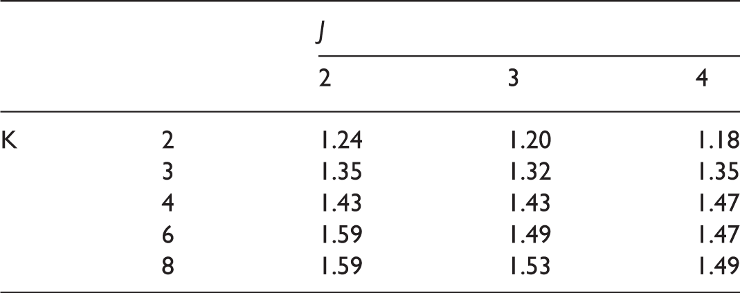
Although efficiency (in terms of maximum sample size) can be gained by deviating from an equal allocation to each arm, the gain is generally fairly small (as also shown by Wassmer²⁷). Figure 1(a) shows the maximum sample size for the three-stage triangular design with the TAILoR design parameters across a range of allocation ratios. By choosing the optimal allocation ratio, the maximum sample size is reduced by only 2.5% compared to an equal allocation. Interestingly, one has to increase the allocation to controls considerably in order to noticeably increase the maximum sample size. Put conversely this implies that a large number of patients can be put on the control treatment without inflating the maximum sample size considerably. This may, for example, be of interest if the control treatment is considerably cheaper than the experimental treatments or thought to have a better safety profile than the experimental treatments. This effect is shown in Figure 1(b), where the total cost of allocating patients is shown as the ratio of the cost of the control treatment and experimental treatments varies. If the cost of the control treatment is very low, then a high allocation to control patients would be optimal.

Figure 1.

Maximum sample size and maximum cost (arbitrary units) of treatment as allocation ratio changes. Designs are chosen using triangular stopping boundaries such that they give 5% type-I error and 90% power. Maximum cost assumes that the cost of allocating a patient to the control group is c, and the cost of allocating a patient to an experimental treatment is 1 where c ∈ {1, 0.5, 0.25, 0.1}.

The downside of allocating additional patients to the control treatment is that it may reduce recruitment to the trial. There is some evidence that in placebo controlled trials, patient willingness to take part in the trial is reduced as the allocation to the control group increases.²⁸

5 Unknown variance

For trials with a normally distributed endpoint, a common assumption made at the design stage is that the variance, σ², is known. Of course this is not generally the case, and even if a prior estimate of the variance is available, it is usually subject to considerable uncertainty. Using a test statistic that assumes a known variance will lead to incorrect operating characteristics if the actual variance differs from the quantity assumed in the test statistic. For group-sequential trials, several papers have suggested approaches to modifying stopping boundaries to allow for unknown variance including Monte Carlo simulation,²⁹ a recursive algorithm³⁰ and quantile substitution, i.e. replacing the stopping boundaries, which are quantiles of the standard normal distribution, with the equivalent quantiles of Student's t-distribution, as described in Jennison and Turnbull.³¹ Currently there is no work on extending the recursive algorithm to group-sequential MAMS trials; instead we examine the third method, which is straightforward and not computationally intensive.

Recall that l_j and u_j are the stopping boundaries for analysis j, and jn is the number of patients per arm that are randomised by the time of the analysis. Then the thresholds for stopping in terms of p-values are attained from the respective quantiles of the normal distribution, i.e. 1 − Φ(u_j) and 1 − Φ(l_j) respectively. With unknown variance, when δ = 0, the test-statistics would be marginally distributed as a Student's t-distribution with 2jn − 2 degrees of freedom. A natural approach to take the unknown variance into consideration is to find new stopping boundaries as $f' j = T_{2 jn - 2} (1 - Φ (l_{j}))$ and $e_{j}^{'} = T_{2 jn - 2} (1 - Φ (u_{j}))$ , where T_p is the cumulative distribution function of Student's t-distribution with p degrees of freedom.

To evaluate whether the quantile-substitution method works adequately for MAMS trials, we compare the FWER and power for three different approaches. The first is to use the known variance test statistic with presumed value of σ; the second is to use a t-test without modifying the stopping boundaries; and the third approach is to use the t-test together with using quantile substitution to change the stopping boundaries. The following two designs are considered:

n = 35, f = (0, 1.44, 2.34), e = (2.71, 2.39, 2.34) a three-stage four experimental arm triangular design when δ₀ = 0.178, δ₁ = 0.545, σ = 1, α = 0.05, 1 − β = 0.9;

n = 10, f = (0, 1.43, 2.34), e = (2.70, 2.39, 2.34) a three-stage four experimental arm triangular design for δ₀ = 0, δ₁ = 1, σ = 1, α = 0.05, 1 − β = 0.9.

Tables 3 and 4 show the estimated FWER and power from 100,000 independent replicates for each design as the true value of σ varies. Clearly assuming known variance leads to unacceptable type-I error inflation when the true value of σ is above the design value. For the design with the group size of 35, just using the known-variance stopping boundaries together with the t-test leads to a mild inflation in the FWER (on average, the FWER is around 0.054). However, the inflation is much greater when the group size is 10 (FWER of around 0.070). Modifying the stopping boundaries using quantile-substitution leads to correct nominal FWER for n = 35 and a very small inflation for n = 10.

Table 3.

FWER and power estimates as the true standard deviation varies from the assumed value of 1 for three-stage design with four experimental arms, n = 35, f = (0, 1.44, 2.34), e = (2.71, 2.39, 2.34). 100,000 independent replicates used to estimate type-I error and power. Z-test is using the original boundaries with a Z-statistic, t-test the original boundaries with a t-statistic while t-test^corr uses a t-statistic with corrected boundaries. Monte Carlo standard error for estimated type-I error ≈ 0.0007. Maximum Monte Carlo standard for power estimate ≈0.0015

	Type-I error			Power
σ	Z-test	t-test	t-test^corr	Z-test	t-test	t-test^corr
0.25	0.000	0.054	0.050	1.000	1.000	1.000
0.5	0.000	0.054	0.050	0.999	0.997	0.997
0.75	0.005	0.056	0.051	0.975	0.973	0.975
1	0.049	0.054	0.049	0.900	0.892	0.893
1.25	0.140	0.055	0.050	0.791	0.730	0.728
1.5	0.236	0.053	0.049	0.691	0.562	0.558
1.75	0.327	0.054	0.050	0.613	0.432	0.426
2	0.396	0.054	0.050	0.549	0.330	0.325

Table 4.

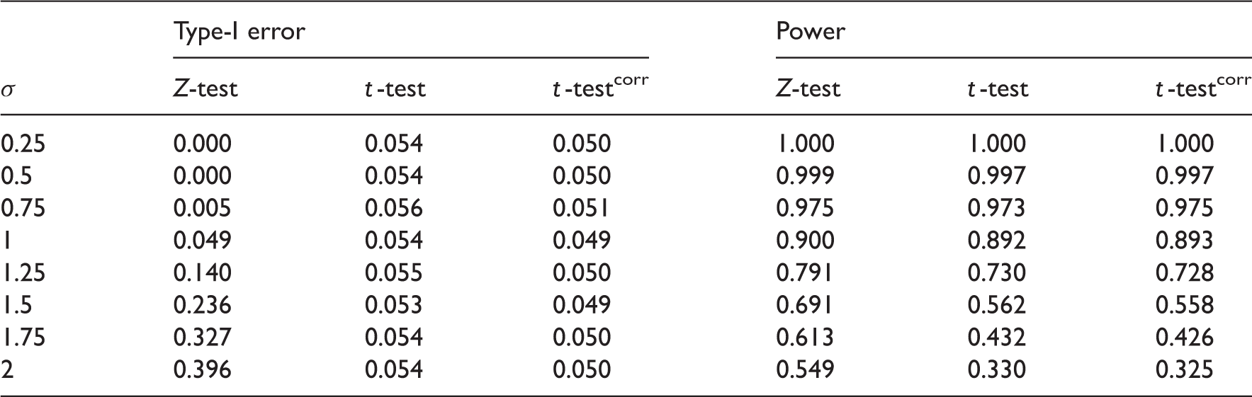
FWER and power estimates as the true standard deviation varies from the assumed value of 1 for three-stage design with four experimental treatments, n = 10, f = (0, 1.43, 2.34), e = (2.70, 2.39, 2.34). 100,000 independent replicates used to estimate type-I error and power. Z-test is using the original boundaries with a Z-statistic, t-test the original boundaries with a t-statistic while t-test^corr uses a t-statistic with corrected boundaries. Monte Carlo standard error for estimated type-I error ≈0.0007. Maximum Monte Carlo standard for power estimate ≈0.0015

	Type I error			Power
σ	Z-test	t-test	t-test^corr	Z-test	t-test	t-test^corr
0.25	0.000	0.069	0.053	1.000	1.000	1.000
0.5	0.000	0.069	0.052	0.999	1.000	1.000
0.75	0.005	0.069	0.052	0.976	0.993	0.993
1	0.051	0.070	0.052	0.910	0.918	0.911
1.25	0.140	0.068	0.051	0.853	0.758	0.740
1.5	0.238	0.070	0.053	0.777	0.587	0.562
1.75	0.326	0.069	0.052	0.707	0.455	0.429
2	0.398	0.069	0.052	0.642	0.355	0.328

Modifying the stopping boundaries is not sufficient to control both the FWER and power as σ varies from its design value. In confirmatory trials, the priority should be placed on controlling the FWER, which appears to be possible using quantile-substitution. If one wishes to simultaneously control the FWER and power, a sample-size reestimation technique could be applied as better estimates of σ are gathered throughout the trial. An alternative approach is to use a p-value combination test design,^8,9 in which case an exact solution for unknown variance is available.²⁷

6 Adding treatment arms

In some situations it may be of interest to add additional experimental arms to the study after the study has already been started. The MRC STAMPEDE trial,¹² for example, has recently added a further treatment arm due to excellent recruitment rates. If controlling the FWER is of interest, then adding new treatments is in general not advisable as the properties of the study in terms of FWER and power will be altered. Instead we aim to show the impact of adding treatments without adjusting the design and to provide simple adjustments that can be made to maintain FWER control under a specific situation. We consider a two-stage design with four experimental arms. Assuming equal numbers of patients in each arm in each stage, the resulting boundaries, l and u, and sample size per arm per stage, n, can be found in Table 5 for triangular, O'Brien–Flemming and Pocock boundaries where the latter two designs are constrained by setting l₁ = 0.

Table 5.

Error rates when treatment is added at interim, keeping the original boundaries. Based on 100,000 simulations

Design	l	u	n	${\overset{\land}{α}}_{+}$	$1 - {\overset{\land}{β}}_{+}$	$1 - {\overset{\land}{β}}_{+}^{*}$
OBF	(0,2.169)	(3.068,2.169)	44	0.059	0.903	0.870
P	(0,2.375)	(2.375,2.375)	50	0.056	0.903	0.739
T	(0.811,2.293)	(2.432,2.293)	50	0.057	0.901	0.767

We start by considering a, somewhat unrealistic, scenario in which one additional experimental treatment arm is always added at the interim. An additional 2n patients are recruited to treatment k = 5 in the second stage and an additional test statistic, $Z_{2}^{(5)}$ is calculated and compared to the boundaries at the end of the study. Table 5 provides Monte Carlo estimates of the FWER, ${\overset{\land}{α}}_{+}$ , and the power under the LFC, $1 - {\overset{\land}{β}}_{+}$ , when the original boundaries are used for making test decisions. As expected there is a clear inflation of the FWER over the nominal α = 0.05 while the effect on power is negligible in these examples.

Since the fifth treatment can never stop early, the power is no longer independent of the treatment labels so that it is of interest to also investigate the power to select treatment 5 under the LFC. The corresponding Monte Carlo estimate, $1 - {\overset{\land}{β}}_{+}^{*}$ , can be found in Table 5. From that it can be seen that the chance of recommending the newly added treatment is considerably lower than the anticipated power even if the treatment has a worthwhile effect.

It is, however, possible to control the type-I error rate if a fifth treatment is always added by finding values of l₁, u₁, u₂ (either numerically or via simulation) such that the probability of making a type-I error is controlled. The simulations given in Table 6 confirm the adjusted boundaries control the FWER – the power is, however, reduced.

Table 6.

Error rates when treatment is added at interim, adjusting the upper boundary at the second stage. Based on 100,000 simulations

Design	$u_{2}^{adj}$	${\overset{\land}{α}}_{+}$	$1 - {\overset{\land}{β}}_{+}$	$1 - {\overset{\land}{β}}_{+}^{*}$
OBF	2.245	0.051	0.893	0.862
P	2.455	0.051	0.894	0.730
T	2.384	0.051	0.892	0.755

A more realistic setting than the one described above is when a treatment is added only with probability p⁺. In this case the original boundaries are used when no treatment is added while adjusted boundaries are used otherwise.

Consider the design in Table 5 with the O'Brien–Flemming shaped upper boundary: l₁ = 0, u₁ = 3.068, u₂ = 2.169. Table 7 contains the adjusted second stage upper boundaries when it is pre-planned to add 1, 3 and 10 new treatments at the interim analysis. Now consider two mechanisms for adding the additional treatments. If the treatments are added (and the adjusted upper boundary is used) with probability p⁺ = 0.5, independent of the first stage data, the simulations presented in Table 7 confirm that the familywise error rate is controlled. If, however, the treatments are only added when first-stage results are disappointing, e.g. when

max_{k = 1, \dots, K} Z_{1}^{(k)} < 1

, then the final column of Table 7 shows that the familywise error rate is inflated. Consequently it is crucial for the decision to add new treatments to be independent of the results obtained at interim.

Table 7.

Monte Carlo estimates of familywise error rate (target α = α₊ = 0.05) when K_new new treatments are added independently or on the basis of disappointing first stage results. Based on original OBF design, l₁ = 0, u₁ = 3.068, n = 44 and 100,000 simulations

K _new	$u_{2}^{adj}$	ℙ(Y⁺ = 1) = 0.5	Y⁺ = 1 if $max Z_{1}^{(k)} < 1$
1	2.245	0.051	0.052
3	2.353	0.051	0.053
10	2.561	0.050	0.054

7 Discussion

MAMS trials have an important role to play in improving the efficiency of the drug development process when several experimental treatments are awaiting testing. Parmar et al.³² propose MAMS trials as a way of achieving more reliable results more quickly when evaluating new agents in cancer. A number of recent papers have discussed design of MAMS trials^{8,6,9,11,12,16,33} using a variety of different approaches.

In this article we have considered a multitude of issues in the design of MAMS trials. Our recommendations are as follows:

Strong control of the FWER should be considered a priority in the design of confirmatory MAMS trials.

A MAMS trial should be powered to recommend a clearly superior treatment, with the value of δ₁, the clinically relevant difference, being important; the value of δ₀ (i.e. the mean effect of the other treatments) is less important.

The efficiency benefits of a higher allocation of patients to control are low, and may be damaging to recruitment. However, if the control treatment is considerably cheaper than other treatments, then a higher allocation may lead to large cost reduction without compromising the design characteristics.

If the group size is low (below 20), stopping boundaries should be adjusted using quantile substitution to account for unknown variance when considering normally distributed endpoints.

For confirmatory MAMS trials, we do not recommend adding treatment arms on the basis of interim results. In the case of experimental treatment arms being added for other reasons, subsequent stopping boundaries should be adjusted to maintain the FWER at the level specified at the design stage.

Footnotes

Acknowledgements

The views expressed in this publication are those of the authors and not necessarily those of the NHS, the National Institute for Health Research or the Department of Health. We thank the two anonymous reviewers for their useful comments.

Declaration of conflicting interests

The author(s) declared no potential conflicts of interest with respect to the research, authorship, and/or publication of this article.

Funding

The author(s) disclosed receipt of the following financial support for the research, authorship, and/or publication of this article: This work was funded by the Medical Research Council (grant numbers G0800860 and MR/J004979/1). This report is independent research arising from Dr Jaki’s Career Development Fellowship (NIHR-CDF-2010-03-32) supported by the National Institute for Health Research.

References

Kola

Landis

. Can the pharmaceutical industry reduce attrition rates?. Nature Rev Drug Discov 2004; 3: 711–716.

DiMasi

Hansen

Grabowski

. The price of innovation: new estimates of drug development costs. J Health Econ 2003; 22: 151–185.

Stallard

Todd

. Sequential designs for phase III clinical trials incorporating treatment selection. Stat Med 2003; 22: 689–703.

Thall

Simon

Ellenberg

. Two-stage selection and testing designs for comparative clinical trials. Biometrika 1988; 75: 303–310.

Whitehead

Jaki

. One- and two-stage design proposals for a phase II trial comparing three active treatments with a control using an ordered categorical endpoint. Stat Med 2009; 28: 828–847.

Stallard

Friede

. A group-sequential design for clinical trials with treatment selection. Stat Med 2008; 27: 6209–6227.

Kelly

Stallard

Todd

. An adaptive group sequential design for phase II/III clinical trials that involve treatment selection. J Biopharmaceut Stat 2005; 15: 641–658.

Posch

Konig

Branson

. Testing and estimation in flexible group sequential designs with adaptive treatment selection. Stat Med 2005; 24: 3697–3714.

Bretz

Konig

Brannath

. Adaptive designs for confirmatory clinical trials. Stat Med 2009; 28: 1181–1217.

10.

Royston

Parmar

MKB

Qian

. Novel designs for multi-arm clinical trials with survival outcomes with an application in ovarian cancer. Stat Med 2003; 22: 2239–2256.

11.

Magirr

Jaki

Whitehead

. A generalized Dunnett test for multiarm-multistage clinical studies with treatment selection. Biometrika 2012; 99: 494–501.

12.

Sydes

Parmar

MKB

James

. Issues in applying multi-arm multi-stage methodology to a clinical trial in prostate cancer: the MRC STAMPEDE trial. Trials 2009; 10

13.

O'Brien

Flemming

. A multiple-testing procedure for clinical trials. Biometrics 1979; 35: 549–556.

14.

Committee for proprietary medicinal products. Points to consider on multiplicity issues in clinical trials. Technical report, EMEA, 2002.

15.

Dunnett

. A multiple comparison procedure for comparing several treatments with a control. Journal of the American Statistical Association 1955; 50: 1096–1121.

16.

Wason

JMS

Jaki

. Optimal design of multi-arm multi-stage trials. Stat Med 2012 (E-published.

17.

Freidlin

Korn

Gray

. Multi-arm clinical trials of new agents: some design considerations. Clin Cancer Res 2008; 14: 4368–4371.

18.

Dunnett

Santner

Tamhane

. Selection of the best treatment in comparison to a control with an application to a medical trial. Design of experiments: ranking and selection New York: Marcel Dekker, 1984, 47–66.

19.

Whitehead

Stratton

. Group sequential clinical trials with triangular continuation regions. Biometrics 1983; 39: 227–236.

20.

Pocock

. Group sequential methods in the design and analysis of clinical trials. Biometrika 1977; 64: 191–199.

21.

Lan

KKG

DeMets

. Discrete sequential boundaries for clinical trials. Biometrika 1983; 70: 659–663.

22.

Wason

JMS

Mander

. Minimising the maximum expected sample size in two-stage phase II clinical trials with continuous outcomes. J Biopharmaceut Stat 2011 (in press.

23.

Wason

JMS

Mander

Thompson

. Optimal multi-stage designs for randomised clinical trials with continuous outcomes. Stat Med 2012; 31: 301–312.

24.

Wang

Tsiatis

. Approximately optimal one-parameter boundaries for group sequential trials. Biometrics 1987; 43: 193–199.

25.

Pampallona

Tsiatis

. Group sequential designs for one-sided and two-sided hypothesis testing with provision for early stopping in favor of the null hypothesis. J Stat Plan Infer 1994; 42: 19–35.

26.

Wason

JMS

. OptGS: An R package for finding near-optimal group-sequential designs. J Stat Softw 2013 (Accepted.

27.

Wassmer

. On sample size determination in multi-armed confirmatory adaptive designs. J Biopharmaceut Stat 2011; 21: 802–817.

28.

Halpern

Karlawish

JHT

Casarett

. Hypertensive patients' willingness to participate in placebo-controlled trials: implication for recruitment efficiency. Am Heart J 2003; 146: 985–992.

29.

Shao

Feng

. Group sequential t-tests for clinical trials with small sample sizes across stages. Contemp Clin Trials 2007; 28: 563–571.

30.

Jennison

Turnbull

. Exact calculations for sequential t,χ²and f tests. Biometrika 1991; 78: 133–141.

31.

Jennison

Turnbull

Group sequential methods with applications to clinical trials 2000, Boca Raton: Chapman and Hall.

32.

Parmar

MKB

Barthel

FM-S

Sydes

. Speeding up the evaluation of new agents in cancer. J Nat Cancer Inst 2008; 100: 1204–1214.

33.

Friede

Parsons

Stallard

. Designing a seamless phase II/III clinical trial using early outcomes for treatment selection: an application in multiple sclerosis. Stat Med 2011; 30: 1528–1540.