A Dynamic Relationship between Financial Development and Import Demand for Bangladesh: An Evidence from Combine Cointegration and Granger Causality Approach

Abstract

This article has estimated the impact of financial development on import demand over the period of 1986: Q1–2014: Q4 in case of Bangladesh. The long-run relationship between financial development, import demand and economic growth are investigated by combine cointegration. Error Correction Method (ECM) is applied to examine short-run phenomena. The unit root properties of variables are tested by augmented Dickey–Fuller test (ADF) and Philips–Perron (P–P) unit root test. Perron (1997) single structural break unit root test is also applied. The results of Bayer and Hanck (2013) combine cointegration test that reveal the existence of long-run relationship between import demand, financial development and economic growth. Financial development and economic growth have a positive and significant impact on import demand in long run as well as in short run. The lagged value of error correction method (ECMt-1) is –0.08 that is negative and significant. This indicates that change from equilibrium level of import demand is corrected by 8 per cent per quarter in a year. The results of Vector Error Correction Model (VECM) Granger causality explain that bidirectional causality exists between import demand and financial development in long run as well as short run. Similarly, bidirectional causality exists between import demand and economic growth in short run. Policymakers should focus on financial sector development for import of technology through adoption of the import substitution policy.

Keywords

Financial development import demand combine cointegration VECM Granger causality Bangladesh

Introduction

Trade liberalization has become an essential part of every economy. Due to trade liberalization, both physical and human capital are moving across the borders (Jaimovich & Kamuganga, 2010). Additionally, free market information, building trade zones and continuous trade agreements have developed the production process around the world. The impact of trade liberalization on imports is indirectly linked to price changes that effect consumption decisions. In developing economies, the unavailability of sufficient funds leads to a reduction in domestic demand along with an inflationary pressure in the domestic market. Therefore, especially for developing economies, a sustainable import demand function is needed until the development of domestic production does not increase. There are two schools of thought for import restrictions, Trade Pessimists and Trade Optimists. Trade Pessimists are in favour of import restriction via import tariff and quota, whereas Trade Optimists are in favour of free trade.

The classical trade demand theory was linked with consumer’s objective of utility maximization. This objective was primarily linked to income level and/or price level. Similarly, the aggregate demand for all individuals constitute a national demand for imports (Harrod & Hague, 1963, p. 464). The imports take place because of excess domestic demand as compared to domestic supply. Therefore, income elasticity of imports can be negative if domestic demand is inelastic. Moreover, import prices are also a pivotal determinant of demand for imports. An increase in price of import changes purchasing capacity and supply of imports (Caves & Jones, 1985). Similarly, the exchange rate volatility has a negative effect on trade. When a change in exchange rate accrues uncertainly, the confidence of investor declines that leads to decrease in trade. The theoretical literature explains that exchange rate volatility has less effect on trade volume in developing countries. Relatively, it focuses upon the income level of the consumer as more important factor for changes in import demand as compared to price effect (De-Grauwe, 1988).

The financial sector development of any economy helps to support import demand function. More financial support benefits to overcome the balance of payment problem. A developed financial sector also helps to import finish or final goods and services in the domestic market. Import of technological equipment and knowledge push upward new innovations at home that enhance economic growth by upgrading the existing level of production. The financial development changes the spectrum of production in developing economies. Bangladesh adopted trade liberalization policy for the concern of international trade in 1985. Following the Structural Adjustment Programmes (SAP) initiated by the International Monetary Fund (IMF), the restricted items were minimized to 4 in 2006 which were 478 in 1986. Similarly, the custom duty rate was dropped from 350 per cent in 1992 to 25 per cent in 2006. The average import weighted tariff on final consumer goods was 47.3 per cent in 1992 that reduced to 13.4 per cent in 2006. On intermediate inputs, the average import weighted tariff was 24.1 per cent in 1991 that reduced to 9.33 per cent in 2006 (Bangladesh Bureau of Statistics (BBS) and National Board of Revenue (NBR), Bangladesh).

Bangladesh also supported the IMF obligations of Article 8 and subsidies were taken out from many items of import and export. International trade played a pivotal role in import of merchandise, export of intermediate inputs and technology transfer that increased economic growth through enhancing domestic exports (Hoque & Yusop, 2010). All imports as a percentage of gross domestic product (GDP) were 11.3 per cent in 1973 that increased to 21.82 per cent in 2006. Similarly, the import of consumer goods as a percentage of GDP were 20.58 per cent in 1981 which decreased to 9.25 per cent in 2005. For capital items, the imports were 17.19 per cent in 1981 but decreased to 1.67 per cent in 2005. Meanwhile, the nominal GDP in local currency was 67,813 in 1973 but increased to 3,707,370 in 2006 (BBS and NBR).

The contribution of this study in applied economics is to check the impact of financial development on import demand for Bangladesh over the period of 1986: Q₁–2014: Q₄. The long-run relationship between variables is predicted by applying the new cointegration approach called ‘Bayer–Hanck combine cointegration’. The direction of causality is examined by applying Vector Error Correction Model (VECM) Granger causality approach. The rest of the article is organized as follows: review of literature is described in the second section. The third section explains data collection, model development and estimation technique. Empirical estimations and their results are described in the fourth section. The fifth section is for conclusion and recommendations.

Literature Review

Existing literature focuses on the direct relationship between financial development and economic growth of developing economies (Ahmed & Ansari, 1988; Altunç, 2008; Aslan & Korap, 2007; Fase & Abma, 2003; Robinson, 1952; Shahbaz & Lean, 2012). While financial development led import demand function can be regarded as an indirect way to economic growth, Burgess (1974) explained imports by classical trade theories and argued that mostly finished goods have substitutes in the home market. The demand for imports of finished goods is dependent upon the factor endowed in an economy. Therefore, empirical evidence of demand for imports holds significance in modern literature.

Mah (2000) empirically evaluated the import demand of information technology products over the period of 1980–1997 in Korea. Auto Regressive Distributed Lagged (ARDL) approach predicted that cointegration exist between import duty, import price index, producer price index and real GDP. Similarly, Dutta and Ahmed (2004) probed the import demand function of India for the time span of 1971–1995. The results of Johansen cointegration approach showed a long-run cointegration between real quantity of import merchandise, real GDP and relative import price. The VECM indicated that Indian import demand function is more related to the growth of real GDP as compared to relative import prices. S. Narayan and P. K. Narayan (2005) investigated disaggregate import demand function by using an ARDL approach for Fiji. They used relative prices, investment expenditures, export expenditure and total consumption. Their results displayed a long-run cointegration among variables. It also showed that investment expenditure, total consumption and export expenditure have a positive, inelastic and significant impact on import demand of Fijian economy.

Chen (2008) used ARDL approach to estimate the import demand function of Taiwan by using the time period 1976Q₁ to 2004Q₁. The results revealed a long-run relationship between price ratio, real GDP and aggregate imports. Moreover, income elasticity was elastic in both long run and short run. Further, Ziramba (2010) analysed the import demand of crude oil for South African economy over the period of 1980–2006. The results of Johansen cointegration approach exposed a long-run relationship between quantity of imported crude oil, real price of crude oil and real GDP. The results also showed a negative relationship of real GDP, but a positive relationship of real crude oil price with quantity of imported crude oil. Similarly, the short-run results showed positive but insignificant impact of explanatory variables on quantity of crude oil import by South African economy. Yue (2010) targeted disaggregated import demand function of Cote d’Ivoire for the time span of 1970–2007. Using ARDL approach, the results confirmed a cointegration relationship between import demand, final consumption expenditure, investment expenditure, relative prices and export expenditure. The results revealed that exports and investment expenditures are the most potential determinants of import demand in long run.

Yin and Hamori (2011) analysed import demand function for Chinese economy over the period of 1978–2009. They used an ARDL approach to check cointegration between volume of import, real income, relative price, final consumption expenditure, real public consumption expenditures, real private consumption expenditures, real investment expenditures and real export expenditures. The results displayed that cointegration exist between selected variables. Moreover, real public expenditure has a negative relationship with import demand of China. Similarly, Wang and Lee (2012) reinvestigated import demand function of Chinese economy using monthly data from 1992m₁–2011m₁₂. The results showed that a long-run relationship exist between import volume, domestic income, real effective exchange rate and volatility of US market. Their results revealed that domestic income has a positive and significant impact on import volume while real effective exchange rate has a negative impact on import volume. Alam (2012) investigated import demand function for Pakistan over the time span 1979Q₁–2005Q₄. The results of ARDL approach confirmed the presence of cointegration between real imports, real effective exchange rate, real income and exchange rate volatility. It also concluded that merchandise import demand is income inelastic. Moreover, real effective exchange rate has a negative impact on import demand for Pakistan.

There are very few studies that investigated the import demand function for Bangladesh such as Kabir (1988) has used price index of domestic substitutes, price index of imports and income to evaluate the import demand function for Bangladesh for a time span of 1973Q₁–1983Q₄. Cochrane–Orcutt (CORC) estimation procedure has followed to investigate the import demand function of Bangladesh. The results showed that income and relative price have a positive and negative relationship with import demand, respectively. Dutta and Ahmed (1999) examined import demand function for Bangladesh over the period of 1974–1994. Engle–Granger and Johansen cointegration approaches have been used to analyse the relationship between real quantities of imports, real foreign exchange reserves, real import prices and real GDP. Their results revealed the existence of cointegration vector between variables. Moreover, Hassan and Islam (2005) estimated the import demand function for Bangladesh over the period of 1974Q₁–1998Q₄. The Johansen–Juselius cointegration approach indicated the long-run relationship between import price, income, industrial production and domestic prices.

Hye and Siddiqui (2010) probed an import demand function for Bangladesh over the period of 1980–2008. ARDL model has been used to analyse the long-run relationship between variables. Their results showed the existence of cointegration between import prices, domestic price and gross national product (income). The results also exposed that income has a positive impact on import demand, but relative prices have a negative impact on import demand of Bangladesh. Similarly, Hoque and Yusop (2010) analysed the impact of trade liberalization on import demand function of Bangladesh using ARDL approach for the time span of 1973–2005. Their results confirm a long-run relationship between real quantity of merchandise imports, relative prices of imports, real income, real foreign exchange reserves and dummy variables for import liberalization. Further, Aziz (2013) used both Engle–Granger and Johansen cointegration approach to find the import demand function over the period of 1978–2008 for Bangladesh. The results predicted a long-run cointegration between volume of imports, relative prices, real income and foreign exchange reserves. Moreover, relative prices have a negative relationship with import demand while income and foreign exchange have a positive relationship with import demand of Bangladesh.

By analysing existing literature, we predict that there are many factors that are affecting import demand such as income, imports prices, domestic prices, relative prices expenditures, national cash flow, investment, exports, domestic prices, and foreign remittances. Existing literature has ignored the role of financial development in investigating import demand function for Bangladesh. This study extends the previous literature by adding financial development as a potential determinant of import demand for Bangladesh. Financial development plays a significant part in explaining import demand. Financial sectors provide finance to firms for investment purposes that increase capitalization. Further, it helps to import inputs and technologies to enhance domestic production. Similarly, Beck (2002) argued that more availability of finance helps domestic merchandise importers to produce goods at home with cheaper rates.

Data Collection, Model Construction and Methodology

The aim of this study is to investigate the relationship between financial development, import demand and economic growth by using quarterly time series data from 1986: Q₁–2014: Q₄ for Bangladesh. For this purpose, we use log-linear specification because log-linear specification has superior properties to simple linear specification. The former provides efficient and consistent empirical findings as compared to the latter one. The functional form and log-linear form of models are as follows:

I_{t} = f (F d_{t}, Y_{t})

(1)

\ln I_{t} = β_{0} + β_{1} \ln F d_{t} + β_{2} \ln Y_{t} + μ_{t}

(2)

Here ln I_t is natural log of import of goods and services proxy for import demand, ln Fd_t is natural log of domestic credit to private sector as a percentage of GDP proxy for financial development, ln Y_t is natural log of real GDP per capita proxy for economic growth and µ_t is error term. The data of all series are collected from world development indicator (WDI) and international financial statistics (IFS). We have used quadratic match-sum method to transform annual data series into quarter frequency data.

Standard cointegration approaches are concerned with level of integration. For this purpose, we have applied Philips–Perron (P–P) unit root test to check whether series are integrated at level I(0) or 1st difference I(1). There are several techniques in time series literature to address the issue of cointegration such as Engle and Granger (1987) cointegration approach, Johansen (1991) Johansen maximum Eigen value test, Phillips and Ouliaris (1990) Phillips-Ouliaris cointegration test and Error Correction Method (ECM) based F-test of Peter Boswijk (1994), and the ECM based t-test of Banerjee, Dolado and Mestre (1998). All these approaches provide different results due to some deficiencies.

Bayer and Hanck Combine Cointegration

Bayer and Hanck (2013) invented combine cointegration based on several cointegration techniques to enhance the power of cointegration. Bayer and Hanck (2013) called this approach as combine cointegration. The null hypothesis states that there is no cointegration between series. Following Bayer and Hanck (2013), the combination of the computed significance level (p-value) of individual cointegration test in this article is given in Fisher’s formulas as follows:

E G - J O H = - 2 [\ln (P_{E G}) + (P_{J O H})]

(3)

E G - J O H - B O - B D M = - 2 ​ [\ln (P_{E G}) + (P_{J O H}) + (P_{B O}) + (P_{B D M})]

(4)

where P_EG, P_JOH, P_BO and P_BDM are the p-values of various individual cointegration tests, respectively. It is assumed that if the estimated Fisher statistics exceed the critical values provided by Bayer and Hanck (2013), the null hypothesis of no cointegration is rejected.

VECM Granger Causality Approach

When cointegration exist between variables, we move towards VECM Granger causality to test the direction of causality. The Granger causality test with VECM framework is as follows:

Δ L I_{t} = ϑ_{1} + \sum_{i = 1}^{p} ϑ {}_{i}Δ L I {}_{t = i}+ \sum_{j = 1}^{q} ϑ {}_{j}Δ L F d {}_{t = j}+ \sum_{k = 1}^{n} ϑ {}_{k}Δ L Y {}_{t = k}+ η_{1} E C M_{t - 1} + μ_{i}

(5)

Δ L F d_{t} = λ_{1} + \sum_{i = 1}^{p} λ {}_{i}Δ L F d {}_{t = i}+ \sum_{j = 1}^{q} λ {}_{j}Δ L I {}_{t = j}+ \sum_{k = 1}^{n} λ {}_{k}Δ L Y {}_{t = k}+ η_{2} E C M_{t - 1} + μ_{i}

(6)

Δ L Y_{t} = δ_{1} + \sum_{i = 1}^{p} δ {}_{i}Δ L Y {}_{t = i}+ \sum_{j = 1}^{q} δ {}_{j}Δ L I {}_{t = j}+ \sum_{k = 1}^{n} δ {}_{k}Δ L F d {}_{t = k}+ η_{3} E C M_{t - 1} + μ_{i}

(7)

where Δ is a difference, ECM represents the error correction term which is derived from long-run cointegration. ^₁, λ₁, δ₁ are constant and η (i = 1, 2, 3) are uncorrelated error term with zero mean. The optimal lag p is determined by Akaike Information Criterion (AIC) because of its superior properties for small data sets. The long-run causality is expressed by the significance of lagged ECM terms using t-test. For short-run causality is determined by F-statistics or Wald test.

Empirical Estimation and Results Interpretation

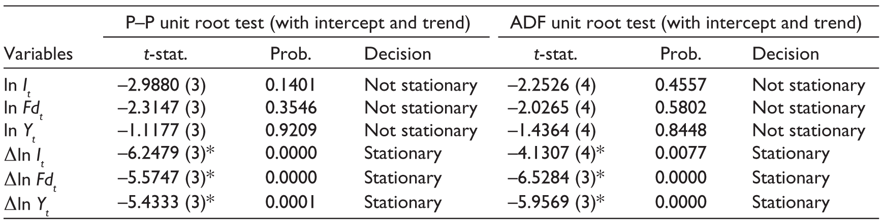
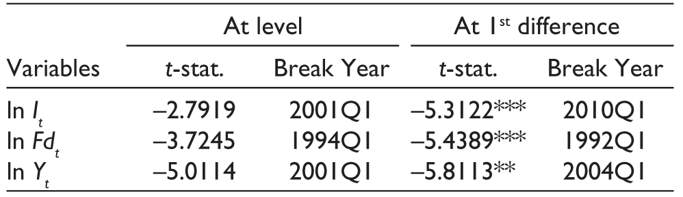
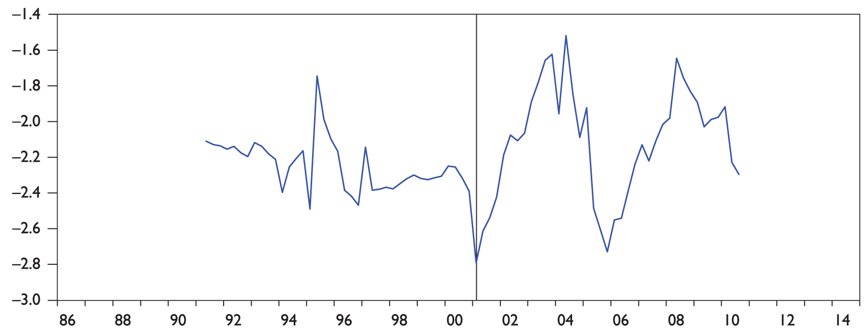
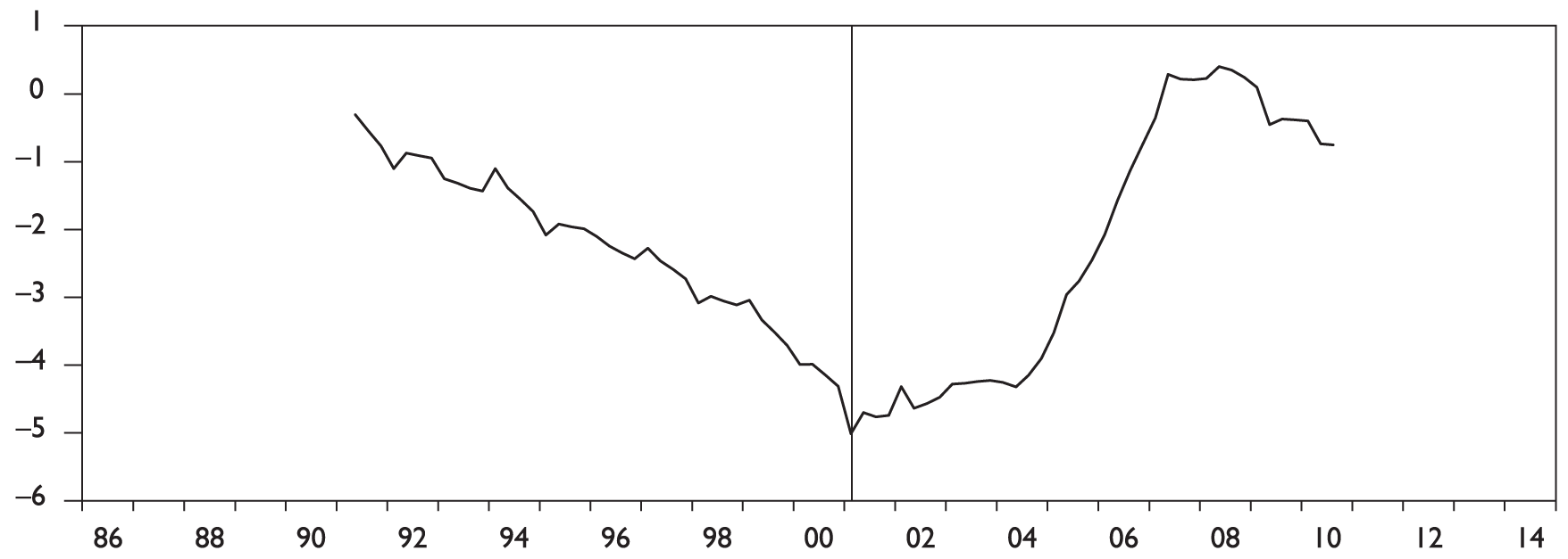
There are many traditional unit root tests such as augmented Dickey–Fuller test (ADF) by Dickey and Fuller (1981), P–P by Phillips and Perron (1988), DF–GLS by Elliot, Thomas and Stock (1996) and NG–Perron (2001) that help to test the unit root properties of data set. This study has applied ADF and P–P unit root tests to test the stationarity of data. The results of unit root tests are reported in Table 1. The results of ADF predict that all series have unit root problem at level I(0) but found to be stationary after taking 1st difference I(1). The robustness of ADF unit root test is tested by applying P–P unit root test. The results of P–P unit root test confirm the results of ADF unit root test, series are stationary. It shows that the results of ADF unit root test are reliable and consistent. Further, we apply Perron (1997) single structural break unit root test and the results are pasted into Table 2. The empirical evidence explains that import demand, financial development and economic growth have unit root problem at level with structural breaks. But, unit root problem does not seem when we take 1st difference. So, we may write that our series are integrated at 1st difference, that is, I(1). The structural break years such as 2001Q1, 1994Q1 and 2001Q1 belong to import demand, financial development and economic growth, respectively. These breaks can also be explained by Figure 1 for import demand, Figure 2 for financial development and Figure 3 for economic growth. Before we proceed to cointegration analysis, we find optimal lags through optimal lag selection criteria. Table 3 shows the results of optimal lag selection criteria. We follow the AIC for optimal lags due to its superior properties. The results indicate that 6 lags are suitable for our sample period. The results of other criterias such as sequential modified LR test statistic, Final prediction error, Schwarz information criterion and Hannan–Quinn information criterion are also reported in this table.

Table 1.

Unit Root Analysis

Variables	P–P unit root test (with intercept and trend)			ADF unit root test (with intercept and trend)
Variables	t-stat.	Prob.	Decision	t-stat.	Prob.	Decision
ln I_t	–2.9880 (3)	0.1401	Not stationary	–2.2526 (4)	0.4557	Not stationary
ln Fd_t	–2.3147 (3)	0.3546	Not stationary	–2.0265 (4)	0.5802	Not stationary
ln Y_t	–1.1177 (3)	0.9209	Not stationary	–1.4364 (4)	0.8448	Not stationary
Δln I_t	–6.2479 (3)*	0.0000	Stationary	–4.1307 (4)*	0.0077	Stationary
Δln Fd_t	–5.5747 (3)*	0.0000	Stationary	–6.5284 (3)*	0.0000	Stationary
Δln Y_t	–5.4333 (3)*	0.0001	Stationary	–5.9569 (3)*	0.0000	Stationary

Source: Authors’ calculations.

Notes: Significance at 1% is shown by * and lag values are shown in parentheses.

Table 2.

Perron (1997) Structural Break Unit Root

Variables	At level		At 1^st difference
Variables	t-stat.	Break Year	t-stat.	Break Year
ln I_t	–2.7919	2001Q1	–5.3122***	2010Q1
ln Fd_t	–3.7245	1994Q1	–5.4389***	1992Q1
ln Y_t	–5.0114	2001Q1	–5.8113**	2004Q1

Source: Authors’ calculations.

Note: ** and *** identify the significant at 5% and 10% level of significance, respectively.

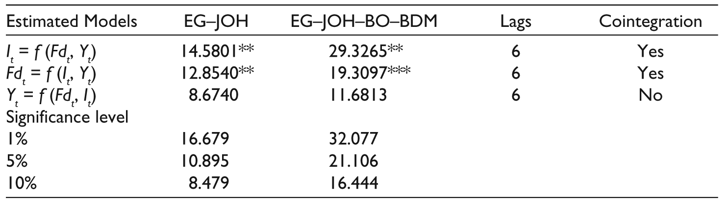
Our data series are integrated at a unique level that leads us to apply Bayer and Hanck’s (2013) combined cointegration to test the cointegration among variables. The results of combined cointegration are described in Table 4. The results explain that calculated F-statistics of EG–JOH and EG–JOH–BO–BDM for I_t = f (Fd_t, Y_t) are greater than critical values at 5 per cent level of significance. Similarly, the F-statistics of EG–JOH and EG–JOH–BO–BDM for Fd_t = f (I_t, Y_t) are larger than critical values at 5 per cent and 10 per cent level of significance, respectively. So we may reject the null hypothesis of no cointegration. These statistics confirm the existence of long-run relationship between financial development, import demand and economic growth. The existence of cointegration relationship explain co-movement between underlying variables. Once, we check the cointegration, it helps to predict movements between variables.

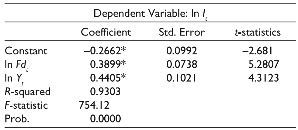
Table 5 displays the long-run estimations of import demand. The results reveal that financial development and economic growth have a positive and significant impact on import demand at 1 per cent significance level for Bangladesh. The coefficient of financial development is 0.38 which explains that 1 per cent increase in financial development leads to increase in import demand by 0.38 per cent. Similarly, a 1 per cent increase in economic growth leads to increase in import demand by 0.44 per cent. These results justify that the access of finance through financial sector development helps to import more goods that cause to increase in import demand. R-squared explains the portion of dependent variable that is explained by independent variables. So the results of R-squared explains that 93 per cent of import demand is explained by independent variables in long run. F-statistics shows significance of overall model. The value of F-statistics is significant at 1 per cent level of significance.

Figure 1.

Source: Authors’ estimation.

Figure 2.

Source: Authors’ estimation.

Figure 3.

Source: Authors’ estimation.

Similarly, the results of short-run analysis are explained by Table 6. According to results, financial development and economic growth also have a positive and significant impact on financial development at 1 per cent level of significance in short run. The coefficients of financial development and economic growth are 0.49 and 2.47 which explain that 1 per cent increase in financial development and economic growth will rise in import demand by 0.49 per cent and 2.47 per cent, respectively. So, we can also control import demand by controlling financial demand and economic growth. The lagged value of ECM is –0.0839 that is negative as expected and significant at 5 per cent level of significance. The value of ECM_(t–1) shows deviation from disequilibrium to equilibrium. This denotes that movement from short run towards long run are corrected by 8 per cent in each quarter and will take almost 12 years and 5 months to reach equilibrium path, if we use this model. The value of R-squared is 0.19 which shows that 19 per cent of import demand is explained by financial development and economic growth in short run. The overall model is good or/and fit due to significant of F-statistics at 1 per cent level of significance.

Table 3.

Lag-length Criteria

VAR Lag Order Selection Criteria
Lag	LogL	LR	FPE	AIC	SC	HQ
0	679.3512	NA	7.30e–10	–12.52502	–12.45052	–12.49481
1	1,447.070	1,478.569	5.77e–16	–26.57536	–26.27735	–26.45453
2	1,517.792	132.2772	1.84e–16	–27.71837	–27.19684	–27.50691
3	1,523.089	9.612761	1.97e–16	–27.64979	–26.90476	–27.34771
4	1,524.490	2.464496	2.28e–16	–27.50907	–26.54052	–27.11636
5	1,564.930	68.89784	1.28e–16	–28.09129	–26.89923	–27.60795
6	1,613.220	79.59004*	6.19e–17*	–28.81889*	–27.40333*	–28.24493*
7	1,616.630	5.430718	6.91e–17	–28.71538	–27.07630	–28.05079
8	1,617.668	1.595413	8.07e–17	–28.56793	–26.70534	–27.81272

Source: Authors’ calculations.

Notes: * indicates lag order selected by the criterion

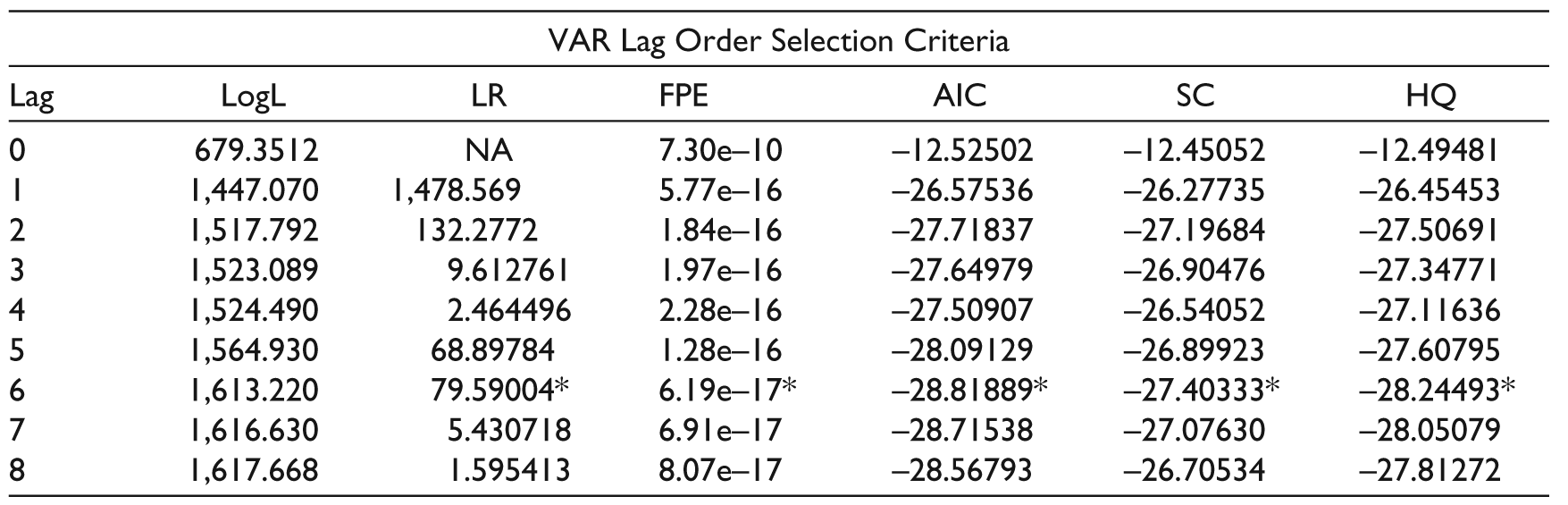
LR: sequential modified LR test statistic (each test at 5% level)

FPE: Final prediction error

AIC: Akaike information criterion

SC: Schwarz information criterion

HQ: Hannan–Quinn information criterion

Table 4.

Bayer and Hanck Combine Cointegration

Estimated Models	EG–JOH	EG–JOH–BO–BDM	Lags	Cointegration
I_t=f (Fd_t, Y_t)	14.5801**	29.3265**	6	Yes
Fd_t=f (I_t, Y_t)	12.8540**	19.3097***	6	Yes
Y_t=f (Fd_t, I_t)	8.6740	11.6813	6	No
Significance level
1%	16.679	32.077
5%	10.895	21.106
10%	8.479	16.444

Source: Authors’ calculations.

Notes: ** and *** represent significant at 5% and 10% level of significance. Lag length is based on minimum value of AIC.

Table 5.

Long-run Analysis

Dependent Variable: ln I_t
	Coefficient	Std. Error	t-statistics
Constant	–0.2662*	0.0992	–2.681
ln Fd_t	0.3899*	0.0738	5.2807
ln Y_t	0.4405*	0.1021	4.3123
R-squared	0.9303
F-statistic	754.12
Prob.	0.0000

Source: Authors’ calculations.

Note: Significance at 1% is shown by *.

Table 6.

Short-run Analysis

Dependent Variable: Δln I_t
	Coefficient	Std. Error	t-statistics
Constant	–0.0045*	0.0015	–2.9178
Δln Fd_t	0.4955*	0.1414	3.5030
Δln Y_t	2.4720*	0.6638	3.7235
ECM_t _–1	–0.0839**	0.0380	–2.2069
R-squared	0.1967
F-statistics	9.0637
Prob.	0.0000

Source: Authors’ calculations.

Note: Significance at 1% and 5% is shown by * and **, respectively.

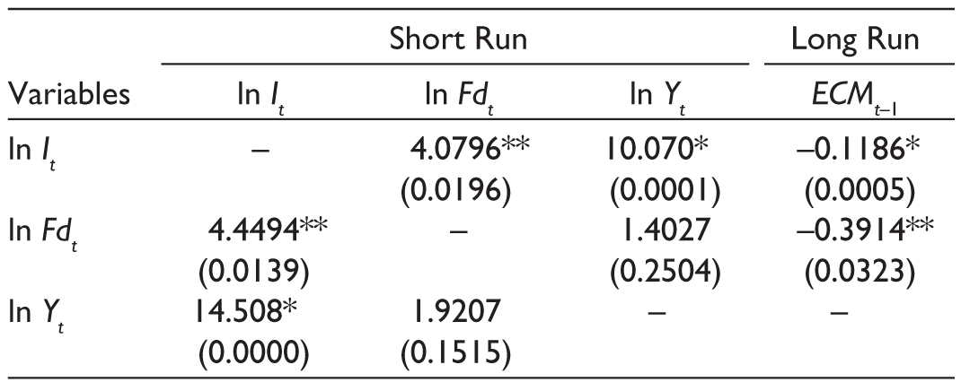
Once the cointegration has been confirmed between financial development, import demand and economic growth, we may proceed to detect the direction of causality to understand the clear picture of causal relationship. The Granger causality approach can be explained by the fact that X causes Y when the past value of X helps to predict changes of Y. Similarly, Y causes X when the changes of Y is predicted by the past value of X. Engle and Granger (1987) illustrated that if variables are cointegrating, there will be short-run and long-run information between them regarding to causal relationship. The vector autoregressive (VAR) model is likely to be used for this purpose. Table 7 describes the results of VECM Granger causality approach. The results reveal that bidirectional causality exists between financial development and import demand in short run as well as in long run. Economic growth causes import demand in both short and long run. Similarly, a unidirectional causality is running form import demand to economic growth only in short run. These findings are consistent with the findings of Shahbaz and Rahman (2012).

Table 7.

VECM Granger Causality Analysis

Variables	Short Run			Long Run
Variables	ln I_t	ln Fd_t	ln Y_t	ECM_t _–1
ln I_t	–	4.0796**(0.0196)	10.070*(0.0001)	–0.1186*(0.0005)
ln Fd_t	4.4494**(0.0139)	–	1.4027(0.2504)	–0.3914**(0.0323)
ln Y_t	14.508*(0.0000)	1.9207(0.1515)	–	–

Source: Authors’ calculations.

Note: Significance at 1%, 5% and 10% is shown by *, ** and ***, respectively.

Conclusion and Recommendations

The present study investigates the relationship between import demand, financial development and economic growth over the period of 1986: Q₁–2014: Q₄ for Bangladesh. The stationarity of data is tested by ADF and P–P unit root tests. After confirming the stationarity of data at 1st difference I(1), we have applied Bayer and Hanck’s combine cointegration approach to examine the long-run relationship between financial development, import demand and economic growth. The results have confirmed the presence of cointegration between variables for these models [I_t = f (Fd_t, Y_t) and Fd_t = f (I_t, Y_t)].

Further, financial development and economic growth both have positive and significant impact on import demand at 1 per cent level of significance. The lagged value of ECM explains the speed of adjustment from short run to long run. It will take approximately 12 years and 5 months to reach an equilibrium level. The results of VECM Granger causality explain the direction of causality. It has predicted that unidirectional causality exists between financial development import demand for both short and long run. Import demand and economic growth cause financial development only in long run but only import demand causes financial development in short run.

Policymakers should focus on financial development to control imports by adopting import substitution policy only for importing advance technology. An increase in financial reforms will help to develop new businesses through importing new technologies and machinery only. It will enhance domestic production and reduce dependence on import. It will help to reduce imports that further will increase the foreign reserves for Bangladesh. Financial sector development can be used as a tool control import demand.

Footnotes

Acknowledgements

The authors are thankful to the anonymous referees of this journal for their extremely useful comments and suggestions to improve the quality of this article. The usual disclaimers apply.

References

Ahmed

S.M.

& Ansari

M.I.

(1998). Financial sector development and economic growth: The South-Asian experience. Journal of Asian Economics, 9(3), 503–517.

Alam

(2012). A reassessment of Pakistan’s aggregate import demand function: An application of ARDL approach. The Journal of Developing Areas, 46(1), 367–384.

Altunç

Ö.F.

(2008). Türkiye’de Finansal Gelişme ve İktisadi Büyüme Arasındaki Nedenselliğin Ampirik Bir Analizi. Eskişehir Osmangazi Üniversitesi İİBF Dergisi, 3(2), 113–127.

Aslan

& Korap

H.L.

(2007). Monetary transmission mechanism in an open economy framework: The case of Turkey. Istanbul University Econometrics and Statistics E-Journal, 5(1), 41–66.

Aziz

(2013). Modelling import demand function for a developing country: An empirical approach. Asian–African Journal of Economics and Econometrics, 13(1), 1–15.

Banerjee

Dolado

& Mestre

(1998). Error-correction mechanism tests for cointegration in a single-equation framework. Journal of Time Series Analysis, 19(3), 267–283.

Bayer

& Hanck

(2013). Combining non-cointegration tests. Journal of Time Series Analysis, 34(1), 83–95.

Beck

(2002). Financial development and international trade: Is there a link? Journal of International Economics, 57(1), 107–131.

Boswijk

P.H.

(1994). Testing for unstable root in conditional and structural error correction models. Journal of Econometrics, 63(1), 37–60.

10.

Burgess

J.A.

(1974). Direct foreign investment in Eastern Europe: Problems and prospects of Romania’s joint venture legislation. Law and Pol’y Int’l Bus., 6(4), 1059.

11.

Caves

R.E.

& Jones

R.W.

(1985). World Trade and payments: An introduction (4th edn). Boston, MA: Little, Brown & Company.

12.

Chen

S.W.

(2008). Long-run aggregate import demand function in Taiwan: An ARDL bounds testing approach. Applied Economics Letters, 15(9), 731–735.

13.

De-Grauwe

(1988). Exchange rate variability and the slowdown in growth of international trade. Staff Papers–International Monetary Fund, 35(1), 63–84.

14.

Dickey

D.A.

& Fuller

W.A.

(1981). Likelihood ratio statistics for autoregressive time series with a unit root. Econometrica: Journal of the Econometric Society, 49(4), 1057–1079.

15.

Dutta

& Ahmed

(1999). An aggregate import demand function for Bangladesh: A cointegration approach. Applied Economics, 31(4), 465–472.

16.

Dutta

& Ahmed

(2004). An aggregate import demand function for India: A cointegration analysis. Applied Economics Letters, 11(10), 607–613.

17.

Elliot

G.R.

Thomas

& Stock

J.H.

(1996). Efficient tests for an autoregressive unit root. Econometrica: Journal of the Econometric Society, 64(4), 813–836.

18.

Engle

R.F.

& Granger

C.W.

(1987). Co-integration and error correction: Representation, estimation and testing. Econometrica: Journal of the Econometric Society, 55(2), 251–276.

19.

Fase

M.M.

& Abma

R.C.N.

(2003). Financial environment and economic growth in selected Asian countries. Journal of Asian Economics, 14(1), 11–21.

20.

Harrod

& Hague

D.C.

(Eds). (1963). International trade theory in a developing world. Springer: Macmillan.

21.

Hassan

A.K.

& Islam

M.R.

(2005). Temporal causality and dynamics of financial development, trade openness, and economic growth in vector auto regression (VAR) for Bangladesh, 1974–2003: Implication for poverty reduction. Journal of Nepalese Business Studies, 2(1), 1–12.

22.

Hoque

M.M.

& Yusop

(2010). Impacts of trade liberalisation on aggregate import in Bangladesh: An ARDL bounds test approach. Journal of Asian Economics, 21(1), 37–52.

23.

Hye

Q.M.A.

& Siddiqui

M.M.

(2010). Import demand function for Bangladesh: A rolling window analysis. African Journal of Business Management, 4(10), 2150–2156.

24.

Jaimovich

& Kamuganga

D.I.C.K.

(2010). Three decades of trade policy in Uganda: Two generations of reforms in the quest to become part of the global market. Frankfurt, Germany: Department of Applied Econometrics and International Economic Policy, Goethe University.

25.

Johansen

(1991). Estimation and hypothesis testing of cointegration vectors in Gaussian vector autoregressive model. Econometrica: Journal of the Econometric Society, 59(6), 1551–1580.

26.

Kabir

(1988). Estimating import and export demand function: The case of Bangladesh. The Bangladesh Development Studies, 16(4), 115–127.

27.

Mah

J.S.

(2000). An empirical examination of the disaggregated import demand of Korea: The case of information technology products. Journal of Asian Economics, 11(2), 237–244.

28.

Narayan

& Narayan

P.K.

(2005). An empirical analysis of Fiji’s import demand function. Journal of Economic Studies, 32(2), 158–168.

29.

& Perron

(2001). Lag length selection and the construction of unit root test with good size and power. Econometrica: Journal of the Econometric Society, 69(6), 1519–1554.

30.

Perron

(1997). Further evidence on breaking trend functions in macroeconomic variables. Journal of Econometrics, 80(2), 355–385.

31.

Phillips

P.C.B.

& Ouliaris

(1990). Asymptotic properties of residual based tests for cointegration. Economatrica: Journal of Econometric Society, 58(1), 165–193.

32.

Phillips

P.C.B.

& Perron

(1988). Testing for a unit root in time series regressions. Biometrika, 75(2), 335–346.

33.

Robinson

(1952). The generalisation of the general theory. The Rate of Interest and Other Essays, 2, 1–76.

34.

Shahbaz

& Lean

H.H.

(2012). Does financial development increase energy consumption? The role of industrialization and urbanization in Tunisia. Energy Policy, 40(1), 473–479.

35.

Shahbaz

& Rahman

M.M.

(2012). The dynamic of financial development, imports, foreign direct investment and economic growth: Cointegration and causality analysis in Pakistan. Global Business Review, 13(2), 201–219.

36.

Wang

Y.H.

& Lee

J.D.

(2012). Estimating the import demand function for China. Economic Modelling, 29(6), 2591–2596.

37.

Yin

& Hamori

(2011). Estimating the import demand function in the autoregressive distributed lag framework: The case of China. Economics Bulletin, 31(2), 1576–1591.

38.

Yue

(2010). An econometric estimation of import demand function for Cote D’Ivoire. International Journal of Business and Management, 5(2), 77.

39.

Ziramba

(2010). Price and income elasticities of crude oil import demand in South Africa: A cointegration analysis. Energy Policy, 38(12), 7844–7849.