Stylized Facts of High-frequency Financial Time Series Data

Abstract

High-frequency financial time series data have an ability to define market microstructure and are helpful in making rational real-time decisions. These data sets carry unique characteristics and properties which are not available in low-frequency data; with that high-frequency data also create more challenges and opportunities for econometric modelling and financial data analysis. So it is essential to know the features and the facts related to the high-frequency time series data. In this article, we provide the characteristics and stylized facts exhibited by the high-frequency financial time series data of the S&P CNX Nifty futures index. Stylized facts are mostly related to the empirical observed behaviours, distributional properties, autocorrelation function and seasonality of the high-frequency data. Also, it illustrates the importance of stationarity in financial time series analysis. The knowledge of such facts and concepts is helpful to establish better empirical models and to produce reliable forecasts.

Keywords

High-frequency financial time series data stylized facts stationarity autocorrelation GARCH

Introduction

High-quality high-frequency financial time series data is the need of the hour. Market analysts and researchers are not concentrating on low-frequency data like monthly and weekly data anymore; they have started focussing on high-frequency data, which includes intraday, intrahour and intraminute data. The demand for high-frequency data is increasing because of the low-cost availability, growth and advancement of the electronic technology in the financial markets and advanced tools and econometric models for analysing large data sets. Market analysts want to use high-frequency (tick-by-tick) data to make more robust trade strategies and decisions. Researchers analyse high-frequency data to study various market microstructure issues and modelling of real-time market dynamics. Goodhart and O’Hara (1997) provide the summary of the emergence of high-frequency data for model estimations and improving econometric methods of market microstructure. O’Hara (2015) explained that changing technology and high-frequency trading have significant implications for high-frequency market microstructure. Now high-frequency trading is affecting the strategies of the trader in the market. It is the need of the hour to change with the changing behaviour of the technology and market to survive.

Time series data are a set of observations, data points, sequences of values and variables taken at particular time periods or intervals. A time series possesses both deterministic and stochastic components featured by noise interference. However, financial time series data are likely to have random fluctuations as compared to ordinary data. It is preferable to frequently watch the price behaviour and future trends due to the non-stationary, nonlinear and chaotic nature of time series data. It is often desirable to frequently track the price behaviour and try to understand probable fluctuations of the prices in the future. Market provides many opportunities, unless traders know and understand the implications of stock market trading and deal with the risks associated with price changes, which lead to variances in future returns.

In empirical studies, the high-frequency time series data display some interesting statistical characteristics. Those characteristics are commonly observed across a wide range of financial instruments and different time periods. These characteristics are called stylized facts. Stylized facts are the presentation of an empirical finding, to make the trends and behaviour of the market more understandable. In the initial part of the study, we have tried to develop an understanding of the basic characteristics and facts of high-frequency research and then through different observations stylized facts of time series data have been presented using return series.

Objective of the Research

The objective of this study is to examine the fundamental statistical behaviour and stylized facts of financial time series, which could be helpful to establish better empirical and adequate models for the hypothesis under any investigation.

Methodology for High-frequency Research

High-frequency data carry unique features which are not available in low-frequency data; high-frequency data also create more challenges and opportunities for econometric modelling and financial data analysis. Dacorogna et al. (2001) shared mainly three steps of high-frequency research: first to explore the fundamental statistical properties of the data, second to formulate the empirical models by using the explored empirical facts and the finally to verify whether these models are able to explain the stylized facts of the data or not.

Many authors have provided different methodologies for high-frequency data analysis. Collectively, we can say that this high-frequency data analysis requires us to follow some steps, which are necessary to undertake while using high frequency data in any research. The first step is to collect the high-frequency financial time series data from an authentic source. Sources of the high-frequency data do not provide customized data; they usually provide raw data that contains all the information of the market. The second step and the major challenge is data mining; data mining is required to manipulate the raw data and extract the variables without changing the basic characteristics of the data as per the objectives of the research. Once the series is generated, the third step is the stationarity check of the series. The basic requirement of financial time series analysis is that data should be made stationary before any regression can be performed. A stationarity process has the property that the mean, variance and autocorrelation structure do not change over time. After the stationarity check, the fourth step consists of the model selection part. As per the statistical properties of the data, objective and hypothesis of the research, an appropriate model is required to be used for analysis. Lastly, check the adequacy of the model through diagnostic checks. Autoregressive conditional heteroskedasticity (ARCH)-Lagrange Multiplier (LM) tests are performed to check the adequacy of the equations used for the analysis.

Sources of High-frequency Data

The financial market produces millions of data per day. Data contain detailed information about the orders and trades. In the early 1990s, The NYSE was the first exchange to provide high-frequency data sets. The data for this study are sourced in a CD-ROM from the National Stock Exchange (NSE). High-frequency data sets for NSE in India is captured by DotEx International Limited. S&P CNX Nifty futures index data have been collected for the period June 2012–May 2013 from the NSE. The data received from NSE were in raw form and included all the information of every stock and segment of the derivatives market. These data are a tick-by-tick (high frequency) data which were in seconds. Trading is conducted on weekdays from Monday to Friday between 09:15 am to 03:30 pm. NSE adopts the Open Electronic Consolidated Limit Order Book Market design. NSE is a pure order-driven market without any market makers, with stock prices being determined by the buy and sell orders. Limit orders are placed through brokers and are consolidated into the electronic limit order book. The information regarding the limit order book is instantly available to the investors on a click. This increases the transparency in the market.

Characteristics of High-frequency Data

The stock market is the one of the key sources of high-frequency data; these markets generate millions of data per day. These data sets bring some new challenges associated with their analysis due to unique and complicated properties. Russell and Engle (2010) described the various characteristics of High- frequency data sets. ‘The analysis of these data is complicated by irregular temporal spacing, diurnal patterns, price discreteness, and temporal dependence’.

Irregular temporal spacing or unevenly spaced time series explains that all the market transactions take place irregularly and the spacing of the observation time is not constant. These irregularly spaced time series are inhomogeneous in nature and are required to use interpolation methods to create a homogenous time series for further analysis. Interpolation of time series is the process of finding patterns of past development.

Discrete means non-continuous and not covering any continuous interval range. The fluctuations in the transaction prices are discrete in financial markets. This is because certain rules and regulations are made by the exchanges to restrict price changes to retain stability and functionality. The smallest allowable price change is called a tick. Price changes must fall on a multiple of ticks. The discreteness will have an impact on measuring volatility, dependence or any characteristics of prices.

A diurnal pattern says that high-frequency data often contain strong periodic patterns called seasonality. For most of the stock market prices, volume and number of trades show intraday U-shaped patterns which means the values are significantly high after the opening and before closing of the market. McInish and Wood (1992) explained that volatility is systematically higher near the open and generally just prior to the close. The shape of the diurnal pattern is generally assumed to be a deterministic function of time and remains the same for every trading day.

Temporal dependence explains that high-frequency financial returns data typically display strong dependence. Dependence refers to the association of two observations with the same variable at prior time points. High-frequency data exhibit volatility clustering and show significant autocorrelation of returns.

Models of High-frequency Data Analysis

Different econometric models have been developed which are appropriate for high-frequency data analysis in market microstructure studies. In econometrics, the ARCH model given by Robert F. Engle (1982) is a statistical model for time series data that describes the variance of the current error term or innovation as a function of the actual sizes of the previous time periods’ error terms; often the variance is related to the squares of the previous innovations. The ARCH model is appropriate when the error variance in a time series follows an autoregressive (AR) model; if an autoregressive moving average model (ARMA) is assumed for the error variance, the model is a generalized autoregressive conditional heteroskedasticity (GARCH) model. The GARCH process is an econometric term developed in 1986 by Bollerslev to describe an approach to estimate volatility in financial markets. The GARCH model allows the conditional variance to be dependent upon its own previous lags. The GARCH process is often preferred by financial modelling professionals because it provides a more real-world context than other forms when trying to predict the price and rates of financial instruments. ARCH/GARCH models consider the current error variance as a function of the previous period’s error variance. The models are especially useful for irregularly spaced transaction data and have become some of the standard tools for volatility modelling.

Integrated GARCH (IGARCH) models are unit root GARCH models. In finance, the return of security may depend on its volatility. To model such phenomenon the GARCH-M (mean) model is developed by Engle, Lilien, and Robins (1987); the model characterizes the evolution of the mean and the variance of time series simultaneously. Nelson (1991) proposed the exponential GARCH (EGARCH) model to overcome some weaknesses of the GARCH model in handling time series, in particular, to allow for asymmetric effects between positive and negative asset return. For general analysis of irregularly spaced transaction data, Engle and Russell (1998) proposed the autoregressive conditional duration (ACD) model. The ACD model treats the waiting time between events (duration) as a stochastic process and proposes a new class of point processes with dependent arrival rates (thinning point processes). The model is well suited for modelling transaction volume and the arrival of other events such as price changes. The realized volatility series could be modelled as a fractionally integrated autoregressive moving average (ARFIMA) process (Andersen, Bollerslev, Diebold, & Labys, 2003). The ARFIMA model’s forecasting performance is significantly improved, but it is also more complex and data intensive than ARCH/GARCH models. Vector autoregressive (VAR) models are used for multivariate time series. The structure is that each variable is a linear function of past lags of itself and past lags of the other variables.

Stylized Facts of High-frequency Financial Time Series

High-frequency data share interesting statistical properties in empirical studies. Those properties are commonly observed across financial markets, financial instruments and different intraday time periods. We call such properties stylized facts. Stylized facts are usually formulated in terms of qualitative properties of asset returns. The observed stylized facts in high-frequency data of S&P CNX Nifty of the NSE of India have been taken at 30-minute time intervals in June 2012–May 2013. The motive here is to study the stylized facts of financial time series to enhance the understanding and to establish better empirical models.

Stationarity of Financial Time Series

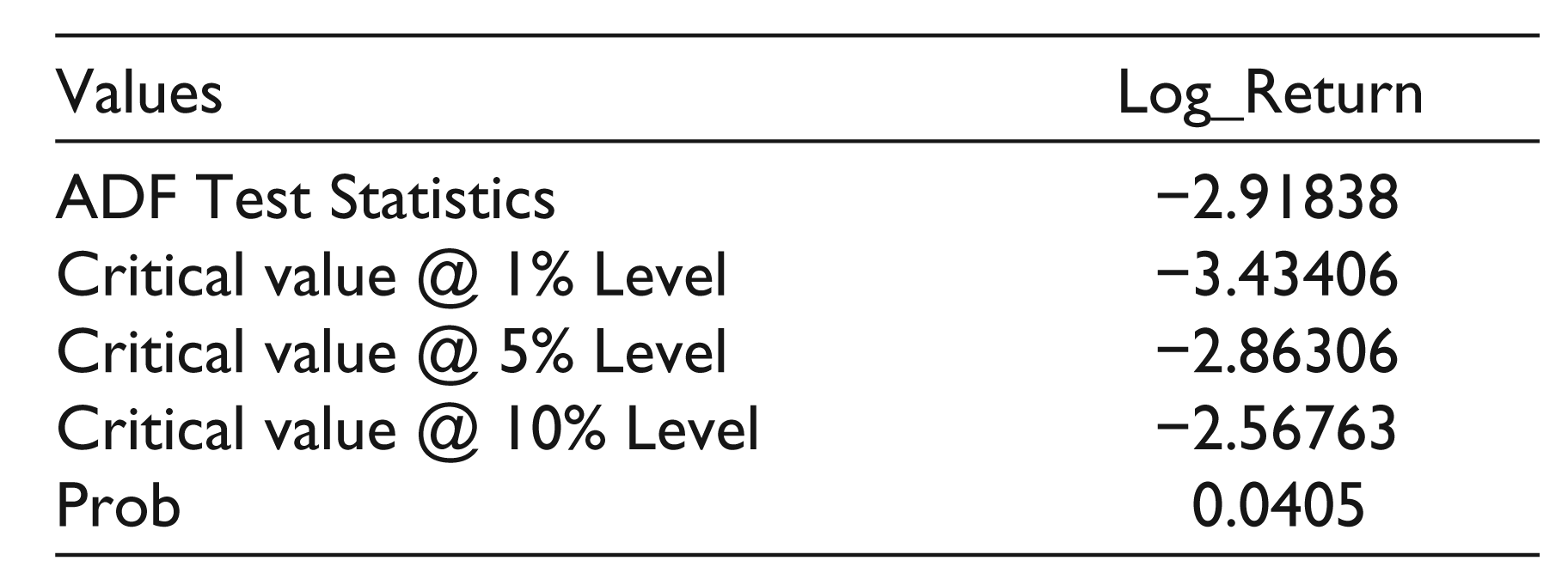
The term ‘stationary’ is a fundamental part of the time series econometric analysis. When using time series data for empirical financial research, it is imperative to check for stationarity of the data before any model is applied. A time series is said to be stationary if its joint probability, mean and variance do not change over time and it does not follow any trend. According to Dickey and Fuller (1979), a series is called stationary if its mean, variance and autocorrelation structure do not change over time and show no periodic fluctuations. If the series is not stationary, it is required to transform into a stationary series. An augmented Dickey–Fuller (ADF) test is used to check the unit root in a time series data. If the estimated ADF test statistics value is more than ADF critical values, it implies that there is unit root in the series and the series is not stationary. But if the estimated ADF test statistics value is less than ADF critical values, this means that the series is stationary. Table 1 represents ADF test for stationarity of the log values of the return series for a 30-min time frequency. The ADF test value is less than the critical values at a 10% level for return series; it is significant at a 10% level of significance, which means there is no unit root for return series.

Table 1.

30 Minutes: Augmented Dickey–Fuller Test for Stationarity of Log Return Series

Values	Log_Return
ADF Test Statistics	−2.91838
Critical value @ 1% Level	−3.43406
Critical value @ 5% Level	−2.86306
Critical value @ 10% Level	−2.56763
Prob	0.0405

Source: The authors.

Distributional Properties

Figure 1(a) reports the summary statistics of the return variable of the study for a 30-min time frequency. The summary statistics include mean, median, maximum and minimum values of the series. Standard deviation is the dispersion of the values from its mean; in this case, we can see the positive deviation in return series for the 30-min interval. In financial terms, standard deviation is used to measure risk involved in an investment instrument. The higher the dispersion or variability, the greater the standard deviation.

In financial analysis, normal distribution or Gaussian distribution is widely used in risk modelling and performance measurement. A distribution is said to be normally distributed when its mean, mode and median are equal and exactly half of the values are to the left of centre and exactly half the values are to the right. On the other side, the distribution of price variations (return) does not follow a simple random walk, and large fluctuations can be seen in stock markets. The skewness is a measure of asymmetry of the distribution. All symmetric distributions including normal distribution display skewness value equal to zero. As observed from Figure 1, return series has positive skewness, which implies that the right tail of the distribution is fatter than the left tail or that positive returns tend to occur more often than negative returns.

If a stock/index exhibits fatter tails than a normal distribution, then it displays excess kurtosis. Kurtosis is the shape of the distribution; it refers to the peakedness or flatness of a frequency distribution as compared to normal distribution. The standard normal distribution has a kurtosis of 3; so if the values are close to 3 that distribution is called mesokurtic distribution. If any distribution displays greater values than normal distribution, it is called leptokurtic distribution. And platykurtic distribution says the value is less than that of the normal distribution. In Figure 1(a), return series displays a leptokurtic distribution, that is, a fat-tailed distribution. The commonly used graphical method for analysing the tails of the distribution is the quantile-quantile (QQ) plot. Figure 2(b) displays the QQ plot of the return series; it can be observed that returns have fatter tails to fit the normal distribution.

Figure 1.

Source: The authors.

Dependence: Autocorrelation of Return

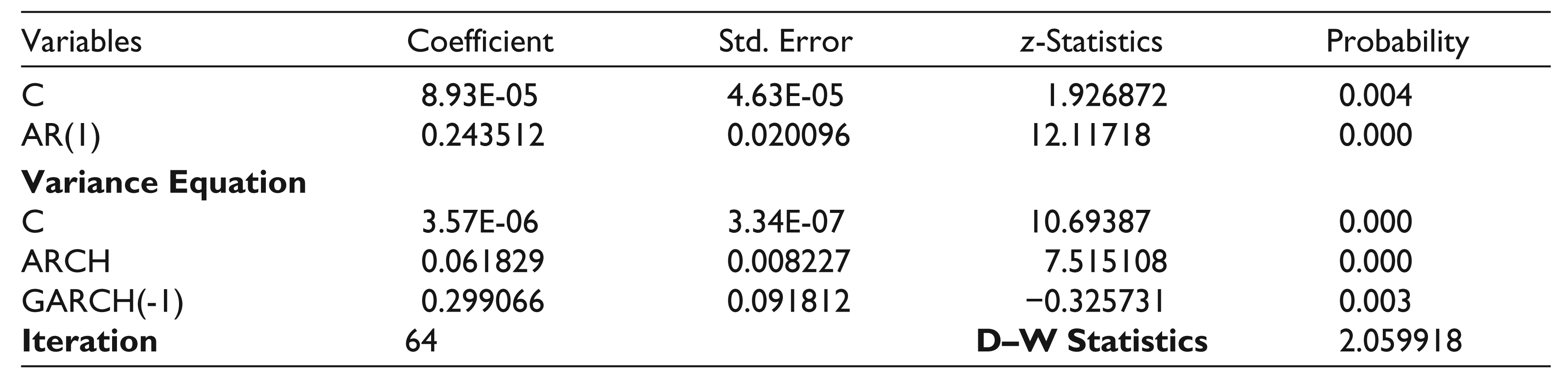
Autocorrelation, or serial correlation, is a mathematical representation of the degree of similarity between a given time series and a lagged version of itself over successive time intervals. Autocorrelation measures the relationship between a variable’s current value and its past values. In performance analysis, a positive first-order autocorrelation of period returns means that a positive (negative) return in one period will also be followed by a positive (negative) return in the next period. A negative first-order autocorrelation of returns means that a positive (negative) return in one period will be followed by a negative (positive) return in the next period. Chowdhury, Rahman, and Sadique (2015) revealed in an analysis that it is important to know the extent of autocorrelation and its underlying causes before any analysis. Schmid (2009) explains that the negative first-order autocorrelation of return is significantly stronger at a smaller time horizon (up to 3 minutes, which means between only few trades) and disappears at a longer time horizon like that of more than 30 minutes. Durbin and Watson (1951) have given the Durbin–Watson (D–W) statistics, which is a number that tests for autocorrelation in the residuals from statistical regression analysis. The D–W statistics is always between 0 and 4. If a value is close to 2, it means that there is no autocorrelation in the sample (see Table 2). Values approaching 0 indicate positive autocorrelation and values towards 4 indicate negative autocorrelation.

Figure 2 displays a visual inspection of volatility persistence from the correlogram of (a) absolute and (b) squared returns of the S&P CNX Nifty Futures Index for a 30-minutes time frequency for the first 36 lags. It provides an insight into the long memory characteristics of the volatility measure. In the figure, both absolute and squared returns show the significant correlation at the first and second lags followed by a correlation that is not significant, meaning slow decay of autocorrelation in returns. The pattern indicates a moving average term in the data.

Figure 2.

Source: The authors.

Heterogeneity: Volatility Clustering

Volatility clustering is the indication of shock persistence, that is, large movements/changes of either sign are followed by large movements/changes and small movements/changes follow small movements/changes. In volatility clustering, different measures of volatility display a positive autocorrelation over several days. The implication of volatility clustering is that volatility of many periods in future will be affected by present volatility shocks. Naik and Padhi (2015) empirically examined the high degree of volatility persistence across the BRIC markets. Figure 3 displays that price changes themselves occur in bunches rather than being evenly spaced over time.

Figure 3.

Source: The authors.

Clustered volatility is characterized by the ARCH model given by Robert F. Engle (1982) and GARCH by Bollerslev (1986). ARCH/ GARCH models consider the current error variance as a function of the previous period’s error variance.

The results of Table 2 show that ARCH and GARCH terms are statistically significant, but the sum of the ARCH and GARCH coefficient (0.061829 + 0.299066 = 0.360995) is below 1, which means that there is lack of persistence of volatility clusters over the sample period. And the impact of the previous period’s volatility GARCH term is much higher than the impact of the news about volatility from the previous period (ARCH term). The D–W value is around 2, which shows that there is no autocorrelation in the sample.

Table 2.

Volatility Modelling Through GARCH Model

Variables	Coefficient	Std. Error	z-Statistics	Probability
C	8.93E-05	4.63E-05	1.926872	0.004
AR(1)	0.243512	0.020096	12.11718	0.000
Variance Equation
C	3.57E-06	3.34E-07	10.69387	0.000
ARCH	0.061829	0.008227	7.515108	0.000
GARCH(-1)	0.299066	0.091812	−0.325731	0.003
Iteration	64		D–W Statistics	2.059918

Source: The authors.

Scaling

High-frequency data open the way for studying financial markets at different time scales, from minutes to years. For robust analysis, the scaling law is empirically found for a wide range of financial data and time intervals. A different time interval has been utilized for different studies. For some people, minute data are required (intraday traders), whereas for some studies 24 hours of scaled data are needed for analysis of the same stock (portfolio managers). Actually, there is no fixed time interval at which data should be analysed. It is totally dependent on the objective, requirement and the market. A lot of studies have empirically proven the existence of a scaling law in a wide range of financial data. Müller et al. (1990) analyse several million intraday FX prices and find scaling in the mean absolute changes of logarithmic prices, although the distributions vary across different time intervals. Dacorogna et al. (1993) observed similar hyperbolic decay of the autocorrelation function on daily returns. Johnson, Jefferies, and Hui (2003) list as a stylized fact that the probability distribution of price changes displays non-trivial scaling properties. Shakeel and Srivastava (2017), used high frequency 30 minutes time interval data to empirically gauge the volatility behavior of Indian future market.

Seasonality in Time Series Data

High-frequency financial time series data typically represent very strong periodic patterns or seasonality. Seasonality refers to the regular fluctuations in time series data over a certain period of time. Wachtel (1942) reported seasonality in stock returns for the first time. The seasonality can be found in trading volume, trade size, price and spread across different markets and time periods. Stock markets exhibit very strong seasonality in intraday data and intraweek data.

Intraday Trading Pattern

Stocks trade more frequently at the opening and closing time than during midday. In fact, if we plot the intraday trading pattern over the course of the day, we find that they typically follow a U-shaped pattern (Figure 4). The reason for the U-shaped pattern could be that at the beginning of the trading day all the information is well observed by the market overnight. The market participants made their trade strategies by analysing the available information for the coming day. At the opening (9:30 am), traders try to adjust their positions and prefer to wait till the middle (from 11:30 am to 2:00 pm) of the day, especially lunch time, to see the market trends, buyer and seller positions and activities. Just before closing (from 3:00 pm to 3:30 pm), all market participants make their final adjustments according to the information they received during the trade day, resulting in increased activity at the closing time.

Figure 4.

Source: The authors (based on Table A1).

Trade Size Distribution

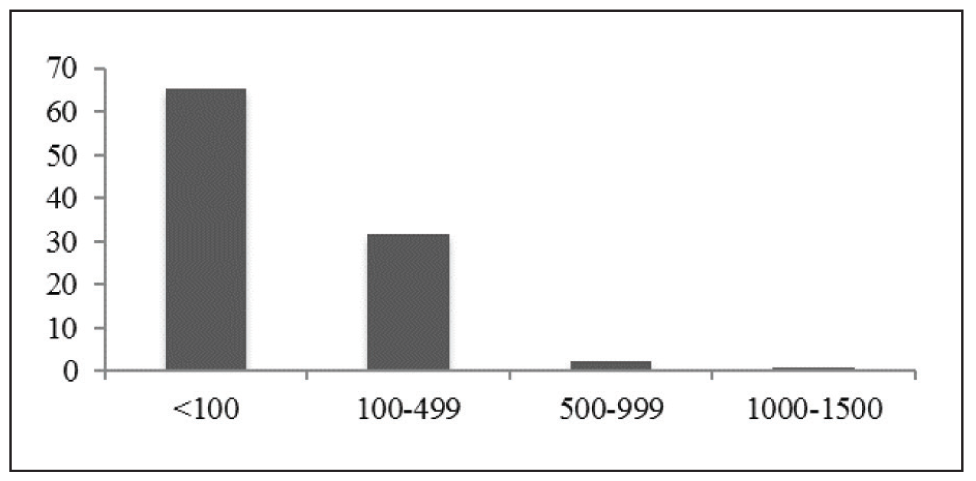
Average trade size is determined as the mean of all market trades over a historical period such as the last couple of days or last week. If we talk about pre-trade analysis for the traders, it is very important to know the trade size distribution. Figure 5 provides a summary of the percentage of execution that occurs at different trade sizes for futures index. It is clear from the figure that the vast majority of trades occur at relatively smaller sizes of 100 shares and 100–499 shares. Traders may utilize this information for making their trade decisions or they can go for smaller trade size transactions than the bigger one for better executions.

Figure 5.

Source: The authors (based on Table A2)

Price Trends

There is always a need to have an understanding about the recent activity or performance. In financial markets, informed investors or traders have the potential for extraordinary gains with concrete knowledge of price behaviour. Hence, traders or investors try to gauge the intraday price behaviour before investing. In Figure 6, intraday price trends have been captured. We found the W-shaped pattern for price in a day. It explains that at the opening time (from 09:15 am to 9:30 am) of the market, prices are on the higher side; then it starts showing downfall till 12 pm; afterwards, around 12:30 pm, there is again a peak and by closing time they are still on the higher side (from 3:00 pm to 3:30 pm), which gives us a W-shaped pattern for the intraday time period.

Figure 6.

Source: The authors (based on Table A1)

Effect-day of the Week

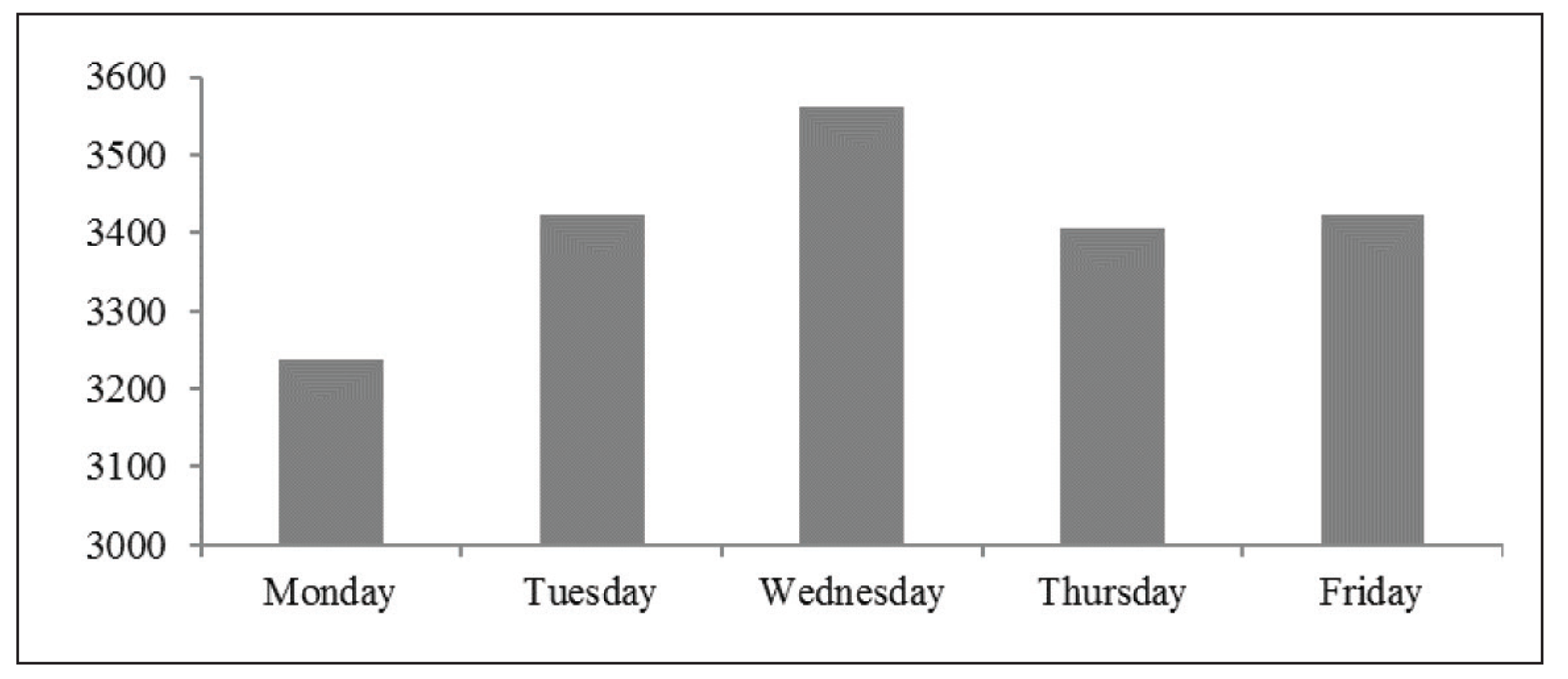
Day-of-the-week effect (also known as weekend effect or Monday effect) refers to the level of activity on different days of the week. Almost all exchanges are closed on weekends (Saturday and Sunday) and holidays, and therefore no trade takes place on these days. For weekdays, the level of activity is very different. In general, there is a minimum activity on Monday and maximum activities on the last working day (Friday). Cross (1973) found that the market tended to rise on Fridays and fall on Mondays. But in our case, maximum activity is found on Wednesday (midday of the working days) and minimum activity on Monday (Figure 7). The 2-day (Saturday and Sunday) inactivity periods, weekend announcements of earnings, executive changes and mergers and acquisitions lead to minimum activity or increased uncertainties on Monday. After Monday and Tuesday, which are active market days, Wednesday is found to be the most active day of the week; rumours settle after two days and investors try to take benefit of the information generated in the market after 2 working days. A similar day-of-the-week pattern has been found using daily prices also.

Figure 7.

Source: The authors (based on Table A3).

Spreads

Spread is the difference in price between the best bid and best ask. Basically, the bid–ask spread is the difference between the highest price that a buyer is willing to pay for an asset and the lowest price that a seller is willing to accept to sell it. Lower spreads are generally less difficult and less risky and higher spreads are more difficult and riskier. With the help of bid–ask spread, one can also determine the short-term trends. For example, if stocks sell at the bid price, it shows a negative trend of the market and on the other hand if the buyer is willing to pay the asking price, it shows the upward trend of the market. Figure 8 shows the trend of the spread across different intraday time periods. It is clear from the figure that at the opening time (9:15 am), the spread was maximum. After that, it started falling slightly, and at around 10:30 am, the bid–ask spread was at the lowest level. After 11:30 am, the spread showed no fluctuations and was stagnant till closing time.

Figure 8.

Source: The authors (based on Table A1).

Conclusion

Stylized facts of high-frequency data help us explain the market microstructure and make rational real-time decisions. Due to the increase in competition and demand for robust decision-making, it is need of the hour to use high-frequency data for analysis. Fortunately, significant progress has been made in recent years and numerous new theorems and techniques are being proposed. We observed that it is essential to be aware of the characteristics of empirical data before looking for the suitable model and for the analysis.

In this article, we have tried to show some light on the high-frequency financial time series data characteristics and the stylized facts using the S&P CNX Nifty futures index data. In the initial part of the study, we have tried to develop the understanding of the basic characteristics and facts of high-frequency data research and then through different observations, stylized facts of time series data have been presented using return series. The knowledge of such observations could be helpful to establish better empirical models for robust analysis. We discussed that stationarity as an essential feature needs to be achieved before analysing a financial time series. Time series data contain some unique distributional properties, which are able to explain the gain/loss asymmetry and shape of the distribution of the series. We found that the return series is positively skewed and shows leptokurtic distribution. The fundamental assumption for the modelled error term is that they should be uncorrelated, or we can say that there should not be autocorrelation. Slow decay of autocorrelation in return has been found, with significant correlation at the first and second lags followed by correlation that is not significant; this means there is no unit root present in the data. Through volatility clustering, we can explain that there is a lack of volatility persistence in the data of the sample period. High-frequency financial data typically present a very strong periodic pattern and seasonality. In this article, we have found the U-shaped intraday trading pattern and W-shaped intraday price pattern. And in day-of-the-week effect, it is interesting to find Wednesday to be the most active day of the week.

The study of such stylized facts helps to develop the understanding of the financial time series data and also could lay the foundation for nonlinear modelling and forecasting of financial returns. It is helpful to get acquainted with the empirical data before looking for the appropriate models of analysis.

Footnotes

Declaration of Conflicting Interests

The authors declared no potential conflicts of interest with respect to the research, authorship and/or publication of this article.

Funding

The authors received no financial support for the research, authorship and/or publication of this article.

Acknowledgements

The authors are grateful to the anonymous referees of the journal for their extremely useful suggestions to improve the quality of the article. Usual disclaimers apply.

Appendix

The following tables have been prepared by the author using high-frequency financial time series data of the S&P CNX Nifty futures for the period of June 2012–May 2013. Intraday time has been divided into 30-minute time intervals, and the average of every variable has been taken for each time interval, and for day-of-the-week effect (Table A3), average of the volume has been taken for each day. Table A1 represents intra day trading pattern (Figure 4), Price trends (Figure 6) and Spreads (Figure 8), Table A2 represents trade size distribution (Figure 5) and Table A3 is prepared for day of the week effect (Figure 7) in the seasonality of time series data.

References

Andersen

T. G.

, Bollerslev

, Diebold

F. X.

, & Labys

(2003). Modelling and forecasting realized volatility. Econometrica, 71(2), 579–625.

Bollerslev

(1986). Generalized autoregressive conditional heteroskedasticity. Journal of Econometrics, 31(3), 307–327.

Chowdhury

S. S. H.

, Rahman

M. A.

, & Sadique

M. S.

(2015). Behaviour of stock return autocorrelation in the GCC stock markets. Global Business Review, 16(5), 737–746.

Cross

(1973). The behavior of stock prices on Fridays and Mondays. Financial Analysts Journal, 29(6), 67–69.

Dacorogna

, Gencay

, Muller

, Olsen

, & Pictet

(2001). An introduction to high frequency finance. Academic Press.

Dacorogna

M. M.

, Müller

U. A.

, Nagler

R. J.

, Olsen

R. B.

, & Pictet

O. V.

(1993). A geographical model for the daily and weekly seasonal volatility in the foreign exchange market. Journal of International Money and Finance, 12(4), 413–438.

Dickey

D. A.

, & Fuller

W. A.

(1979). Distribution of the estimators for autoregressive time series with a unit root. Journal of the American statistical association, 74(366a), 427–431.

Durbin

, & Watson

G. S.

(1951). Testing for serial correlation in least squares regression. II. Biometrika, 38(1/2), 159–177.

Engle

R. F.

(1982). Autoregressive conditional heteroscedasticity with estimates of the variance of United Kingdom inflation. Econometrica: Journal of the Econometric Society, 50(4), 987–1007.

10.

Engle

R. F.

, & Russell

J. R.

(1998). Autoregressive conditional duration: A new model for irregularly spaced transaction data. Econometrica, 65, 1127–1162.

11.

Engle

R. F.

, Lilien

D. M.

, & Robins

R. P.

(1987). Estimating time varying risk premia in the term structure: The ARCH-M model. Econometrica: Journal of the Econometric Society, 55(2), 391–407.

12.

Goodhart

C. A.

, & O’Hara

(1997). High frequency data in financial markets: Issues and applications. Journal of Empirical Finance, 4(2–3), 73–114.

13.

Johnson

N. F.

, Jefferies

, & Hui

P. M.

(2003). Financial market complexity. Oxford: Oxford University Press.

14.

McInish

T. H.

, & Wood

R. A.

(1992). An analysis of intraday patterns in bid/ask spreads for NYSE stocks. The Journal of Finance, 47(2), 753–764.

15.

Müller

U. A.

, Dacorogna

M. M.

, Olsen

R. B.

, Pictet

O. V.

, Schwarz

, & Morgenegg

(1990). Statistical study of foreign exchange rates, empirical evidence of a price change scaling law, and intraday analysis. Journal of Banking & Finance, 14(6), 1189–1208.

16.

Naik

P. K.

, & Padhi

(2015). Stock market volatility and equity trading volume: Empirical examination from Brazil, Russia, India and China (BRIC). Global Business Review, 16(5_suppl), 28S–45S.

17.

Nelson

D. B.

(1991). Conditional heteroskedasticity in asset returns: A new approach. Econometrica: Journal of the Econometric Society, 59(2), 347–370.

18.

O’Hara

(2015). High frequency market microstructure. Journal of Financial Economics, 116(2), 257–270.

19.

Russell

J. R.

, & Engle

R. F.

(2010). Analysis of high-frequency data. In Handbook of financial econometrics: tools and techniques (pp. 383–426). North-Holland.

20.

Schmid

Friedrich

(2009). High frequency financial markets data cleaning and stylised facts in financial markets data. Seminar of Economic and Social Statistics, University of Cologne.

21.

Shakeel

, & Srivastava

(2017). Analysis of intraday volatility using high frequency data: An empirical investigation of Indian futures market. Al-Barkaat Journal of Finance & Management, 9(2), 29–45.

22.

Wachtel

S. B.

(1942). Certain observation on seasonal movement in stock prices. Journal of Business, 15(2), 184–193.