



Abstract
This study aims to forecast air passenger and cargo demand of the Indian aviation industry using the autoregressive integrated moving average (ARIMA) and Bayesian structural time series (BSTS) models. We utilized 10 years’ (2009–2018) air passenger and cargo data obtained from the Directorate General of Civil Aviation (DGCA-India) website. The study assessed both ARIMA and BSTS models’ ability to incorporate uncertainty under dynamic settings. Findings inferred that, along with ARIMA, BSTS is also suitable for short-term forecasting of all four (international passenger, domestic passenger, international air cargo, and domestic air cargo) commercial aviation sectors. Recommendations and directions for further research in medium-term and long-term forecasting of the Indian airline industry were also summarized.
Introduction
In recent times, business organizations are facing numerous challenges and uncertainty. It is crucial for companies to make the right decisions in the changing business world, as decision-making plays a significant role and affects the company’s business extensively. Hence, the top management should be prudent in making strategic moves based on their decisions. The companies must be more diligent while considering several factors for their decision-making. Among those, past observations always play a crucial role in making decisions. There are several statistical forecasting techniques from univariate to multivariate that use past observations to predict the future. In real time, these past observations are used in the business world for predicting demand, sales, inventory, growth and so on. Also, the past observations are used by policymakers at a macro level for predicting and decision-making to determine the economic growth of the nation. The aviation sector is one of the most challenging industries to apply predictive analysis. However, there is limited research in academia with a special focus on developing appropriate forecasting techniques to predict the demand and growth of the airline industry. Hence, this study focused on the Indian airline industry and attempted to forecast the airline passenger and air cargo demand. The reason for selecting the Indian aviation sector is, in 2018, the Indian airline industry ranked 5th in the world in passenger transport and 17th in freight carriage (World Bank, n.d.). Also, it is expected to rank third in the world in overall air transport by 2024 (International Air Transport Association, 2018). Though the industry has grown substantially in the twenty-first century, to the best of the authors’ knowledge, there is limited research in academia to develop more appropriate models to predict the growth of the Indian airline industry. So, beginning at macro-level predictions would be a good starting point for researchers to pursue further in the above-said research area. Hence, to fill the gap in the literature and to instigate further research, this study aims to do short-term forecasting of the airline passenger and air cargo carried by using the popular statistical forecasting models, namely autoregressive integrated moving average (ARIMA) and Bayesian structural time series (BSTS). ARIMA is one of the most commonly used classical forecasting methods, and Bayesian method of analysing time series data is an ever-growing field (Steel, 2010). These models were compared based on their forecasting performance and accuracy, which would also assess the suitability of the models in short-term forecasting of the airline industry. The following sections present the literature review, objectives, rationale of the study, methodology, data analysis and results, discussion, conclusion, managerial implications, limitations and future research directions.
Literature Review
Time series data play a vital role in forecasting for management decisions. The time-series data help to understand the trend, seasonality and growth rate. The different forecasting models enable the researchers to estimate the forecast error for analysing the accuracy of the forecast. Several studies have used forecasting models to predict airline passenger and air cargo demand. The study by Alekseev and Seixas (2002) forecasted the air transport demand in the Brazilian industry, and the study found that neural networks are capable of outperforming traditional econometric approaches that can accurately generalize the time series behaviour in reality. BaFail (2004) forecasted domestic and international air passengers in Saudi Arabia by using neural networks. The authors also indicated the factors that affect the number of air passengers. Ahmadzade (2010) predicted the air passenger in an international airport, and the time series data were tested for stationarity using the augmented Dickey–Fuller (ADF) test. Chen et al. (2012) forecasted the air passenger and air cargo by using back-propagation neural networks. The authors found the factors influencing air passenger and air cargo demand, and they found the forecasting accuracy by using the mean absolute percentage error (MAPE). The authors Srisaeng et al. (2015) predicted Australia’s domestic air passenger demand using first-time genetic algorithms. They proposed and analysed the algorithms by dividing the dataset into training and testing sets. They evaluated the model fit and accuracy by using mean absolute error (MAE), MAPE, mean squared error (MSE), and root mean squared error (RMSE). However, they indicated the fitness and accuracy by using the results of MAPE. Kim and Shin (2016) forecasted the short-term air passenger demand by using big data from search engine queries for identifying short-term fluctuations. Mohie El-Din et al. (2017) predicted the air passenger demand by using back-propagation neural networks and genetic algorithms. In their study, they identified and analysed the factors influencing air passenger demand, and also analysed the forecasting performance. Olaniyi et al. (2018) estimated the domestic air passenger demand in Nigeria by using a single moving average and simple exponential smoothing method. They also utilized mean square deviations to compare the forecast accuracy of the model. They indicated that 2 years single moving average is closer to the original data than the exponential smoothing method. The study by Sharma et al. (2018) forecasted air passengers by using an exponential smoothing method. However, there are studies in the field, which used traditional multiple regression to modern machine learning techniques for time series forecasting.
Various studies also employed ARIMA and seasonal autoregressive integrated moving average (SARIMA) for forecasting air passengers. Bao et al. (2012) predicted the air passenger traffic by proposing a model named ensemble empirical mode decomposition (EEMD)-based support vector machines (SVMs). The results of the study revealed that the proposed EEMD model outperformed the counterpart models such as single SVMs, ARIMA, and Holt-Winter model in terms of forecast accuracy measures, that is, RMSE and MAPE. Bougas (2013) forecasted air passenger traffic flows by using time series models. The author utilized the forecasting models, namely, harmonic regression, Holt-Winters exponential smoothing, ARIMA and SARIMA. The study results indicated that all the models produced accurate results in forecasting with MAPE, and root mean square percentage error (RMSPE) scores were below 10 per cent on average. A study by Robertson & Wallin (2014) predicted the monthly air passenger flow from Sweden. The authors compared the Naive model and Causal model (termed as SARIMA in the study). The study concluded that the SARIMA model outperformed with the lower MAPE values that are essential for a good model fit. Ming et al. (2014) predicted air passenger traffic by using a hybrid ARIMA–SVM model. Their study indicated the superiority of the model in time series prediction. Nieto and Carmona Benitez (2015) utilized the auto regressive integrated moving average (ARIMA)-generalized autoregressive conditional heteroskedasticity (GARCH)-bootstrap method to forecast the air passenger demand, and their study indicated that ARIMA–GARCH–bootstrap method outperformed over other methods like Grey model and ARIMA model. Xu et al. (2019) used SARIMA–SVR (support vector regression) model to forecast short-term demand in China’s aviation industry. Their research benchmarked with Ruiz-Aguilar et al. (2014) similar hybrid approach based on SARIMA and artificial neural networks (ANN). The authors’ Xu et al. (2019) used a novel approach by including Gaussian White noise into the model and forecasted statistical indicators in the aviation industry. Their research results revealed that incorporating the Gaussian white noise into the models would increase the forecasting accuracy. Marazzo et al. (2010) investigated the air transport demand and economic growth in Brazil by considering the 40 years of data (1966–2006). The authors gave special focus on stationary features and long-run equilibrium in a vector autoregressive environment. They used (a) unit-root and cointegration tests, (b) error correction model, impulse-response function and variance decomposition and (c) Granger causality tests. Their study results revealed that air transport demand and economic growth time series is first difference stationary and cointegrated; also, there is a long-run equilibrium relationship between the variables.
To the best of the authors’ knowledge, there is minimal academic research on forecasting air passenger and air cargo demand within the Indian context. Rengaraju and Tamizh Arasan (1992) developed a city-pair model for forecasting domestic air travel demand, and they used multiple regression analysis. The research was limited to micro-level analysis of airline industry demand and the approach was found useful in city-pair-wise demand forecasting. Basak et al. (2013) forecasted air cargo growth in India by using double exponential smoothing and trend analysis along with econometric analysis. The research focused only on air cargo sector. A study by Srinidhi and Manrai (2014) analysed the international air transport demand by using regression, time series analysis (Holt’s Exponential Smoothing), and two demand drivers’ econometric model. The forecasts were made for 7 years until 2020. The research focused on predicting international air transport demand between major US metropolitan cities and India is one of the well noticeable long-haul air transport research in the Indian aviation sector context.
This research, novel in its concept, covers the macroscopic view of all four major sub-sectors of the commercial aviation industry, that is, domestic passenger, international passenger, domestic cargo and international cargo. Though various methods were used by researchers to forecast/nowcast the airline industry demand, all have their own limitations because airline industry growth is also influenced by various other external factors such as Government policies, new airport development, International treaties, and so on. However, when it comes to short-term forecasting, the selection of variables depends on the objective of the research. The single variable that is, the number of pax (passengers)/tons of cargo carried, can be used for short-term forecasting (International Civil Aviation Organization, 2006).
Objectives of the Study
The major objective of the study is to compare and test the accuracy of the classical ARIMA model and emerging BSTS models in short-term forecasting of all four Indian civil aviation sectors—international passenger, domestic passenger, international cargo, and domestic cargo using monthly time-stamped data.
Rationale of the Study
Studying aviation industry growth is a complex process. It varies from individual passenger experience (Majra et al., 2016)/satisfaction (Sarkar & Baisya, 2005) to macro-level multivariate machine learning forecasting. Due to the rapid growth of the aviation industry all around the World, there were several developments in forecasting techniques for the broad application in various sectors of aviation planning. But forecasting accuracy still remains as a challenge. International Civil Aviation Organization (2006) has developed a manual that presented the techniques that are widely available and used for air traffic forecasting. They broadly classified the existing techniques into three categories, namely quantitative, qualitative and decision analysis. The quantitative forecasting methods included the time series analysis, causal methods and econometric methods. The qualitative forecasting methods included the Delphi technique and technological forecasting, whereas the decision analysis includes market research, industry surveys, probabilistic analysis, Bayesian analysis and system dynamics. The air traffic forecasts help to address the important issues of facility planning and financial planning, which includes the terminal capacity, cargo facilities, and airport infrastructure and development. However, these are planned only through short-term forecasting. It is stated that air traffic forecasting in India is based on quantitative, qualitative and decision analysis. Mostly, they use the econometric model, linear trend projection and exponential trend projection. However, the Directorate General of Civil Aviation (2011) called for expression of interest for developing a new model to forecast air traffic as the forecast for international traffic to/from India are based on trend analysis usually carried out by Air India and Airports Authority of India, which is also supplemented by the annual country forecast by aircraft manufacturers and IATA. Hence, developing an appropriate model for forecasting air passenger and cargo for the Indian aviation industry is a need of the hour, and the rationale behind this study is to do short-term forecasting of the demand of Indian airline industry by using two most appropriate methods, that is, classical ARIMA and emerging BSTS with short monthly time-stamped data for the period from 2009 to 2018. According to the International Civil Aviation Organization (2006) ‘Manual on Air Traffic Forecasting,’ the first step in forecasting air traffic is to study the time series using historical data. Also, the manual recommends using either ARIMA or simpler methods such as exponential smoothing/Holt-Winters method for short-term forecasting (1 year).
Methodology
The 10 years’ (2009–2018) annual data of commercial Aviation sectors in India was obtained from DGCA (Directorate General of Civil Aviation, n.d.) official website. The four segments of data obtained from DGCA, that is, domestic air passengers, international air passengers, domestic air cargo, and international air cargo are independent in nature. The data encompass the actual information on the total number of domestic and international airline passengers and domestic and international air cargo carried in the past 10 years. The data accounted for 120 observations each in domestic and international airline passenger and air cargo, that is, a total of 480 observations of 120 each.
Various univariant and multivariant forecasting models and methods are available in the literature; the availability of data and its suitability to meet the research objectives are the major factors for the selection of appropriate methods (Nieto & Carmona Benitez, 2015). Also, according to International Civil Aviation Organization (2006), time series analysis/trend analysis can be done with ‘air traffic data in terms of the number of passengers/tonnes of freight’ and ‘time’ for short-term forecasting. Since this research is aimed to project the overall growth of the airline industry in India covering all four segments, the classic Box et al. (1976) approach of univariate analysis for forecasting demand was adopted. Hereinafter, the current study examined the appropriate method for short-term forecasting of airline passenger and air cargo by using two popular methods, that is, ARIMA and BSTS.
First, the data were converted into time series data using the ‘stats’ package, which is part of R (R Core Team, 2019). Further, the time series data were analysed by using ARIMA modelling, while it is also tested for its stationarity by employing Augmented–Dickey Fuller (ADF) unit root tests. Second, the best ARIMA model (P, D, Q) was identified by its implied low Akaike information criterion (AIC) condition along with its forecasted data for the year 2020. Third, the simple BSTS modelling was utilized to make forecasting for the same set of data. Finally, both models are compared based on their efficiency in forecasting, and the ability to incorporate uncertainty was reported under appropriate sections. The comprehensive R archive network (CRAN) packages of ‘tseries’ (Trapletti & Hornik, 2019), ‘forecast’ (Hyndman & Khandakar, 2008; Hyndman et al., 2019), ‘bsts’ Scott (2019) and ‘ggfortify’(Horikoshi & Tang, 2016; Tang et al., 2016), ‘dplyr’ (Wickham et al., 2019), ‘ggplot2’(Wickham, 2016), ‘dygraphs’ (Vanderkam et al., 2018) packages for data visualization were used in Rstudio (RStudio Team, 2018) for data analysis.
Autoregressive Integrated Moving Average
The term ‘ARIMA’ represents the autoregressive integrated moving average. It is a statistical model that analyses the time series data for forecasting. The ARIMA model was popularized in the textbook Time Series Analysis: Forecasting and Control by George Box and Gwilym Jenkins in the year 1970. They also came up with the solution for non-stationary data, whereas they indicated how non-stationary data could be made stationary by ‘differencing’ the series (Box & Jenkins, 1970). The term ‘ARIMA’ was interchangeably used as the ‘Box-Jenkins Model’ by the researchers. Stellwagen and Tashman (2013) also claim that other forecasting methods outperform over ARIMA models in practice concerning forecasting accuracy. They suggested that forecasters should take into consideration for switching into different methods for different data instead of following a one-size-fits-all approach.
The ARIMA model is typically expressed by (p, d, q), where p captures the Autoregressive part, d represents the integrated, and q denotes the moving average part of ARIMA. Technically, p indicates the number of lagged values, d indicates the number of times the data has differenced (if d = 0, means the data are already stationary, and it implies ARMA, not ARIMA), and q denotes the number of lagged values for error term (Abugaber, n.d.). Usually, the non-seasonal ARIMA model is expressed as ARIMA (p, d, q), that is, p-the order of AR, d-the order of differencing, and q-the order of MA. The seasonal ARIMA model is denoted as ARIMA (p, d, q) * (P, D, Q), where p, d, q indicates the order of short-term components and P, D, Q denote the seasonal components of the model (Stellwagen & Tashman, 2013). More specifically, in seasonal ARIMA model, P denotes the number of seasonal autoregressive (SAR), D denotes the number of seasonal differences, and Q denotes the number of seasonal moving averages (SMA).
The formula for the basic forecasting model formula by Box and Jenkins is expressed below (Abugaber, n.d.). However, the original Box and Jenkins convention use the negative signs in the MA part. Most of the software use positive sign, including R package, although there is no ambiguity (Nau, 2005).

Stationarity of the Data
The stationarity of the data implies the condition that the mean, variance and covariance of the data are constant over a period without any fluctuations. Hence, the underlying assumption for the time series analysis is the stationarity of the data. If the data are non-stationary, the stationarity could be achieved by the differencing approach proposed by Box and Jenkins.
Determining Stationarity (Through Differencing)
If d = 0

For first-order difference, if d = 1

Similarly, it goes on with several times of differencing that is required by the model. However, the Box and Jenkins (1970) model procedures involve three steps, namely model identification/selection, parameter estimates and model checking, including residual diagnostics and Ljung Box test. Later developments in the model lead to the identification of the best fit models based on the AIC (Hyndman & Khandakar, 2008).
Ord and Lowe (1996) indicated that most of the software packages use inbuilt algorithms to automatically select the best model of ARIMA, which outperforms the manual selection approaches proposed by Box and Jenkins. In this study, the ARIMA model was identified using the R software. The best fit model was estimated by R based on the low AIC. The ARIMA model was estimated using the inbuilt algorithms in R. This study adopted five steps to identify the best fit model, respectively. The ARIMA modelling procedure was adopted in this study as follows: (a) Exploratory Data Analysis, (b) decomposition of Data, (c) test the stationarity, (d) fit a model using automated algorithms, (e) residual diagnostics and (f) estimate the forecast and evaluate its accuracy (Elprince, 2014; Kimnewzealand, 2017; Larsen, 2016; DeWitt, 2018).
Bayesian Structural Time Series
The BSTS is a machine learning technique proposed by Scott and Varian (2012 & 2013), which is used for time series forecasting, nowcasting and inferring causal impact. This approach encompasses all the three statistical methods, such as Kalman filters, Spike and Slab regression, and Bayesian model averaging into an integrated system termed as BSTS. The system was developed for nowcasting Google’s trends data for several possible applications. The Bayesian methods forecast well under uncertainty conditions (Scott & Varian, 2012). The BSTS model and the bsts R package can handle the non-Gaussian data, are more appropriate for long-term forecasting and support multiple seasonalities (Scott, 2017). BSTS model is more transparent than the ARIMA model, which does not rely on the lags, differencing and moving averages; instead, it handles uncertainty more efficiently. The BSTS model enables researchers to calculate posterior uncertainty, control the variances, and impose prior beliefs. The BSTS structural model equation is given below (Larsen, 2016):


Data Analysis and Results
The main aim of this study is to forecast domestic and international airline passengers, and air cargo carried. The four sets of data with 120 observations were considered for the study. Both the ARIMA and BSTS models were estimated to analyse the forecasting performance and accuracy.
The stationarity has become the underlying assumption for carrying out time-series analysis. The concept of stationarity is meant as the statistical properties of the time series do not change over time. However, it does not mean that the series does not change over time; instead, the way it changes does not change over time (Palachy, 2019). However, it is more common to have air passenger data as non-stationary series. For the ARIMA model, if the data are non-stationary, the differencing technique must be used to achieve stationary of the data, as suggested by Box and Jenkins (1976). There are alternative ways to analyse the stationarity of the data, it could be analysed using either unit root tests or autocorrelation (ACF).
Results of ARIMA model (for India International Air Passengers)
The ARIMA modelling procedure was adopted in this study as follows (Elprince, 2014; Kimnewzealand, 2017; Larsen, 2016; DeWitt, 2018). Based on the recommendations from the authors, appropriate procedures were included in this study concerning the characteristics of the airline passenger data. All procedures were performed with R packages:
Exploratory data analysis Decomposition of data Test the stationarity Fit a model using automated algorithms Residual diagnostics Estimate the forecasts and evaluate its accuracy
In the first step, India’s international and domestic air passengers and air cargo carried (raw data) were imported and plotted in the graph (Figures 1 and 2) using base plot function to understand the seasonal effects, if any. It is understood from the figure that there is a seasonal variation throughout the given time with fluctuations. Hence, it implies that the data are non-stationary. Further, it would be taken to the next step to test the stationarity statistically.


Descriptive Statistics
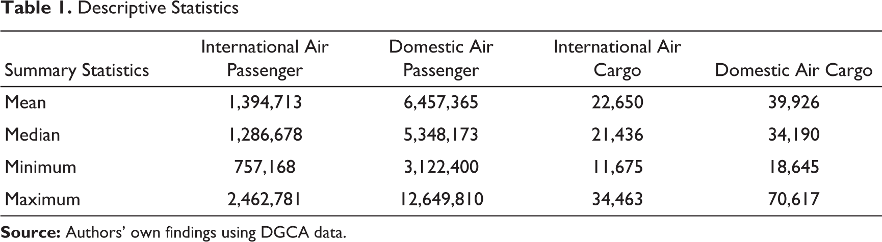
Based on the minimum and maximum values in the below Table 1, it is understood that there is an increase in international and domestic air passenger and air cargo flow from the period 2009 to 2018. The overall mean also resulted in high, and there is a noticeable increase in domestic air passenger and air cargo when compared to the international air passenger and air cargo. However, the data are non-stationary as it is prevalent in the airline industry due to the trend and seasonal effects.
The decomposition of time series data has been done to understand the estimates of trend, seasonal and random components. The process of including seasonal indexes for removing the seasonal effects from a time series is referred to as deseasonalizing the time series (Anderson et al., 2019). The time series were deseasonalized by using a Multiplicative decomposition model, which is written as yt = S t T t ε t where S t denotes the seasonal trend, T t denotes the overall trend, and εt denotes the unexplained noise (in the figure, it is mentioned as remainder). Firstly, the time series data were plotted seasonally to understand the underlying seasonal patterns/variations over time (Figures 3–6).

From Figure 3, monthly seasonal plot, it can be noted that there is a sharp rise in international air passenger arrivals in the month of December. This may be due to the new year holidays, whereas an apparent fall was observed during the months of February and September. Hence, for the International air passenger segment, December is the peak season; February and September are low seasons, whereas all other months remain as average without many fluctuations in the seasonal trend. Figure-4—monthly seasonal plot—indicates the monthly domestic air passenger trend. From Figure 4, it is inferred that May and December are the peak seasons and February is low season for the domestic air passenger market. The reason for the peak season trend may also be the educational vacations and other seasonal holidays. Hence, it is concluded that December is the peak season, and February is low season for both domestic and international air passenger traffic, whereas May month is also the peak season for domestic air passenger traffic.


From Figure 5 (Seasonal plot—International Air Cargo), the carriage of cargo in tons has seen a significant rise since December 2016. The years 2017 and 2018 have witnessed the strongest growth. There is no seasonal difference in the carriage of International cargo in the months of March-December, whereas relatively low growth is noticed in the month of February and noticeable growths in the months of September–October throughout the 10 years of study. In the domestic Air cargo segment (Figure 6), there was no noticeable seasonable difference till 2015, whereas, since 2016, the air cargo carried in the months of January–February was relatively low and the months of September–October have seen a relatively high carriage.


Figures 7–10 help to understand the time series decomposition of the trend, seasonal, noise. It is evident that the data are non-stationary (contains random walks) due to their linear trend and seasonal effects.
In this study, the stationarity of the time series data was tested using the ADF test (Dickey & Fuller, 1981). The ADF test was performed using the ADF test function from the tseries R package. It uses the differencing approach by using the first difference of the time series against the series lagged k times. According to the ADF test, if the null hypothesis is accepted, the data are non-stationary.
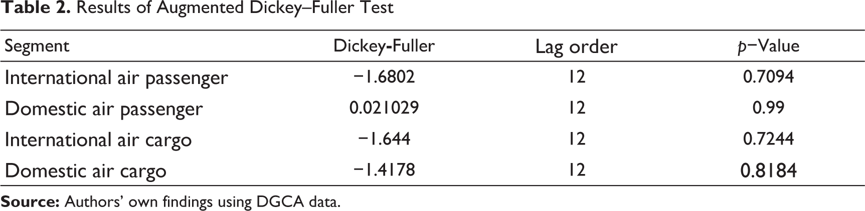
The p-value of the ADF test is greater than 0.05 (Table 2), which fails to reject the null hypothesis. Hence, the results of the ADF test indicate that the time series data are non-stationary. Further, it is required to make the data stationary. Hence, first-order differencing could be utilized to remove the trends and seasonal effects.
Results of Augmented Dickey–Fuller Test
This step enables us to identify and estimate the model with the appropriate values for p, d, and q, which represents the AR part, degree of differencing, and MA part. For this, the auto. Arima function is used in R. Another way could be used to identify the best model by including trace=true to the auto. Arima function, where the set of models would be displayed, and the best model could be identified by comparing the low values of the AIC. Moreover, in this study, the best model was identified and estimated automatically using auto. ARIMA function of forecast package (Hyndman & Khandakar, 2008; Hyndman et al., 2019).
From Table 3, the ARIMA model for the International air passenger data identified the order of the model as ARIMA(0,1,0)(0,1,1){12} (ARIMA (p, d, q)*(P, D, Q)(m)), whereas for the domestic air passenger the order of the model was identified as ARIMA(0,1,1)(0,1,1){12} (ARIMA (p, d, q)*(P, D, Q)(m)) resembling an seasonal random trend model. The model was estimated with first-order differencing with d = 1. Hence, the model is identified as a SARIMA for the air passenger, as there is a seasonal effect every year. The ARIMA model was predicted with the same order for the series and depicted in the Figures 11 and 12, respectively. The model was forecasted until 2020.
The ARIMA model for the International air cargo data identified the order of the model as ARIMA(1,1,0)(2,0,0){12} (ARIMA (p, d, q)*(P, D, Q)(m)), whereas for the domestic air cargo the order of the model was identified as ARIMA (4,1,0)(2,0,0){12} (ARIMA (p, d, q)*(P, D, Q)(m)). The model was estimated with first-order differencing with d = 1. Hence, the ARIMA model identified for air cargo is without moving averages. The ARIMA model was predicted with the same order for the series and depicted in the Figures 13 and 14, respectively. The model was forecasted until 2020 without using log transformation.
Next, the prediction intervals of the 95 per cent confidence level were computed (Refer to Figures 15–18). The black colour indicates the actual values; the red line indicates the forecasted values, whereas the blue line indicates the error bounds of confidence intervals at 95 per cent.
Results of ARIMA Model


Autocorrelation function
Figures 19–22 depict the ACF of the residuals. The ACF of the residuals shows the correlations between the series xt and the series of lags xtt-1, xt-2, xt-3, and so on. It is found that there is no significant correlation for any lags, which indicates the good ACF condition for residuals. Hence, there are no significant autocorrelations.
Partial autocorrelation function
Figures 23–26 show the partial autocorrelation function (PACF) of the residuals. The PACF of the residuals shows the extent of the lags. It helps to analyse the appropriateness of the lags in the AR part or all the three parts (p, d, q) of the ARIMA model.
Q–Q plot
The below Figures 27–30 show the Q–Q plot; it is found that there is no pattern in the residuals. Here, the ARIMA model used the maximum likelihood estimation, and the figure indicates that the data are normally distributed, which supports the assumption.
Test of stationarity
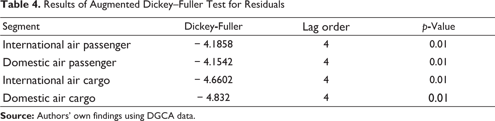
Finally, the ADF test was used to verify the stationarity of the time series. The p-value of less than 0.05 (Table 4) indicates that the residuals of time series are stationary, which rejects the null hypothesis. Hence, the prediction model is stationary.


Results of Augmented Dickey–Fuller Test for Residuals
Figures 31–34 show the ARIMA model, including the essential characteristics of first-order differencing, seasonal differencing. In order to validate the model, the year 2018 has been considered as a holdout period, and the log transformation was used to decompose and model the growth rate.
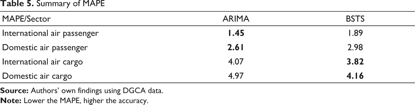
The MAPE measure was used to evaluate the forecast accuracy. The MAPE is the most commonly used accuracy measure statistics, which is easier to understand than other measures. It expresses accuracy in terms of percentage error. If the MAPE values are smaller, it indicates a better fit (Minitab Express, n.d.). In research by Xu et al. (2019) suggested that over forecasting may affect the resources and profits, whereas under forecasting may lead to a reduction in service levels. Hence, the best model could be identified using lower MAPE values. The ARIMA-Holdout MAPE value for International air passenger is at 1.45 per cent, Domestic air passenger is at 2.61 per cent, International Cargo is at 4.07 per cent, and Domestic Cargo is at 4.97 per cent. Hence, this model is considered a good fit with smaller values less than an average of 5 per cent. The forecast is off by 1.45 per cent, 2.61 per cent, 4.07 per cent, and 4.97 per cent, respectively.


The Bayesian Structural Time Series Model
A BSTS model can decompose the trend and regression components (Scott & Varian, 2012). The BSTS model can accommodate non-stationary data for time series forecasting. Larsen (2016) stated that BSTS is more suitable for forecasting values with greater accuracy with limited observations. Some studies compared ARIMA and BSTS in different research settings. Spedding and Chan (2000) proposed a Bayesian dynamic linear time series model as an alternative technique for demand forecasting in a dynamic environment. The authors compared the Bayesian dynamic linear time series model with the classical ARIMA model. Kitamura (2018) forecasted Japan’s spot liquefied natural gas (LNG) prices using the BSTS and found that the BSTS model outperformed the ARIMA model in the short-term forecasting. However, the ARIMA model has smaller errors. Also, the author found that the BSTS model with regression components outperform a single BSTS model for long-term forecasting. However, this study considered the air passenger and air cargo data, without any regressors using the BSTS model (Brodersen et al., 2015; Scott & Varian, 2012, 2014; Varian, 2014) to do short-term forecasting. Hence, the simple BSTS model was run with the BSTS package and codes suggested by Scott (2018) and Larsen (2016) using log10 transformation, Markov chain Monte Carlo (MCMC) Iterations and burn-in. The air passenger data is usually non-stationary, so log10 transformation was used to stabilize the variance and improve forecasting accuracy. The log transformation will also make the model multiplicative, which is appropriate for the used data. Liu et al. (2016) stated that several factors affect the essential number of MCMC draws, namely (a) the desired relative precision (d) which is set as 0.01 and 0.005, (b) confidence level (1−α), which is 0.9 and 0.95, and (c) tail probability (p), which is 0.8, 0.9, and 0.95.
Further, the BSTS forecasts are done for the period 2009 to 2019. The year 2018 was used as a holdout period for evaluation in order to observe the forecasting performance of the model with the actual versus forecasted values. The Kalman filtering and MCMC draws were utilized to fit the model. The MCMC draws utilized in this model helped to quantify the uncertainty. The posterior predictive distribution accounts for the uncertainty that is ignored by other approaches, whereas the BSTS model used in this study used MCMC simulation methods. The BSTS model is more transparent, and it can incorporate uncertainty. The BSTS forecasts for all series of data such as India’s International Passenger, Domestic Passenger, International Cargo, and Domestic cargo carried were presented in Figures 35–38.
The BSTS-Holdout MAPE value for International air passenger is at 1.89 per cent, Domestic air passenger is at 2.98 per cent, International air cargo is at 3.82 per cent, and Domestic air cargo is at 4.16 per cent. Hence, this model is considered a good fit with smaller values less than the average 5 per cent. The forecast is off by1.89 per cent, 2.98 per cent, 3.82 per cent, and 4.16 per cent, respectively.
The results of the MAPE findings of both ARIMA and BSTS are presented in Table 5. From the findings, it is inferred that both models are good in short-term forecasting. ARIMA was more accurate in predicting the air passenger traffic and BSTS was more accurate in predicting Air cargo carriage growth (lower the MAPE, higher the accuracy). However, the accuracy level was high in both the models with a minimal variance among them. Hence, we conclude that both models are suitable for short-term forecasting of commercial air traffic.
Summary of MAPE
Discussion
This study utilized the two forecasting models to estimate the forecasts and measure the forecasting performance based on its accuracy. For the ARIMA model, the six-step approach was followed to estimate the model and measure the performance of forecast using MAPE. The time-series data, which was non-stationary, was made into a stationary one, and the models were estimated. It is observed that the air passenger data have seasonality, and the models identified in R was SARIMA, whereas for the air cargo data did not observe much noticeable seasonality. The overall observation in the trends indicates that the peak season in the airline passenger sector could be linked with seasonal/educational vacations and the noticeable changes observed in the cargo sector can be possibly linked with the growth in the business demand. The forecast accuracy of the ARIMA model for the passenger and cargo data implies that the model is a better fit. Still, the passenger data had low MAPE when compared to cargo data, which indicates the account of seasonal effect in air passenger data. The BSTS model included the posterior predictive distribution for prediction and indicated the forecast performance. Moreover, the BSTS used log transformation to improve forecasting accuracy, which is more appropriate. The air passenger data are more multiplicative than the additive one, which captures the increase in seasonal variation over a period. In this case, ARIMA was better in predicting the passenger traffic and BSTS was better in predicting the cargo traffic. However, the difference between both models in predicting with MAPE was low (less than 1 per cent—refer to Table 5). Hence, BSTS is also suitable in the short-term forecasting of the Aviation industry.
Conclusion
In this case, the ARIMA model was found to be useful in capturing the multiplicative nature and seasonal variations of the air passenger data. Although the ARIMA has good forecast accuracy, it was less accurate to accommodate the uncertainty aspects, which may include over-fitting risks, whereas the BSTS model was more accurate in forecasting the cargo sector growth. Hence, the Bayesian structural equation model seems more transparent and suitable for directly handling non-stationary time series data. The BSTS model can incorporate multiple seasonality and external information that drive the business. The BSTS model also incorporates uncertainty, which would be helpful for the airline companies to plan effectively. Hence, this research concludes that the BSTS model is also suitable for short-term forecasting of the Airline industry.
Managerial Implications
This research assessed the usefulness of adopting additional methods other than ARIMA for short-term forecasting of commercial aviation growth. Industry practitioners, academicians and researchers involved in short-term forecasting of the aviation sector can use the steps and methods for predicting the growth for less than 1 year with high accuracy of less than 5 percentage MAPE.
Limitations and Future Research Directions
This study forecasted Indian air passenger and air cargo by using the classical ARIMA model and emerging BSTS model. The results of the study indicated the importance of using an appropriate forecasting model to predict the aviation industry demand. This study is not without certain limitations. The major limitation is this study focused only on finding the appropriateness of using BSTS along with the ARIMA model for short-term forecasting, whereas for medium-term and long-term forecasting, there are several regressor components such as GDP, Foreign Exchange rate, oil price, international tourist arrival, trade, and other direct/indirect factors that influence air passenger and cargo demand are not included for analysis because the objective of this research was limited to short-term forecasting. The study utilized ordinary state space time series models without the inclusion of predictors. The Indian airline industry is highly fragile with rising fuel prices and other factors such as tax, industrial growth, GDP, economic growth and so on. So, this study could also be expanded more specifically by linking international trade growth between countries and air cargo demand. Hence further research on developing appropriate forecasting methods for medium-term and long-term forecasting is essential. Besides, forecasting techniques must be used separately for predicting passenger and cargo demand, as they fall on different seasonalities. Future studies may be directed to this area by predicting the demand separately for airports in different regions.
At this point, further analysis on this research area may be given due focus by using more advanced methods such as autoregressive integrated moving average with regression (ARIMAX), seasonal autoregressive integrated moving average with regression (SARIMAX), multivariate autoregressive integrated moving average with regression (MARIMAX), multivariate seasonal autoregressive integrated moving average with regression (MSARIMAX) and multivariate Bayesian structural time series (MBSTS) extended BSTS (Qiu et al., 2018) could be used for better prediction and comparison.
Also, future studies could be directed in this area using soft computing approaches like Bayesian Neural Networks. However, several trial models could be run and tested with and without log transformations as well as setting the different number of MCMC iterations in several forecasting horizons would facilitate much better to identify the best model.
Footnotes
Acknowledgement
The authors are grateful to the anonymous referees of the journal for their extremely useful suggestions to improve the quality of the article. Usual disclaimers apply.
Declaration of Conflicting Interests
The authors declared no potential conflicts of interest with respect to the research, authorship and/or publication of this article.
Funding
The authors received no financial support for the research, authorship and/or publication of this article.