Default Risk and Stock Returns: Evidence from Indian Corporate Sector

Abstract

Default risk is associated with the probability that a leveraged firm is not able to pay its financial obligation on time. Relationship between default risk and stock returns is very important from investor’s point of view because it has important implication for risk and return trade off. Relationship between default risk and returns is debatable issue and contradictory results are found in the literature regarding the relationship between default risk and stock returns. Default risk assessment helps the investors and lenders to accurately assess the risks to which investors or lenders are exposed. There are several models which can be used to assess the probability of default. In the present study, the widely used Altman’s Z-score model is used as a measure of default risk to find out the relationship between default risk and stock returns using simple linear regression analysis. It is found that Altman’s Z-score can be used as a measure of default risk and results indicate the existence of positive relationship between Z-score and stock return and hence a negative relationship between default risk and stock return.

Keywords

Altman’s Model Bankruptcy Default Risk Financial Distress Stock Returns

Introduction

The term default risk is connected with the usage of debt in the firm’s finances. Excessive use of debt in firm’s finances increases the risk of default. In other words, it increases the probability of a firm’s getting into the state of financial distress, which may lead to bankruptcy of the firm. Company’s financial statements are the important source of information about the financial health of the company. Analysis of financial statements provides the information about the health of the firm to all interested parties. Investors use the information provided in order to value the company and probability of bankruptcy or default risk is the important parameter which investor should consider. Financial distress or default risk is the inability of the firm to meet its financial obligations on time. Financial distress may be defined as the ‘inability of a firm to pay its financial obligations as they mature’ (Beaver, 1966). Financial distress situation may lead to bankruptcy of the firm, which can cause serious damages to investors, suppliers, creditors or economy. Performance of the stocks of distressed firms is a matter of concern for investors especially close to announcement of default or bankruptcy that can cause extreme stock price reactions. If a company performs well and there is no risk of financial distress or bankruptcy then stock prices increases and vice versa (Effendi et al., 2016). Default risk is associated with the probability that a leveraged firm is not able to pay its financial obligation on time. Therefore, lenders demand high rate over risk-free rate of return from the borrowers and the difference between risk-free rate and rate of return demanded by lenders is known as spread, which is increasing function of default risk. Further, it is expected that a firm with higher probability of failure or default risk provides higher stock returns, but this is not always true. Relationship between default risk and stock returns is very important from investor’s point of view because it has important implication for risk and return trade off. According to asset pricing theory, default risk is considered systematic, as the higher risk is compensated by higher returns. Investors demand high-risk premium as compensation for holding the stock of distress firms that are exposed to risk of bankruptcy. In other words, investors may suffer huge losses by holding the stock of distress firms and hence, default risk is compensated in the stock returns (Rietz, 1988). Shumway (1996) supported this by concluding that investors of financially distressed firms earn more, hence higher default risk represents higher returns to investors. According to risk–return relationship, higher returns are associated with higher risk. It means higher the risk of default depicts the higher returns, but this is not the case always. Contradictory results are found in the literature regarding the relationship between default risk and stock returns. Dichev (1998) and Campbell et al. (2011) contradicted these findings and reported that distress risk is unsystematic and there is negative relationship between default risk and stock returns. This negative relationship between default risk and stock returns evidenced the market inefficiency (Chava & Purnanandam, 2010). Default risk is positively correlated with book-to-market ratio, volatility, leverage and beta and negatively correlated to size and past returns (Gharghori et al., 2009). Czombera (2014) explored the viability of Z-score model to predict the equity returns and concluded that safe companies outperformed the grey companies; investors can yield higher positive returns by selling the stocks of grey companies and buying the stocks of safe companies. Several studies analysed the relationship between default risk and stock returns. Relationship between default risk and returns is debatable issue; many authors argued that default risk is positively related to returns (Arbel et al., 1977; Chen & Hill, 2013; Vassalou & Xing, 2004), whereas other authors documented that higher bankruptcy risk earn lower returns, which indicate the negative relationship between default risk and returns (Chava & Purnanandam, 2010; Dichev, 1998; Gharghori et al., 2009). The main reason for these mixed results on the relationship between default risk and stock returns is the use of variety of the measures to capture the default risk (Fiordelisi & Marques, 2013). Default risk assessment helps the investors and lenders to accurately assess the risk to which investors or lenders are exposed that helps in decision-making and there are several models which can be used to assess the probability of default. In the present study, widely used Altman’s Z-score model is used as a measure of default risk to find out the relationship between default risk and stock returns. Several studies used the Altman’s model and proved that Altman’s model can be used as a measure of default risk and can be used as a predictor of stock returns. Ergut (2015) found that Altman’s model performed better than Ohlson’s model and can be used as measure of default risk and also for taking investment decision and for stock selection. Tandiontong and Sitompul (2017) examined the effect of financial distress on stock return by using Altman’s Z-score as a measure of financial distress and reported that Altman’s Z-score has positive and significant influence on stock returns which indicates higher the Z-score lower will be the default risk and higher will be the returns (Zhao, 2015). Afrin (2017) investigated the Altman’s Z-score as a predictor of share return and reported that Altman’s Z-score is found to be a significant predictor of share return. Apergis et al. (2011) and Lestari et al. (2016) used Altman’s Z-score as a measure of financial distress and analysed its effect on stock prices and found that Altman’s Z-score significantly influences the stock prices. It is concluded that the default risk is significant determinant of returns and Z-score can be used as a measure of default risk. In this study, Altman’s model is used as a measure of default risk to find out the relationship between default risk and stock returns by using simple linear regression analysis.

The present study will be a significant contribution to the existing literature as it measures the relationship between default risk and stock returns in the Indian context using Altman’s Z-score model as a measure of default risk. The findings of the study will be helpful in determining the nature of default risk as a systematic risk or unsystematic risk. Further, the present study also examines the relationship of stock returns with the previous years’ default risk and thus attempts to use default risk as a measure of both, that is, short-run and long-run stock returns. The rest of the article is structured as follows. The following section reviews the literature related to the relationship between default risk and stock returns. Third section describes the research methodology followed for the present study. Fourth section describes the results and findings of the research. Final section mentions the conclusions based on study results and implications of the present research findings on the different sections of society.

Review of Literature

Default risk is associated with the probability that a leveraged firm is not able to pay its financial obligation on time. Therefore, lenders demand high rate over risk-free rate of return from the borrowers and the difference between risk-free rate and rate of return demanded by lenders is known as spread, which is increasing function of default risk. Thus, it is expected that a firm with higher probability of failure or distress risk provides higher stock returns but this is not always true. Several studies analysed the relationship between default risk and stock returns. Relationship between default risk and returns is a debatable issue; many authors argued that default risk is positively related to returns (Arbel et al., 1977; Chen & Hill, 2013; Vassalou & Xing, 2004), whereas other authors documented that higher bankruptcy risk earn lower returns which indicate the negative relationship between default risk and returns (Chava & Purnanandam, 2010; Dichev, 1998; Gharghori et al., 2009). Avramov et al. (2009) used credit ratings as a measure of default risk and concluded that distressed firms exhibit poor returns especially in the case when rating downgrade occurs. However, expected stock returns are positively related to bankruptcy risk because investors expect higher positive risk premium for investing in high-default risk stocks. Thus, earnings and stock prices are found to be lower in case of firms with high default risk than the firms with low default risk (Chava & Purnanandam, 2010). One group of studies argued that default risk is positively associated with stock returns based on the argument that investors demand high premium for holding the stocks of the firms, which are exposed to the risk of bankruptcy. By using various measures of default risk some studies supported this argument whereas other group of studies provided the contradictory results and argued that stocks of distressed firms earn lower returns, hence default risk and stock returns are negatively related. The reason for this negative relation may be that the investors are not capable of assessing the future default of the firm; hence, failed to demand high-risk premium for holding the stocks of distressed firms. Relationship between default risk and stock returns is very important from investor’s point of view because it has important implication for risk and return trade off. It is not clear that default risk is systematic or not, hence it is a debatable issue. According to assets pricing model, default risk is systematic as higher risk is compensated by higher returns. Lang and Stulz (1992) and Denis and Denis (1995) argued that default risk is systematic risk and Shumway (1996) supported this by concluding that financially distressed firms earn more, hence higher default risk represents higher returns. Dichev (1998) and Campbell et al. (2011) contradicted these findings and reported that distress risk is unsystematic and there is negative relationship between default risk and stock returns. Fiordelisi and Marques (2013) mentioned that the main reason for these mixed results for the relationship between default risk and stock returns is the use of variety of the measures used to capture the default risk. Garlappi et al. (2008) highlighted the role of shareholders advantage in determining the relationship between default risk and stock returns. Relationship between default risk and stock return was found to be upward sloping for firms with low shareholder advantage and found humped and downward sloping for the firms with strong shareholder advantage. It can be concluded that distressed firms with low shareholder advantage exhibits higher returns in cross section and vice versa. Chava and Purnanandam (2010) analysed the relationship between default risk and stock returns and found that actual realized stock returns are negatively related to default risk and expected stock returns are positively related to bankruptcy risk because investors expect higher positive risk premium for investing in high-default risk stocks. It was also reported that earnings and stock prices of firms with high default risk were lower than the firms with low default risk were. Chen and Hill (2013) analysed the relationship between default risk and equity returns and reported that Altman’s Z-score is more consistent with credit ratings and the relationship between default risk and returns is non-monotonic, as the default risk increases returns also increases, but after certain point returns tend to decrease. It concluded that default risk is a significant determinant of returns and Z-score can be used as a measure of default risk. Apergis et al. (2011) and Lestari et al. (2016) used Altman’s Z-score as a measure of financial distress and analysed its effect on stock prices and found that Altman’s Z-score significantly influence the stock prices. In this study, Altman’s model is used as a proxy of default risk to find out the relationship between default risk and stock returns. Ergut (2015) used Altman’s model and Ohlson’s model as the measure of default risk and reported that Altman’s model performed better than Ohlson’s model and can be used as measure of default risk and also for making investment decision and stock selection. Afrin (2017) investigated the Altman’s Z-score as a predictor of share return and reported that Altman’s Z-score was found to be a significant predictor of share return. Saji (2018) concluded that Altman’s Z-score model can be used to assess the financial distress and it also contains the sufficient information which can be used to predict the stock market returns two to five years in advance in Indian context.

Data and Methodology

Sample Selection

Initially, the total sample of 166 Indian-listed manufacturing firms was selected for which required financial and stock market information were available from 2016 to 2019. Further, for a company to be included in the sample:

It must be a listed company and

Its financial and stock information must be available for consecutive four years.

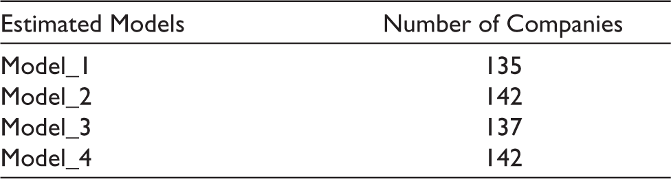
After selecting the companies, box plots are used to detect the outliers in the data because regression analysis is very sensitive to outliers. Hence, to produce the more accurate and reliable results the outliers are removed from the data. In the present study, an attempt is made to examine the power of Altman’s Z-score up to three years prior to the year for which returns are used as dependent variable and four different models are estimated by using simple linear regression. Thus, it is obvious that the outliers may vary from one model to another as the independent variables change across these models. As a result, after removing the outliers from the data the number of companies used to estimate these models vary from one model to another, and minimum and maximum number of companies used for this are 135 and 142, respectively. The number of companies used to estimate four different models are presented in Table 1.

Table 1.

Number of Observations Used to Estimate the Regression Models

Estimated Models	Number of Companies
Model_1	135
Model_2	142
Model_3	137
Model_4	142

Source: Authors’ calculation.

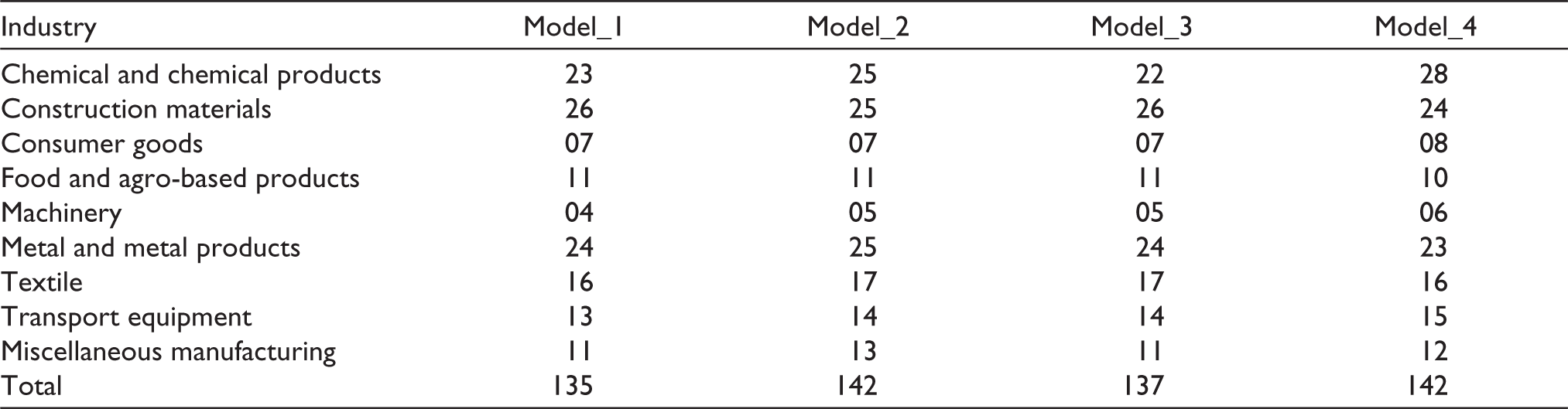
The selected companies are from different industries, which are chemicals and chemical products, construction materials, consumer goods, foods and agro-based products, machinery metals and metal products, miscellaneous manufacturing, textiles and transport equipment (see Table 2).

Table 2.

Industry Classification of Sample Companies

Industry	Model_1	Model_2	Model_3	Model_4
Chemical and chemical products	23	25	22	28
Construction materials	26	25	26	24
Consumer goods	07	07	07	08
Food and agro-based products	11	11	11	10
Machinery	04	05	05	06
Metal and metal products	24	25	24	23
Textile	16	17	17	16
Transport equipment	13	14	14	15
Miscellaneous manufacturing	11	13	11	12
Total	135	142	137	142

Source: Authors’ calculation.

Variables Used: Dependent and Independent

In the present study, Altman’s model is used as a measure of default risk to examine the relationship between default risk and stock returns by applying simple linear regression. Description of dependent and independent variables used to run the regression analysis is as follows:

Dependent Variable

The purpose of the study is to examine the relationship between default risk and stock returns, that is, whether stock returns are increasing or decreasing function of default risk. Hence, stock returns are used as a dependent variable to estimate the four regression models. The change in the adjusted closing prices (capital gain or loss) is used to calculate the stock returns as used by Tandiontong and Sitompul (2017). Stock returns are calculated as:

R_{S} = (P_{1} - P_{0}) / P_{0} \times 100

where

R_S = Stock return for the year

P₁ = Adjusted closing price for the current year

P₀ = Adjusted closing price for the previous year

Stock return for the year 2019 (R₂₀₁₉) is considered as a dependent variable to run the regression analysis.

Independent Variable

Altman’s model (1968) is used as a measure of default risk in the present study. Altman’s model is based on five ratios used as variables in the model and after multiplying these ratios with their coefficients, the overall score produced by the Altman’s model is known as Altman’s Z-score. Altman’s Z-score is calculated as below:

Z = 1.2 \times X_{1} + 1.4 \times X_{2} + 3.3 \times X_{3} + 0.6 \times X_{4} + 0.99 \times X_{5}

where

Z = Altman’s Z-score

X₁ = working capital / total assets

X₂ = retained earnings / total assets

X₃ = earnings before interest and tax / total assets

X₄ = market value of equity / total liabilities

X₅ = sales / total assets

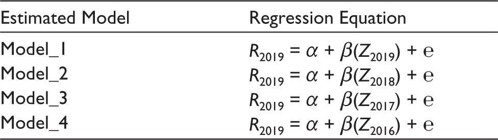
The Z-score produced by the model is used as independent variable to run the regression analysis. Altman (1968) claimed that Z-score can be used to predict the probability of default up to two years prior to the year of default. Hence, besides considering the current year’s Z-score as independent variable to predict the stock returns, earlier year’s Z-scores are also taken as independent variable in different regression models, respectively, to examine their predictive accuracy of future stock returns. The estimations of different regression models are presented in Table 3.

where

R₂₀₁₉ = Stock return calculated for the year 2019

Z₂₀₁₉ = Z-score calculated for the year 2019

Z₂₀₁₈ = Z-score calculated for the year 2018

Z₂₀₁₇ = Z-score calculated for the year 2017

Z₂₀₁₆ = Z-score calculated for the year 2016

Table 3.

Dependent and Independent Variables Used to Estimate Regression Models

Estimated Model	Regression Equation
Model_1	R₂₀₁₉ = α + β(Z₂₀₁₉) + ℮
Model_2	R₂₀₁₉ = α + β(Z₂₀₁₈) + ℮
Model_3	R₂₀₁₉ = α + β(Z₂₀₁₇) + ℮
Model_4	R₂₀₁₉ = α + β(Z₂₀₁₆) + ℮

Source: Authors’ calculation.

Results and Discussions

Descriptive Statistics

Descriptive statistic presents the data in summary form in order to describe the basic features of the data. The descriptive statistics of the variable is shown in Table 4.

Table 4.

Descriptive Statistics of Variables

Model_1
Variables	Observations	Mean	Standard Deviation	Minimum	Maximum
R ₂₀₁₉	135	−21.36896	24.48891	−76.5	49.08
Z ₂₀₁₉	135	2.073111	1.532847	−2	5.54
Model_2
Variables	Observations	Mean	Standard Deviation	Minimum	Maximum
R ₂₀₁₉	142	−20.39	25.97825	−83.07	53.83
Z ₂₀₁₈	142	2.398592	1.867046	−2.33	7.05
Model_3
Variables	Observations	Mean	Standard Deviation	Minimum	Maximum
R ₂₀₁₉	137	−21.70226	23.80131	−83.07	38.31
Z ₂₀₁₇	137	2.165182	1.578331	−1.61	5.93
Model_4
Variables	Observations	Mean	Standard Deviation	Minimum	Maximum
R ₂₀₁₉	142	−18.7912	26.12984	−83.07	58.06
Z ₂₀₁₆	142	1.893099	1.458719	−2.06	4.93

Source: Authors’ calculation.

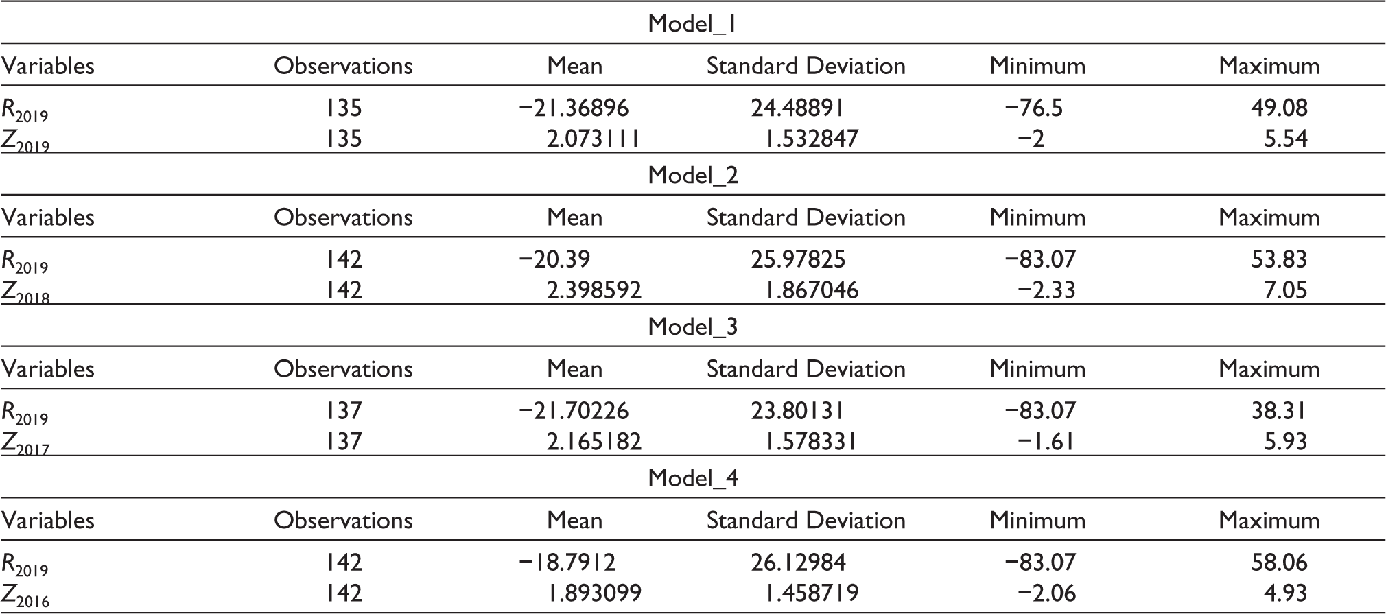
Descriptive statistics shows that the average values of returns for Model_1, Model_2, Model_3 and Model_4 are found to be negative having a moderate level of dispersion from the mean as measured by the standard deviation. Minimum figures of return indicate that the return is found to be negative in some cases and maximum figure of return indicates that some companies earned decent returns. The average value of Z-score is found to be positive for Model_1, Model_2, Model_3 and Model_4, respectively. Minimum value of Z-score is found to be negative, which indicates that some companies have negative value of Altman’s Z-score and others have positive value of Altman’s Z-score.

Correlation Analysis

Correlation analysis is a statistical method that measures the strength of relationship between two or more variables. A high correlation between two variables indicates that they are strongly related to each other and the lower correlation indicates a weak or no relationship between the two variables.

To analyse the strength of relationship between the dependent variable (R₂₀₁₉) and independent variables, that is, Z₂₀₁₉, Z₂₀₁₈, Z₂₀₁₇ and Z₂₀₁₆, respectively, simple correlation analysis is applied (see Table 5).

Table 5.

Results of Correlation Analysis (Pearson’s Correlation)

Model_1
	R ₂₀₁₉	Z ₂₀₁₉
R ₂₀₁₉	1	0.3479^***
Z ₂₀₁₉	0.3479^***	1
Model_2
	R ₂₀₁₉	Z₂₀₁₈
R ₂₀₁₉	1	0.1755^**
Z ₂₀₁₈	0.1755^**	1
Model_3
	R ₂₀₁₉	Z₂₀₁₇
R ₂₀₁₉	1	0.1757^**
Z ₂₀₁₇	0.1757^**	1
Model_4
	R ₂₀₁₉	Z₂₀₁₆
R₂₀₁₉	1	0.1380
Z₂₀₁₆	0.1380	1

Source: Authors’ calculation.

Notes: ^***Significant at 1%.

^**Significant at 5%.

Results of the Pearson correlation method indicate that there is positive association between Altman’s Z-score and return. This relationship indicates that increase in Z-score results into the increase in the returns. Altman’s Z-score for the same year (Z₂₀₁₉), one year prior Z-score (Z₂₀₁₈) and two years prior Z-score (Z₂₀₁₇) are found to be significantly associated with the returns in the year 2019 (R₂₀₁₉) and three years prior Z-score (Z₂₀₁₆) is found to be insignificant which indicates that three years prior Z-score (Z₂₀₁₆) is not associated with the returns in the year 2019 (R₂₀₁₉).

The Pearson correlation of the same year’s Z-score (Z₂₀₁₉) and returns in the year 2019 is found to be 0.3479, which decreases when calculated for one year prior Z-score (Z₂₀₁₈), two years prior Z-score (Z₂₀₁₇), which indicates that same year Z-score is more closely associated with the stock returns.

Regression Analysis

Regression analysis is the statistical analysis used to understand the relationship among the variables and to predict the variable of interest based on the other variables. The variable of interest is known as dependent variable or outcome variable and the variables used to predict the dependent variable are known as independent variables or explanatory variables. Linear regression is the study of linear relationship between variables and is a widely used technique. Linear regression estimates the regression line to predict the dependent variable that can be written as:

Y = α + β_{1} X_{1} + β_{2} X_{2} + \dots + β_{n} X_{n} + e

where

Y = dependent variable

α = constant or intercept

β₁, β_2, β_n = slopes of the regression line

℮ = error term

The regression equation assumes that dependent variable (Y) is a straight-line function of independent variables (X₁, X_2, X₃) holding other things constant. Constant or intercept (α) indicates the prediction made by the model if all the independent variables are found to be zero. Slopes of regression line (β) also known as beta coefficients that measures the change in dependent variable (Y) due to one unit change in independent variables (X₁, X_2, X₃), other things being equal. Error term (℮) indicates the prediction errors of the model, which is assumed to be independent and normally distributed. Linear regression is based on certain assumption, which must be satisfied in order to make the result more accurate and reliable because the violation of any of these assumptions leads to biased results.

Testing the Assumptions of Regression Analysis

There are some basic assumptions that must be satisfied to run the linear regression analysis. These assumptions are very critical because violation of these assumptions raise the question on the validity of the results. Hence, if all the assumptions are found to be satisfied then the results of regression analysis are considered to be reliable and robust enough. Following are the basic assumptions that are needed to be fulfilled are tested in the study:

Normality

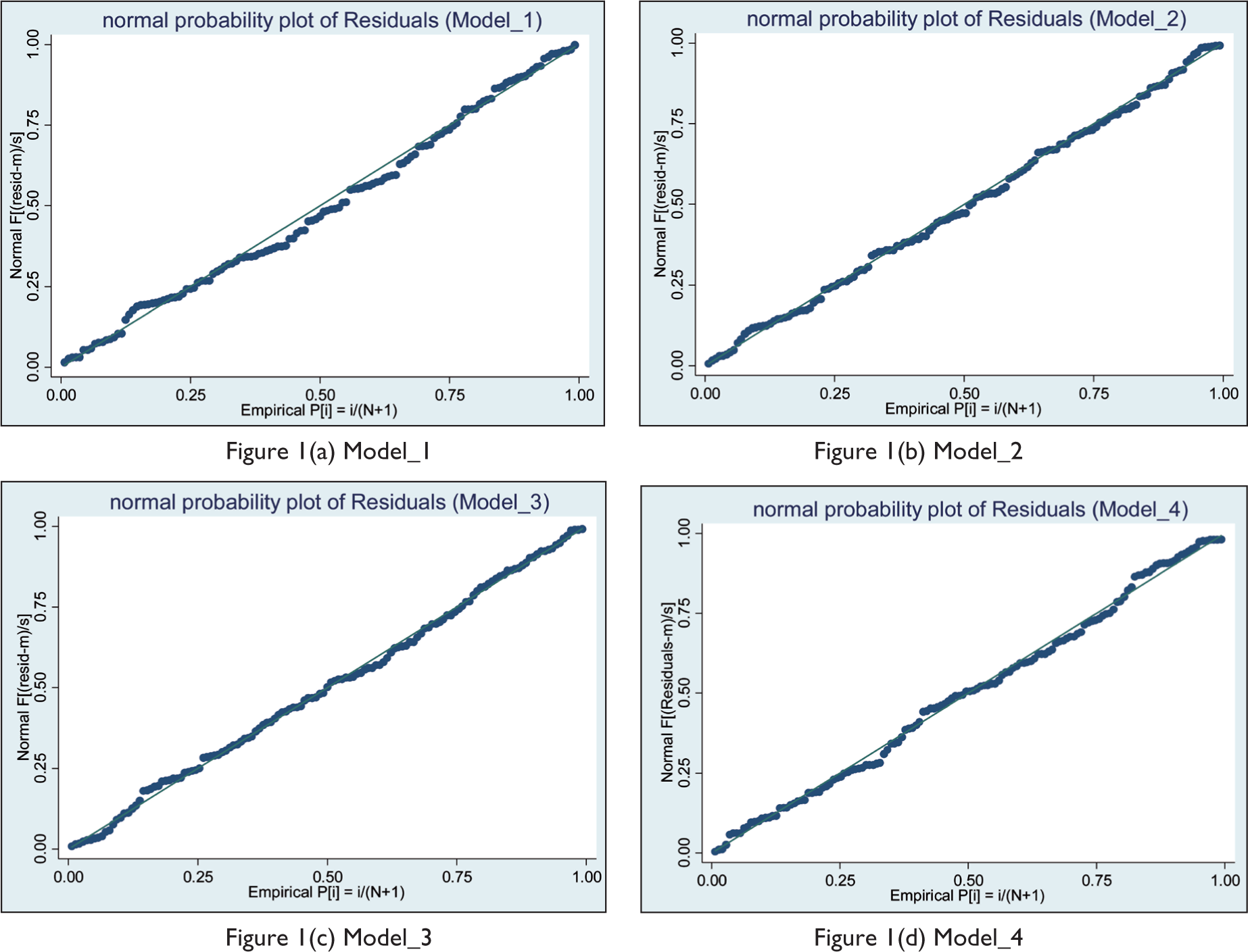
Normality is the mandatory condition to be satisfied to run the regression analysis. The violation of the normality assumption leads to the biased coefficients of the model that raise the question on the accuracy and reliability of the results. In the present study, normal P–P plot, Shapiro–Wilk test and skewness and kurtosis test for normality are used to assess the normality of the variables.

The normal probability plot is the graphical technique to check whether the data are normally distributed or not. If the points form an approximate straight line then it is considered that data follow the assumption of normal distribution. As shown in Figure 1 the normal probability plots for Model_1, Model_2, Model 3 and Model_4 exhibit the formation of straight line, hence it can be concluded that data are normally distributed. Apart from graphical method, two tests namely Shapiro–Wilk test and skewness and kurtosis test for normality are also performed to ensure the normality of the data and the results of both tests are presented in Tables 6 and 7, respectively.

Figure 1.

Source: Based on authors’ analysis.

Table 6.

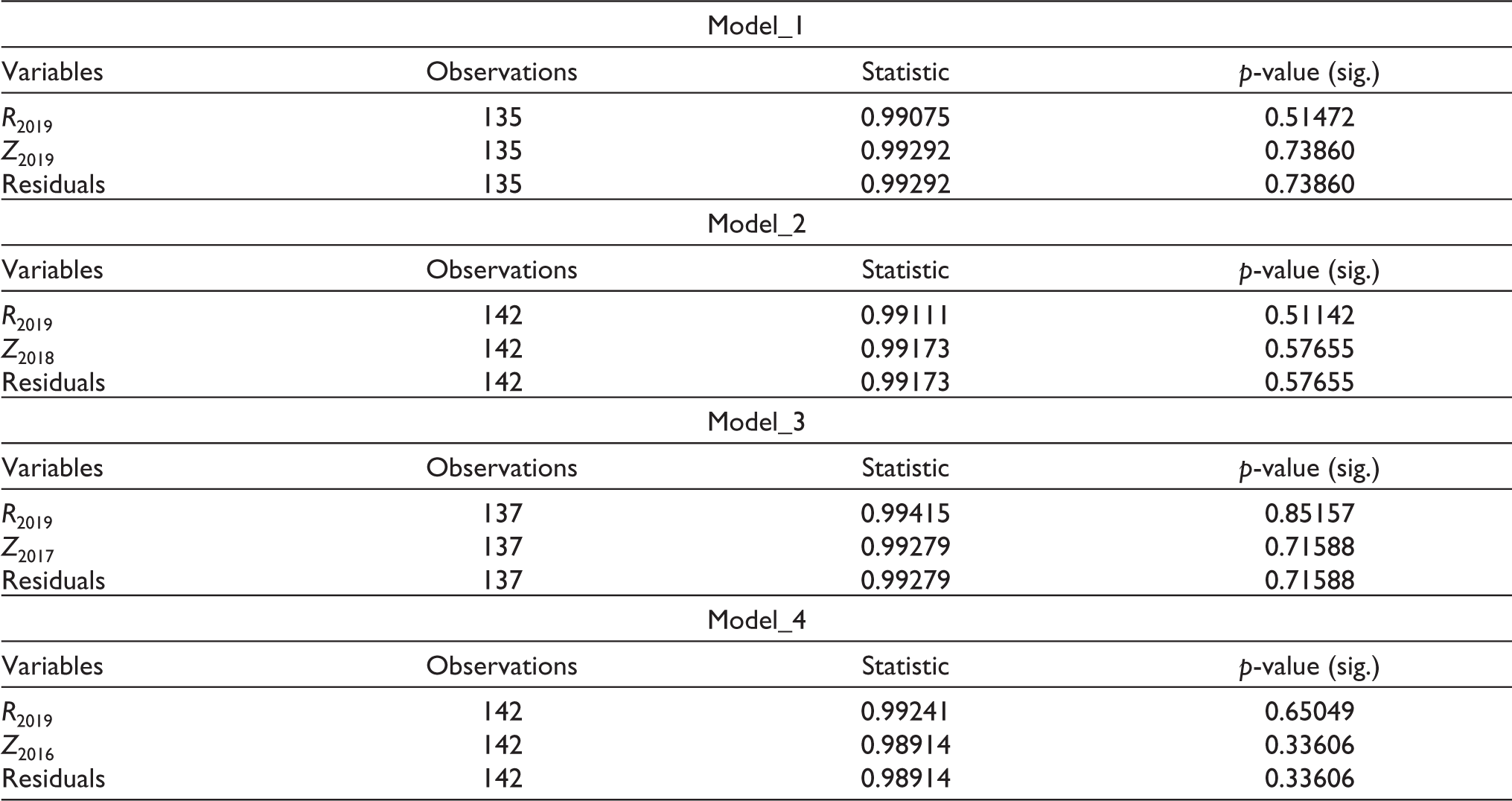
Results of Shapiro–Wilk Test

Model_1
Variables	Observations	Statistic	p-value (sig.)
R ₂₀₁₉	135	0.99075	0.51472
Z ₂₀₁₉	135	0.99292	0.73860
Residuals	135	0.99292	0.73860
Model_2
Variables	Observations	Statistic	p-value (sig.)
R ₂₀₁₉	142	0.99111	0.51142
Z ₂₀₁₈	142	0.99173	0.57655
Residuals	142	0.99173	0.57655
Model_3
Variables	Observations	Statistic	p-value (sig.)
R ₂₀₁₉	137	0.99415	0.85157
Z ₂₀₁₇	137	0.99279	0.71588
Residuals	137	0.99279	0.71588
Model_4
Variables	Observations	Statistic	p-value (sig.)
R ₂₀₁₉	142	0.99241	0.65049
Z ₂₀₁₆	142	0.98914	0.33606
Residuals	142	0.98914	0.33606

Source: Authors’ calculation.

Note: p > 0.05 indicates that data are normally distributed.

Table 7.

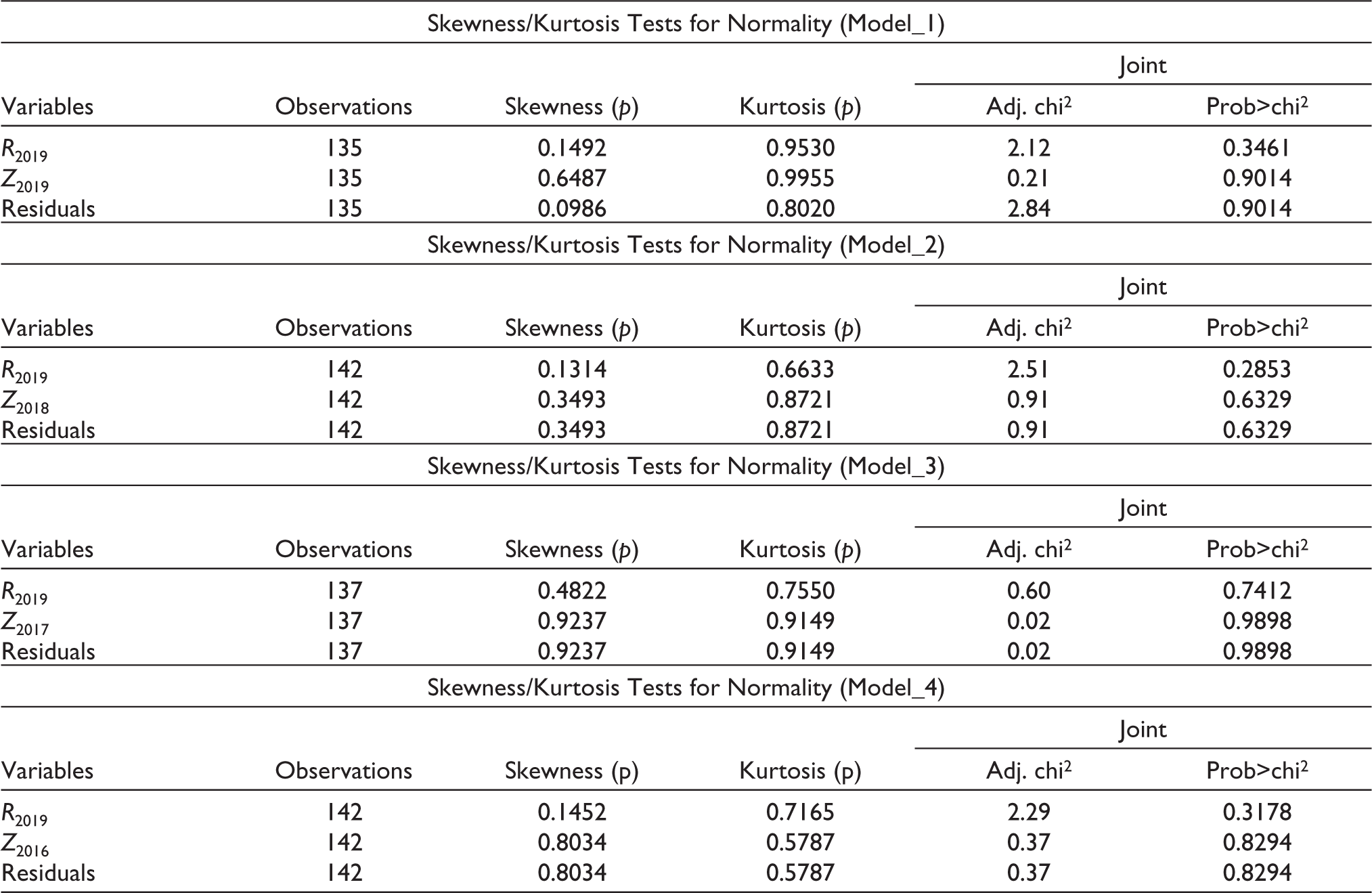
Results of Skewness/Kurtosis Tests

Skewness/Kurtosis Tests for Normality (Model_1)
Variables	Observations	Skewness (p)	Kurtosis (p)	Joint
Variables	Observations	Skewness (p)	Kurtosis (p)	Adj. chi²	Prob>chi²
R ₂₀₁₉	135	0.1492	0.9530	2.12	0.3461
Z ₂₀₁₉	135	0.6487	0.9955	0.21	0.9014
Residuals	135	0.0986	0.8020	2.84	0.9014
Skewness/Kurtosis Tests for Normality (Model_2)
Variables	Observations	Skewness (p)	Kurtosis (p)	Joint
Variables	Observations	Skewness (p)	Kurtosis (p)	Adj. chi²	Prob>chi²
R ₂₀₁₉	142	0.1314	0.6633	2.51	0.2853
Z ₂₀₁₈	142	0.3493	0.8721	0.91	0.6329
Residuals	142	0.3493	0.8721	0.91	0.6329
Skewness/Kurtosis Tests for Normality (Model_3)
Variables	Observations	Skewness (p)	Kurtosis (p)	Joint
Variables	Observations	Skewness (p)	Kurtosis (p)	Adj. chi²	Prob>chi²
R ₂₀₁₉	137	0.4822	0.7550	0.60	0.7412
Z ₂₀₁₇	137	0.9237	0.9149	0.02	0.9898
Residuals	137	0.9237	0.9149	0.02	0.9898
Skewness/Kurtosis Tests for Normality (Model_4)
Variables	Observations	Skewness (p)	Kurtosis (p)	Joint
Variables	Observations	Skewness (p)	Kurtosis (p)	Adj. chi²	Prob>chi²
R ₂₀₁₉	142	0.1452	0.7165	2.29	0.3178
Z ₂₀₁₆	142	0.8034	0.5787	0.37	0.8294
Residuals	142	0.8034	0.5787	0.37	0.8294

Source: Authors’ calculation.

Note: p > 0.05 indicates that data are normally distributed.

Results of the Shapiro–Wilk test indicate that if the p-values are greater than 0.05 indicates null hypothesis, that is, data that are normally distributed are accepted. Hence, on the basis of the results of Shapiro–Wilk test, it is evidenced that data are normally distributed. Another test of normality namely skewness/kurtosis tests for normality is also used to determine whether data are normally distributed or not.

Results of skewness/kurtosis tests for normality indicates that the null hypothesis, that is, data are normally distributed is accepted as the p-values of the test are found to be greater than 0.05 for all the variables in case of Model_1, Model_2, Model_3 and Model_4. Hence, it is evidenced from the results of Shapiro–Wilk test and skewness/kurtosis tests for normality that the assumption of normality is not violated and the data are normally distributed.

Linearity

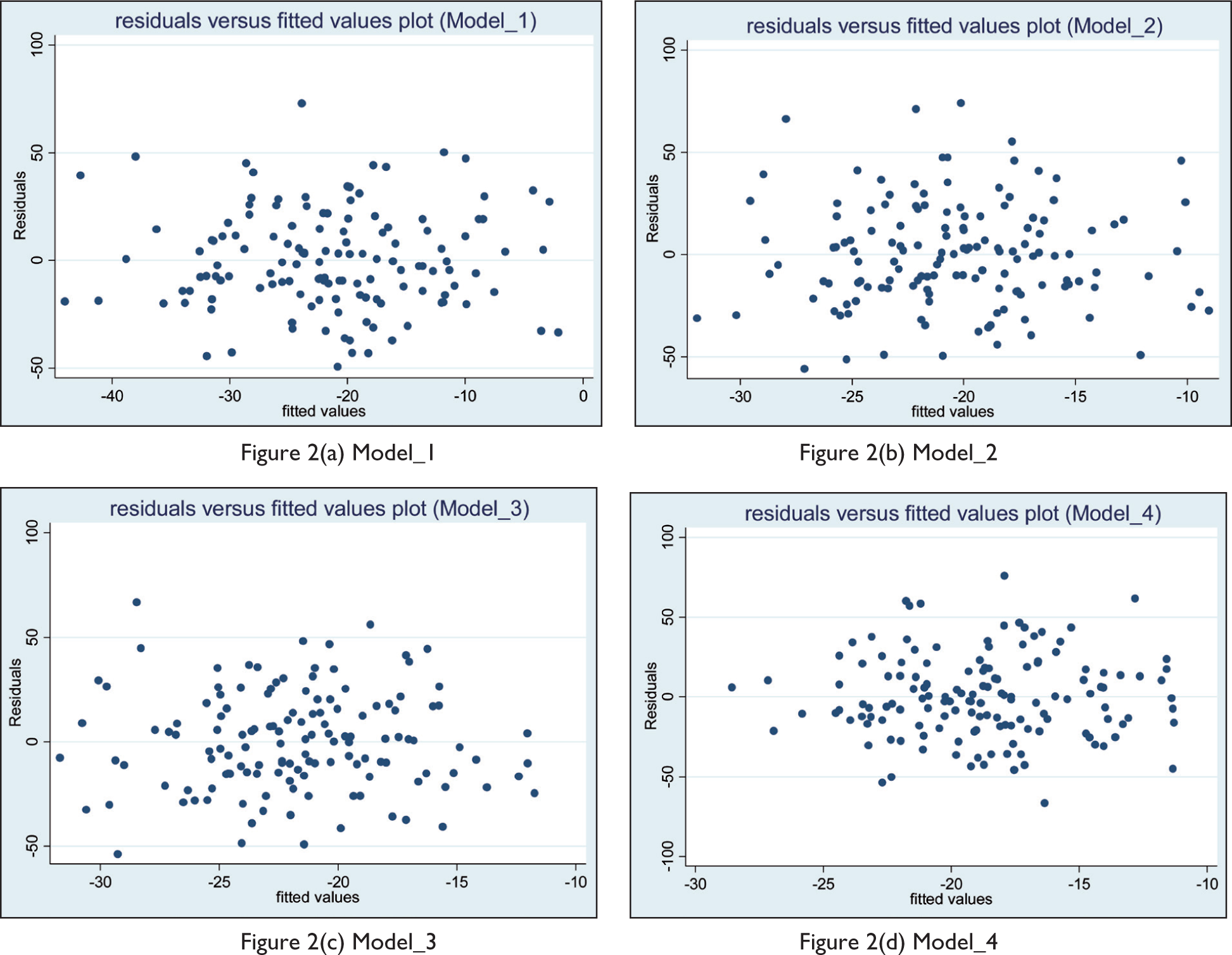
The assumption of linearity indicates the linear relationship between the independent variable and dependent variable. In other words, the assumption of linear relationship indicates that one unit change in independent variable results into the change in the dependent variable and this change in dependent variable is constant. This assumption of linear relationship between dependent variable and independent variable can be tested by using the scatter plots of residuals versus fitted values because if the residuals are found to be normally distributed and are homoscedastic then it is assumed that there is a linear relationship between the variables.

The residuals of Model_1, Model_2, Model 3 and Model_4 are found to be equally distributed which shows that data are homoscedastic and are normally distributed (see Figure 2). Hence, there is no problem of non-linearity and the variables are expected to have linear relationship.

Absence of Multicollinearity

Multicollinearity is related to the presence of linear relationship among independent variables. Regression analysis assumes no multicollinearity among the independent variables in order to run the analysis because it becomes difficult to exhibit the true relationship of independent variables with the dependent variable in the presence of multicollinearity. Multicollinearity condition occurs when the independent variables are found to be moderately or highly correlated. Correlation analysis or variance inflation factor (VIF) can be used to assess whether the problem of multicollinearity is present among the variables or not. In the present study only one variable Altman’s Z-score is used as independent variable, hence the assumption of multicollinearity becomes irrelevant to test and hence, there was no need to check the assumption of multicollinearity.

Homoscedasticity

The assumption of homoscedasticity is related to the constant variance in the error term or residuals. If the variance in the error term or residuals is not found to be constant, it is known as the problem of heteroscedasticity. The main reason for the presence of the non-constant variance in the error term or residuals is the presence of outliers in the data. The problem of heteroscedasticity or the assumption of constant variance in the error term can be tested through residual versus fitted values plot, Breusch–Pagan/Cook–Weisberg test for heteroscedasticity and White’s test for homoscedasticity. In the present study, all three are used to test the assumption of homoscedasticity.

The residuals of Model_1, Model_2, Model_3 and Model_4 are found to be equally distributed which shows that data are homoscedastic and there is no problem of heteroscedicity (see Figure 2). Apart from the residuals versus fitted values plot, two tests namely Breusch–Pagan/Cook–Weisberg test for heteroscedasticity and White’s test for homoscedasticity are also used to test the assumption of homoscedasticity.

Figure 2.

Source: Based on authors’ analysis.

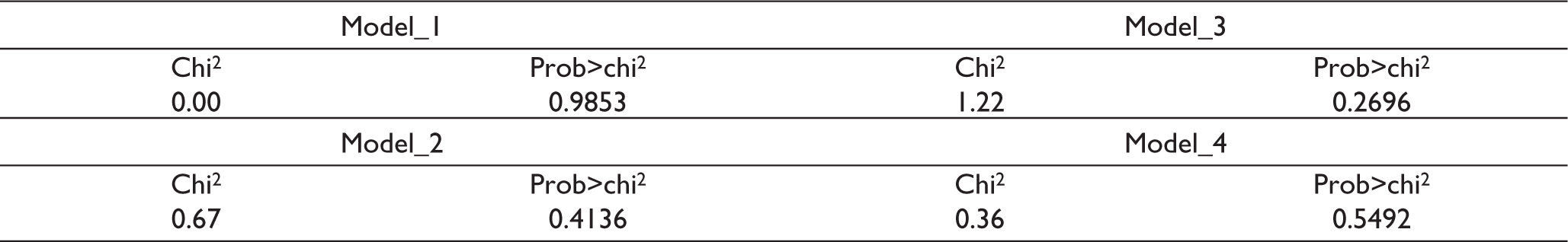
Results of Breusch–Pagan / Cook–Weisberg test for heteroscedasticity indicate that the null hypothesis of constant variance is accepted as the p-values of the test are found to be greater than 0.05 in case of Model_1, Model_2, Model_3 and Model_4 (see Table 8). Thus, it can be concluded that there is no problem of heteroscedasticity and there is a constant variance in the error term. Another test named as White’s test for homoscedasticity is also used to check the assumption of homoscedasticity.

Table 8.

Results of Breusch–Pagan / Cook–Weisberg Test

Model_1		Model_3
Chi²	Prob>chi²	Chi²	Prob>chi²
0.00	0.9853	1.22	0.2696
Model_2		Model_4
Chi²	Prob>chi²	Chi²	Prob>chi²
0.67	0.4136	0.36	0.5492

Source: Authors’ calculation.

Note: p > 0.05 indicates that there is no problem of heteroscedasticity.

Results of White’s test for homoscedasticity indicate that the null hypothesis of homoscedasticity is accepted as the p-values of the test are found to be greater than 0.05 in case of Model_1, Model_2, Model_3 and Model_4 (see Table 9). Thus, it can be concluded that there is no problem of heteroscedasticity and there is a constant variance in the error term. Thus, the results of both the test proved that there is a constant variance in the error term and there is no problem of heteroscedasticity.

Table 9.

Results of White’s Test

Model_1		Model_3
Chi²	Prob>chi²	Chi²	Prob>chi²
0.22	0.8945	1.94	0.3790
Model_2		Model_4
Chi²	Prob>chi²	Chi²	Prob>chi²
1.24	0.5382	1.96	0.3750

Source: Authors’ calculation.

Note: p > 0.05 indicates that there is no problem of heteroscedasticity.

No Autocorrelation

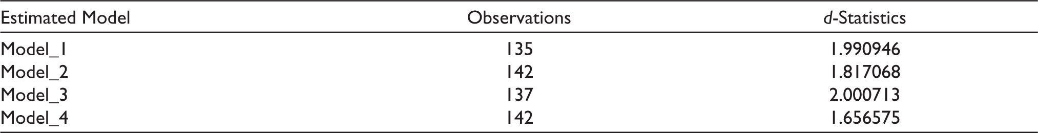
Autocorrelation causes problem in the linear regression analysis, hence, should be corrected before running the linear regression analysis. Durbin–Watson test and Breusch–Godfrey/LM test for autocorrelation are used to check the assumption of autocorrelation. The values given by Durbin–Watson test lies between 0 and 4. A value of 2 means there is no problem of autocorrelation; however, the rule of thumb is that the value between 1.5 and 2.5 is relatively normal, but the values below 1.5 and above 2.5 cause the serious problem of autocorrelation.

The values for the Durbin–Watson test for Model_1 and Model_2 are found to be nearest to the value of 2 and the value for Model_3 is almost equal to the value of 2. The value of Durbin–Watson test for Model_4 is 1.656575 which is little bit far from the value of 2, but it is within the range of 1.5–2.5. Hence, it can be concluded on the basis of the results of Durbin–Watson test that there is no serious problem of autocorrelation in the data (see Table 10).

Table 10.

Results of Durbin–Watson Test

Estimated Model	Observations	d-Statistics
Model_1	135	1.990946
Model_2	142	1.817068
Model_3	137	2.000713
Model_4	142	1.656575

Source: Authors’ calculation.

Note: 1.5 < d-statistics > 2.5 indicates there is no problem of autocorrelation.

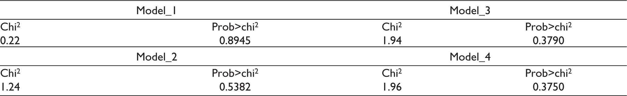
To further validate the assumption of autocorrelation another test named as Breusch–Godfrey/ LM test for autocorrelation is performed. Results of Breusch–Godfrey/ LM test for autocorrelation indicates a null hypothesis, that is, no serial correlation is accepted as the p-values of the test are found to be greater than 0.05 in case of Model_1, Model_2, Model_3 and Model_4 (see Table 11). Thus, it can be concluded that there is no problem of autocorrelation. The results of both the tests proved that there is no problem of autocorrelation or serial correlation.

Table 11.

Results of Breusch–Godfrey/LM Test

Model_1		Model_3
Chi²	Prob>chi²	Chi²	Prob>chi²
0.000	0.9826	0.053	0.8171
Model_2		Model_4
Chi²	Prob>chi²	Chi²	Prob>chi²
0.789	0.3745	3.102	0.0782

Source: Authors’ calculation.

Note: p > 0.05 indicates that there is no problem of autocorrelation.

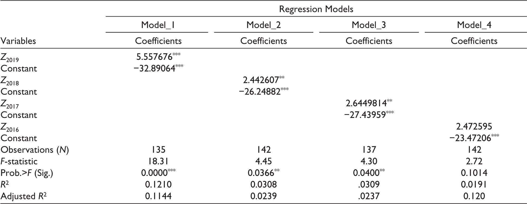
After checking that all the basic assumptions are satisfied and none of these assumptions is violated, the simple linear regression analysis is performed. To run the regression analysis, returns of companies in the year 2019 are used as dependent variable (R₂₀₁₉) and Altman’s Z-score in the years 2019, 2018, 2017 and 2016 is used as independent variable (Z₂₀₁₉, Z₂₀₁₈, Z₂₀₁₇, Z₂₀₁₆) to examine the explanatory power of Altman’s Z-score as a measure of default risk. The results of regression analysis are presented in Table 12.

Table 12.

Results of Regression Analysis

Variables	Regression Models
	Model_1	Model_2	Model_3	Model_4
	Coefficients	Coefficients	Coefficients	Coefficients
Z ₂₀₁₉	5.557676^***
Constant	−32.89064^***
Z ₂₀₁₈		2.442607^**
Constant		−26.24882^***
Z ₂₀₁₇			2.6449814^**
Constant			−27.43959^***
Z ₂₀₁₆				2.472595
Constant				−23.47206^***
Observations (N)	135	142	137	142
F-statistic	18.31	4.45	4.30	2.72
Prob.>F (Sig.)	0.0000^***	0.0366^**	0.0400^**	0.1014
R ²	0.1210	0.0308	.0309	0.0191
Adjusted R²	0.1144	0.0239	.0237	0.120

Source: Authors’ calculation.

Notes: ^***Significant at 1%.

^**Significant at 5%.

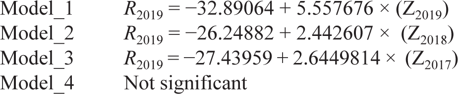
Results of regression analysis indicate that Altman’s Z-score is found to be significant in Model_1, Model_2 and Model_3 whereas it is found to be insignificant in case of Model_4. These results indicate that one year prior and two years prior Altman’s Z-score can be used as an explanatory variable to returns. Secondly, the beta coefficient of Altman’s Z-score is found to be positive, which indicates the positive relationship between Altman’s Z-score and returns. It means increase in Z-score leads to increase in returns earned by the company. In the present study, Altman’s Z-score is used as a measure of the default risk. Higher the Z-score value indicates that company is financially strong and there are no or less chances of default. On the other hand, lower value of Altman’s Z-score indicates that a company is in distress zone and the likelihood of default is very high. It indicates that higher the Altman’s Z-score lower will be the chances of default and hence, Altman’s Z-score is negatively associated with default risk. As the regression results presented in Table 12 indicates that Altman’s Z-score is positively related to returns, thus indicating that higher the Z-score, the higher will be the returns. It can be concluded that higher Altman’s Z-score lower will be the default risk and higher will be the returns. This relationship indicates that default risk is negatively related with the returns. Similar findings were reported by Dichev (1998) and Campbell et al. (2011) by concluding that distress risk is unsystematic and there is negative relationship between default risk and stock returns. This negative relationship between default risk and stock returns evidenced the market inefficiency (Chava & Purnanandam, 2010). Zhao (2015) also reported that the Z-score and returns are positively related which indicate that higher the Z-score higher will be the returns. In other words, higher the Z-score lower will be the default risk and higher will be the returns and hence, default risk is negatively related to stock returns. The beta coefficients presented in the Table 12 can be used to predict the returns and regression equation for the models can be written as:

\begin{array}{l} Model_1 R_{2019} = - 32.89064 + 5.557676 \times (Z_{2019}) \\ Model_2 R_{2019} = - 26.24882 + 2.442607 \times (Z_{2018}) \\ Model_3 R_{2019} = - 27.43959 + 2.6449814 \times (Z_{2017}) \\ Model_4     Not significant \end{array}

The F-statistic for Model_1, Model_2 and Model_3 is found to be significant which indicates that the regression models are statistically significant to predict the dependent variable. Hence, on the basis of these results it is found that up to two years prior Z-score can be used to predict the returns. The F-statistic for Model_4 is found to be insignificant which indicates that three years prior Z-score is not able to predict the return. The R-square (R²) value indicates the variation in the dependent variable explained by the model. The R² value for Model_1, Model_2, Model_3 and Model_4 are found to be 0.1210, 0.0308, 0.0309 and 0.0191, respectively. These values indicate that the Model_1, Model_2, Model_3 and Model_4 explained the 12.10%, 3.08%, 3.09% and 1.91% variation in the returns, respectively. These results indicate that Model_1 is the best model as it explained highest variation in the return and Model_4 is worst model and found to be insignificant too. Model_2 and Model_3 explained almost similar percentage of variation in the stock return. Adjusted R² is the modified version of R² which is adjusted for number of variables as predictors in the model. Adjusted R² only increases if the new added variable improves the model. Hence, on the basis of R² and Adjusted R² values Model_1 is found to be significant and is proved to be the best model to predict the returns. It is concluded that one and two years prior Altman’s Z-score can be used as predictor of returns but the same year Z-score predicts the returns better than one year and two years prior Z-score. Altman’s Z-score can be used as a measure of default risk and the result indicates that higher the Z-score lower will be the default risk and higher will be the returns; hence, default risk is negatively associated with returns.

Conclusions

To examine the relationship between default risk and stock return, Altman’s model (1968) is used as a measure of default risk. Altman’s model is based on five ratios used as variables in the model and after multiplying these ratios with their coefficients, the overall score produced by Altman’s model is known as Altman’s Z-score. This Z-score is used as a measure of default risk and used to examine the relationship between default risk and stock returns. The Z-score values up to three years prior to the year for which returns are taken as dependent variable are also taken along with the same year Z-score in order to examine the predictive accuracy of the Z-score to predict the stock returns. Four different models are estimated by using simple linear regression analysis. Before running the regression analysis outliers are removed from the data and all the basic assumptions are tested. Results indicate that all the assumptions are satisfied. The results of correlation analysis indicate that there is positive association between Altman’s Z-score and return. This relationship indicates that increase in Z-score results into the increase in the stock returns. Altman’s Z-score for the same year (Z₂₀₁₉), one year prior Z-score (Z₂₀₁₈) and two years prior Z-score (Z₂₀₁₇) are found to be significantly associated with the returns in the 2019 (R₂₀₁₉) and three years prior Z-score (Z₂₀₁₆) is found to be insignificant which indicates that three years prior Z-score (Z₂₀₁₆) is not associated with returns in the year 2019 (R2₀₁₉). The Pearson correlation of same year Z-score (Z₂₀₁₉) and stock returns is found to be 0.3479, which decreases when calculated for one year prior Z-score (Z₂₀₁₈), two years prior Z-score (Z₂₀₁₇) with stock returns in the year 2019 (R₂₀₁₉). It indicates that same year Z-score is more associated with stock returns. Results of regression analysis indicate that Altman’s Z-score is found to be significant in Model_1, Model_2 and Model_3, whereas it is found to be insignificant in case of Model_4. The F-statistic for Model_1, Model_2 and Model_3 is found to be significant, which indicates that the regression models are statistically significant in predicting the dependent variable. These results indicate that same year, one year prior and two years prior Altman’s Z-score can be used as explanatory variable to returns. The F-statistic for Model_4 is found to be insignificant, which indicates that four years prior Z-score is not able to predict the stock return. R² values indicate that Model_1 is the best model as it has explained highest variation (12.10%) in the stock return and Model_4 is worst model that explained lowest variation in stock return (1.91%) in comparison to other models. Model_2 and Model_3 explained almost similar percentage of variation in the stock return, that is, 3.08% and 3.09%, respectively. The beta coefficient of Altman’s Z-score is found to be positive, which indicates the positive relationship between Altman’s Z-score and stock returns. It means increase in Z-score leads to increase in stock returns. It can be concluded that higher the Altman’s Z-score, lower will be the default risk and higher will be the returns. This relationship indicates that default risk is negatively related with the stock returns. Similar findings are reported by Dichev (1998) and Campbell et al. (2011) by concluding that distress risk is unsystematic and there is negative relationship between default risk and stock returns. Zhao (2015) also reported that the Z-score and returns are positively related, which indicate that higher the Z-score, higher will be the returns. In nutshell, Altman’s Z-score can be used as a measure of default risk, and results indicate the existence of positive relationship between Z-score and stock return and hence a negative relationship between default risk and stock return.

The findings of the study have practical implications for the different sections of society. Primarily the study findings will be of immense use to the stock market analysts, equity researchers and investors. The study observed that there exists negative relationship between default risk and stock returns and therefore the investors should invest in the companies having higher Z-score to get higher returns as these companies are less prone to default risk The study findings suggest that the default risk is an unsystematic risk as the market do not reward investors for bearing higher default risk. Thus, it becomes imperative for investors to design their portfolios in a manner that the default risk is well diversified. Furthermore, the study findings also suggest that the investors may use default risk as measured by Altman’s Z-score to predict both the short-run and the long-run equity returns. Secondly, the findings of the research will also be useful for the banking sector in taking their lending decisions. Since the findings of the research shows the existence of negative relationship between default risk and stock returns thus indicating that the high default risk companies may observe deterioration in their market capitalization in the near future. Such decrease in future market capitalization of companies will further worsen the debt equity ratio of the company and thus will add further to the default risk of the company and thus making it difficult for the company to raise additional finance. Thus, while approving loans to companies having poor Z-score the banks should also consider the potential fall in the market capitalization of such companies in the near future.

The present research only considered default risk as measured by Altman’s model for predicting future stock returns. However, there exists other models too that can be used as a measure of default risk. Hence, further research in this area using other models as a measure of default risk can be conducted to validate the results of this study and to strengthen the evidence on the unsystematic nature of the default risk.

Footnotes

Declaration of Conflicting Interests

The authors declared no potential conflicts of interest with respect to the research, authorship and/or publication of this article.

Funding

The authors received no financial support for the research, authorship and/or publication of this article.

References

Afrin

(2017). Analysing the potential of Altman’s z-score for prediction of market performance and share return – A case study of the cement industry in Bangladesh. The AUST Journal of Science and Technology, 1(2), 1–16.

Altman

E. I.

(1968). Financial ratios, discriminant analysis and the prediction of corporate bankruptcy. The Journal of Finance, 23(4), 589–609.

Apergis

, Sorros

, Artikis

, & Zisis

(2011). Bankruptcy probability and stock prices: The effect of Altman’s z-score information on stock prices through panel data. Journal of Modern Accounting and Auditing, 7(7), 689–696.

Arbel

, Kolodny

, & Lakonishok

(1977). The relationship between risk of default and return on equity: an empirical investigation. The Journal of Financial Quantitative Analysis, 12(4), 615–625.

Avramov

, Chordia

, Jostova

, & Philipov

(2009). Credit ratings and the cross-sections of stock returns. Journal of Financial Markets, 12, 469–499.

Beaver

W. H.

(1966). Financial ratios as predictors of failure. Journal of Accounting Research, 4, 71–111.

Campbell

J. Y.

, Hilscher

J. D.

, Szilagyi

(2011). Predicting financial distress and performance of distress stocks. Journal of Investment Management, 9(2), 14–34.

Chava

, & Purnanandam

(2010). Is default risk negatively related to stock returns? The Review of Financial Studies, 23(6), 2523–2559.

Chen

, & Hill

(2013). The impact of diverse measures of default risk on UK stock returns. Journal of Banking and Finance, 37, 5118–5131.

10.

Czombera

(2014). Altman’s z-score: Credit ratings and equity investing in a high-quality environment. 1–45. https://www.academia.edu/8588487/Altman_Z-Score_Credit_Ratings_and_Equiy_Investing_in_a_High-Quality_Environment.

11.

Denis David

, & Denis

(1995). Causes of financial distress following leveraged re-capitalization. Journal of Financial Economics, 27, 411–418.

12.

Dichev

D. I.

(1998). Is the risk of bankruptcy a systematic risk? The Journal of Finance, 53(3), 1131–1147.

13.

Effendi

, Affandi

, & Sidharta

(2016). The effect of financial ratios based springate models to stock prices in telecommunication public companies. Journal of Economy, Business and Entrepreneurship, 10(1), 1–16.

14.

Ergut

(2015). Corporate default risk and stock returns: Evidence from the UK (Master’s Thesis, University of Amsterdam, Netherlands). http://www.scriptiesonline.uba.uva.nl/document/620865

15.

Fiordelisi

, & Marques

L. D.

(2013). Is bank default risk systematic? Journal of Banking and Finance, 37, 2000–2010.

16.

Garlappi

, Shu

, & Yan

(2008). Default risk, shareholder advantage and stock returns. Review of Financial Studies, 21(6), 2743–2778.

17.

Gharghori

, Chan

, & Faff

(2009). Default risk and equity returns. Pacific – Basin Finance Journal, 17, 580–593.

18.

Lang

L. H. P.

, & Stulz

(1992). Contagion and competitive intra-industry effect of bankruptcy announcements: An empirical analysis. Journal of Financial Economics, 8, 45–60.

19.

Lestari

D. S.

, Oktaviani

F. R.

, & Arafah

(2016). Financial distress prediction with Altman z-score and effect on stock prices: Empirical study on companies sub-sectors chemical listed in Indonesia Stock Exchange Period 2009-2014. International Journal of Business and Management Invention, 5(8), 30–39.

20.

Rietz

T. A.

(1988). The equity risk premium: A solution. Journal of Monetary Economics, 22, 117–131.

21.

Saji

T. G.

(2018). Financial distress and stock market failures: Lessons from Indian realty sector. Vision, 22(1), 1–11.

22.

Shumway

(2001). Forecasting bankruptcy more accurately: A simple hazard model. Journal of Business, 74, 101–124.

23.

Trandiontong

, & Sitompul

(2017). The influence of financial distress using Altman’s z-score, the beta of stocks and inflation to stock return. Journal of Finance and Banking Review, 2(2), 21–27.

24.

Vassalou

, & Xing

(2004). Default risk in equity returns. The Journal of Finance, 59(2), 831–868.

25.

Zhao

(2015). The Relationship between z-score and stock prices. Social Science Research Network, 1–36. https://dx-doi-org.web.bisu.edu.cn/10.2139/ssrn.2595600.