



Abstract
India has set an ambitious export target of US$0.5 trillion by 2025 and US$1 trillion by 2030 from US$291 billion in 2021 as part of its Atmanirbhar Bharat campaign. Since India opened up its economy in 1991, India has concluded several bilateral and regional free trade agreements. India signed a Comprehensive Economic Partnership Agreement (CEPA) with the United Arab Emirates in February 2022 and Economic Cooperation and Trade Agreement (ECTA) with Australia in April 2022. India is in the process of concluding trade agreements with the UK, the European Union, Canada, Israel and GCC countries. This article estimates the impact of all the above mentioned FTAs on India’s GDP and its components with an increased emphasis on its exports using a computable general equilibrium framework and machine learning techniques. The analysis estimates that the FTAs will boost India’s GDP by 4.10% to add US$109.096 billion in 2030 and the exports increase by 16.73% or US$46.08 billion. The exports from India to UAE, Australia, UK, European Union, Canada, Israel and GCC countries are estimated to increase by US$67.312 billion by 2030. This increase is relatively higher than the increase in aggregate exports of India suggesting a trade diversion from countries that are not part of the FTAs toward the seven countries with which India is anticipated to sign an FTA.
Introduction
The developmental gains to the economy from trade liberalization are well documented. The decades that followed the world wars called for multilateral cooperation between countries and the global trade landscape witnessed a surge in bilateral, multilateral and regional trade agreements. The average value of tariffs around the world has declined by 85% since 1947 following the efforts of the GATT and WTO (Kiyuti, 2018). Such liberalization efforts have expanded global trade which is evident from the rise in trade to GDP ratio from 25.01% in 1970 to 51.62% in 2020 (World Bank, 2022b).
According to WTO, there are various regional trade agreements in place covering 316 Free Trade Agreements, 186 Economic Integration Agreements and 18 Customs Union (WTO, 2022). These agreements have played a key role in shaping international trade evidenced by the fact that the promotion of global trade is key to the growth and development of the economy.
India has always envisioned regional and bilateral trade agreements as an essential tool to promote trade and investment and has effected several trade agreements and policy measures since it opened its economy in 1991. India has entered into 45 trade agreements including preferential agreements. Beyond offering preferential tariff rates in the trade happening between India and the countries that are parties to the agreement, it also fosters broader cooperation, such as liberalization in services, driving more investment and cooperation in intellectual property, etc.
India signed its first-ever bilateral trade agreement in 1998 with Sri Lanka and this came into force in the year 2000. India has 45 trade agreements (including the preferential agreements) out of which 15 are signed and in effect (Asia Regional Integration Center, 2022). Such FTAs have expanded the market for exports, made imports cheaper and increased the accessibility to raw materials and capital goods that in turn promote domestic manufacturing and output.
Under its mission of Atmanirbhar Bharat, India has set an ambitious export target of US$1 trillion by 2030, against US$291 billion in 2021. It must be noted that despite its concerted effort to promote merchandise exports, India’s share of the global merchandise trade stood at less than 2% though it has fared well in the trade of services. This is also strengthened by the argument that the contribution of manufacturing to GDP has remained stagnant from being 14.75% in 1960 to 15.58% in 2015 and further dropping to 13.09% in 2020 (World Bank, 2022a). The same is the case with the contribution of manufacturing to the employment of the Indian economy.
Achieving the ambitious target calls for broad-based policies and action frameworks to drive domestic manufacturing, exports and investments. The government is on a spree of negotiating FTAs with various countries including the UK, Canada, European Union, Israel, GCC, etc. following the recently concluded Comprehensive Economic Partnership Agreement with the UAE and the Economic Cooperation and Trade Agreement with Australia. The FTAs are expected to provide the much-needed impetus to fast-track the achievement of its export target.
The objective of the research is to shed light on the benefits that India could garner from the recently concluded agreements with the UAE, Australia and the other FTAs that it is most likely to conclude with the UK, Australia, European Union, Canada, Israel and GCC. The study employs a computable general equilibrium model to estimate the impact of such FTAs on Indian exports and also posts a broader picture of how such FTAs would lead India closer to its ambitious export target.
We use GDyn, a recursive dynamic version of GTAP (Global Trade Analysis Project), and a CGE framework to analyse the impact of trade liberalization policies on GDP and its components. As India has already concluded agreements with UAE and Australia, we assume that they come into effect from 2022, while the one with the UK concludes in 2023, that of the EU and Canada in 2024, and that with Israel and GCC in 2025. We then feed the model with sequential policy shock based on the anticipated time period of the conclusion of such agreements and their coming into force.
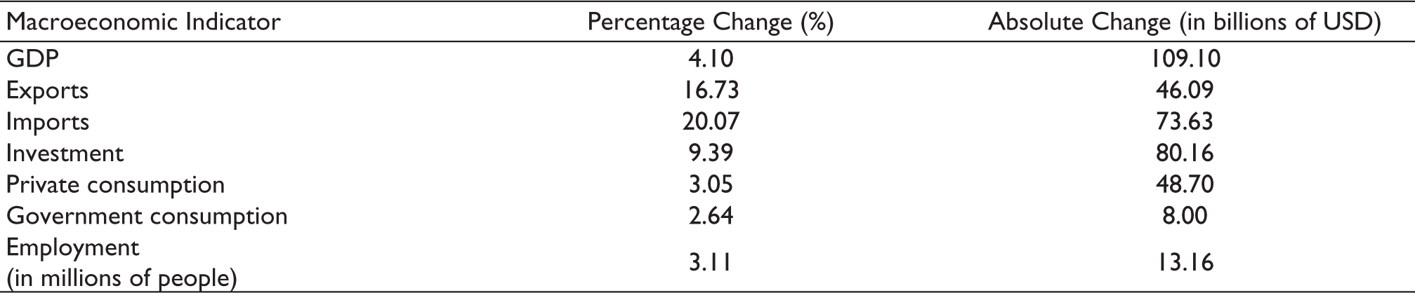
The model estimates that the GDP of India will increase at the rate of 4.10% (US$109.096 billion) by 2030 when tariffs and non-tariff measures are eliminated. Exports are estimated to increase at the rate of 16.73% (US$46.08 billion) and imports by 20.07% (US$73.625 billion) by 2030. The seven countries under study made up 30.57% of India’s exports in 2020 and 29.65% of imports in the same year. The model also estimates that the exports of India to these countries will increase by US$67.312 billion by 2030. This increase is higher than the increase in the aggregate exports of India revealing a trade diversion from the latter to the former. There is an increase in the export of several commodities including petroleum products (US$10.49 billion), chemicals (US$8.770 billion), apparel (US$6.756 billion), motor vehicles (US$3.41 billion), metal products (US$2.41 billion), iron and steel (US$2.02 billion), machinery and equipment (US$1.66 billion), electrical equipment (US$1.46 billion) and rubber and plastics (US$1.37 billion).
The model estimates that the imports to India from the seven countries under study will increase by US$124.893 billion and there is a significant increase in the import of agricultural commodities, such as oilseeds, rice, vegetables and fruits into India whose output and exports were estimated to decline.
To present recommendations on the offer and request for India during the negotiations, we present a novel approach using correlation analysis and k-means clustering. We first choose the following macroeconomic parameters and then use correlation analysis, a statistical measure that estimates the extent to which the variables are linearly related in order to improve the accuracy of our analysis. We use the k-Means clustering, an unsupervised machine learning algorithm to group data points in clusters and present recommendations on the list of commodities that India should offer to give up tariffs on and those commodities on which India should request its trade partner for tariff elimination. The analysis reveals that requesting full or partial tariff elimination on cotton textiles, apparel, other manufacturing, other food products, rice, leather, other crops, cattle meat, vegetables, fruits, motor vehicles and chemicals will be critical to increase its exports and achieve its export target by 2030.
The study is unique in several ways, most important of them is that it is the first exhaustive quantitative analysis of India’s ongoing FTAs and their estimated contribution to achieving the mission of Atmanirbhar Bharat. Second, the study has developed a novel methodology that combines the strengths of CGE modelling with machine learning methods. GTAP is a state-of-the-art, multi-region, multi-sector CGE model and has the ability to account for all the linkages and interactions happening in the economy, unlike the partial equilibrium models that have the ability to just focus on one sector, one region at a time. In the GDyn model that we use, time is treated as a variable, unlike other dynamic models that treat time as an index. By combining such an extensive model with an ML algorithm like k-means clustering, we present an exhaustive analysis of the impacts of the India’s FTAs.
The article is arranged in the following sections—the second section covers the literature review and the third section describes the methodology, model description and policy shocks. The fourth section covers the results and observations, followed by policy recommendations.
Literature Review
Role of FTAs in Promoting Economic Growth
Trade has been recognized as a key driver of growth and the composition of global trade has transformed over the years. Trade liberalization policies and technological advancements have opened up more economies to the global world (Erokhin, 2016). The literature aims to develop underpinnings for the vital role that the FTAs would play in enabling India to achieve its export target part of the Atmanirbhar Bharat campaign.
Promoting exports leads to the efficient allocation of resources in an economy, better economies of scale and employment generation while also enhancing manufactu- ring efficiency from increased capital formation and technological development (Bond et al., 2005; Shirazi & Abdul Manap, 2005). Trade allows healthy competition that drives technological growth, productivity enhancements and progress (Robinson, 2018).
Though developing economies struggle to cope up to the global trade scape due to issues, such as poor logistics and connectivity, competition from foreign players, etc., proper mitigation strategies through rules-based trade agreements help such countries accelerate growth. Developing countries that remain open to trade tend to grow faster and reduce poverty (World Bank, 2018). Countries that have liberalized trade grow at higher rates than those that are inward-looking (Grossman & Helpman, 1991). Trade liberalization facilitates quicker diffusion of knowledge and technology into developing countries from cheaper import of high-tech solutions and goods (Almeida & Fernandes, 2008).
A study on trade liberalization and firm productivity in India reveals that a reduction in trade protectionism and comprehensive tariffs in India in the 1990s lead to an increase in firms’ productivity and this is higher for private firms. It also shows how other attributes, such as regulations, labour laws, investment climate and so on do not influence the impact that trade liberalization policies produce on firm productivity (Topalova, 2004). Eliminating tariffs increases a country’s accessibility to potential markets and allows it to capture benefits that arise from economies of scale in the commodities they specialize in (Bond et al., 2005). Consumers also get access to wider goods and services, and they can benefit from higher quality and lower prices (Robinson, 2018).
Asian countries experienced higher levels of poverty in the 1960s and had an ample supply of inexpensive manpower. Their closeness to rapidly advancing economies and the efforts of WTO and GATT in promoting multilateralism anchored Asia’s growth in the 1990s (Kawai & Wignaraja, 2010). This was followed by a long period of trade expansion during which Asia leveraged its strengths to transform into a manufacturing hub with enhanced technological capabilities. Baldwin (2006) calls this ‘Factory Asia’ for it is an efficient factory that holds unimaginable price-quality ratios.
The benefits that countries can derive from trade agreements are also dependent on other factors that are exogenous to the trade agreements, such as economic structure, infrastructure, the magnitude of trade happening between countries, physical and institutional structure, geography, etc. (Gasiorek, 2019). Though a majority of studies reveal that trade agreements produce a positive there are studies that reveal how the outcomes of trade agreements on the members involved are uneven (Alba et al., 2008; Hannan, 2016; Jung & Cheolbeom, 2012). It is a common observation that a lot of times one or many parties to the agreements endure hardships from cheaper imports that push domestic industries into competition and losses. This calls for quantitative analysis of the Free Trade Agreements to be able to understand and evaluate the impacts of such agreements on the parties involved.
CGE Models Employed in the Analysis of Trade Deals and Dynamics
Trade agreements have always drawn the interest of researchers. We have curated literature on models used for trade policies in two categories—ex-post assessment of trade agreements that employ historical data, ex-ante prediction and assessments that most prominently use CGE methods to capture the impact of trade agreements before they come into effect.
Ravenstein (1885) used the gravity model to study immigration flows and Tinbergen (1962) used the gravity equation to study trade flows. Since then, the gravity equation has been a predominant econometric tool used to carry out an ex-post assessment of trade agreements. Anderson (1979) offered the much-needed theoretical underpinnings to the gravity equation while Poyhonen (1963), Geraci and Prewo (1977), Bergestrand (1985) and Deardorff (1995) popularized the usage of gravity framework to model trade flows and transportation costs.
A number of studies have come up extending the gravity model to cover key bilateral trade attributes, such as tariffs (Wall, 1999), infrastructure (Baita, 2020; Nordås & Piermartini, 2004), level of technological expertise (Hassani et al., 2015; Márquez-Ramos & Martínez-Zarzoso, 2010), exchange rates (Hasanov et al., 2011), trade in services (Kimura & Lee, 2006; Walsh, 2006), investments (Beugelsdijk & Zwinkels, 2010), foreign direct investment, etc. to increase the usability and viability of the model for trade policy analysis. In the Indian context, Bharti and Nisa (2021) used the gravity model to estimate the impact of the ASEAN FTA on the Indian merchandise trade. By using panel data of trade partners and by employing the generalized least squares (GLS), the study shows that the Indian trade is more dependent on the GDP of India and its partner countries, and other factors, such as geographical distance, common official language, common border, landlocked variables, etc. considered in the study have no significant impact on India’s trade. A study by Lohani (2020) to analyse the trade flows of India with the BRICS has used a gravity model augmented with time-invariant variables. The study has employed Poisson–Pseudo Maximum Likelihood (PPML) and it reveals that the export of goods is adversely affected due to a higher trade cost and calls for a negotiation with BRICS to increase trade flows. Saraswat et al. (2016), have used product space analysis to estimate the cost of FTAs and the study recommends that negotiating tariff removals and FTAs with countries that have higher trade complementarities and a greater margin of preference will benefit India.
Though gravity models and product space analysis offer a constructive framework to carry out an ex-post analysis of trade agreements using historical data, they do not provide a solid foundation for ex-ante evaluation of trade policies and trade agreements, which remains a challenge.
Ex-ante evaluation of trade agreements and trade policies uses partial equilibrium models and CGE models. There is literature evidence for the fact that applied general equilibrium models (AGE) have been used for the analysis of trade policies. Dervis et al. (1982) provide a theoretical underpinning for AGE models. Shoven and Walley (1992) and Kehoe and Kehoe (1994) used AGE models to estimate the impact of trade policies and agreements pursued by governments including the ex-ante evaluation of NAFTA.
Driven by the growing computational power, Hertel (1997) routed the importance of using CGE frameworks in trade policy analysis as such models capture the economy at a comprehensive level. Table 1 summarizes our survey of the GTAP studies used for ex-ante evaluation of the impact of FTAs.
GTAP Models Used in the Ex-ante Evaluation of FTAs.
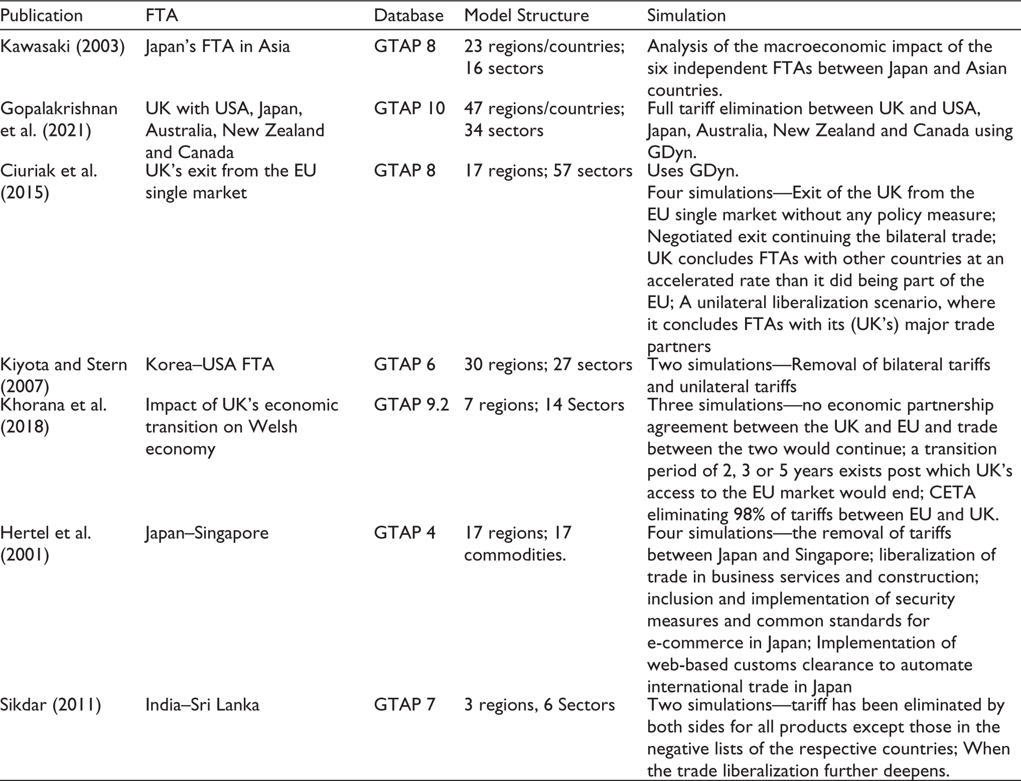
It should be noted that the handbook for trade sustainability impact assessment recommends using multi-region computable general equilibrium (CGE) to carry out an analysis of the direct effects of FTAs over time. A review of existing literature on the models that were used for the analysis of the impact of trade agreements demonstrates the advantages of using CGE models to capture the trade dynamics. The ability of such models to capture the inter-regional as well as inter-sectoral linkages serves an important role in trade policy analysis.
Methodology
A thorough, quantitative and comprehensive analysis of trade policies and trade agreements requires detailed analytical methods and frameworks that account for linkages, interactions and dynamics between various countries across the world. This is because, there exist linkages between not just different sectors of an economy, but these sectors are also linked to sectors of the rest of the world in the form of trade of finished goods, intermediate goods, capital goods, endowments and so on.
Model Description
Modelling of trade policies demands tools and frameworks that capture linkages and interactions happening at the national, regional and at global levels. Quantification of such linkages and impacts of different trade policies has been made possible by the evolution of analytical techniques, more so by the exponentially growing computational capacity.
General equilibrium models account for all the linkages between sectors of an economy including the forward and backward inter-industry linkages, as well as linkages between household expenditures and incomes. Events that take place in one industry/market may produce ripples in another industry. When accounting for trade agreements, such ripples must be accounted for, because there are chances that they feed back into the original market.
CGE models are ideal for analysing the impacts of trade liberalization policies and trade agreements as multiple countries and different sectors are involved and they must be effectively accounted for. The research employs GDyn, a recursive dynamic version of the GTAP, developed by the Center for Trade and Policy Analysis, Purdue University. The model produces the impact of a policy shock on national account aggregates, trade flows, industry output and prices, trade balances, factor inputs and prices, etc. For a technical description of the GTAP model, see Hertel (1997); for a discussion of the degree of confidence in CGE estimates, see Hertel et al. (2003). GTAP is a multi-region, multi-sector, CGE model built on the assumptions of perfect competition and constant returns to scale. The model was designed and developed by the Center for Global Trade Analysis, Purdue University. GTAP records the annual flow of goods and services for the global economy in a given base year. The model captures supply–demand linkages and equates them by accounting for changes in production, consumption, exports and imports. The behavioural equations in the model dictate production, private consumption, exports, imports and market-clearing conditions that equate supply with demand. Elasticity determine the substitution between various input and output parameters in the production and consumption behavioural equation.
GDyn is a multi-sector, multi-region CGE model and is an extension of the standard GTAP model as described and documented by Ianchovichina and McDougall (2000). The parameterization and applications of the model are documented by Ianchovichina and Walmsley (2012). GDyn is a powerful tool to study the economic impacts of the FTAs as they have the ability to capture the economy-wide impact of trade openness.
Generally, investment in a region depends on the rates of return and the balance that exists between savings and investment. In static CGE models, savings determine the investment, as the capital stock is fixed and not linked to changes in investment. But GDyn model accounts for short-term and medium-term differences in the rate of return between regions and lets the capital flow from countries that have a lower rate of return to those countries with a higher return. With time, in the long run, these differences even out resulting in long-run perfect capital mobility between regions.
Figure 1 offers a simplified structure of the original complex GTAP model. Here, the regional household receives factor payments (VOA) from different agents including private households, firms and the government for the supply of factors, such as land, labour and capital. The residual that remains after households’ expenditure on private consumption and government consumption is savings. The model is based on the Cobb–Douglas utility function that preserves the share of private consumption and government consumption. Global trust accumulates the savings and then distributes them across different regions as investments and this happens based on the rate of returns. This becomes a capital input to the firms that also use factor inputs (VOA) and intermediate inputs from domestic (VDFA) as well as imported (VIFA) to produce the output. This output caters to the consumption demand of private households (VDPA) and the government (VDGA), and also serves as an intermediate input to firms (VDFA). The private household and the governments can consume from the domestic output (VDPA/VDGA) as well as from imports (VIPA/VIGA), the consumption of which is governed by the Armington assumption.

The standard GTAP model provides a comparative static outlook of shocks including trade liberalization shocks in an economy. Drafting futuristic policies require models that have the potential to examine policy shocks over a period of time. GDyn models are appropriate when it comes to examining the policy dynamics for a particular time period. The model treats time as a continuous variable and subjects it to exogenous change with policy, technology and other demographic variables. The model carries all the attributes of the standard GTAP model—assumption of perfect competition, modelling of trade and transport margins, international capital mobility and ownership, disaggregated import usage by activity, Armington trade flows and non-homothetic consumer demands.
In GDyn, the experiment is compared against a counterfactual baseline scenario that captures the changes that are anticipated to happen in the normal run of an economy without accounting for the policy shock.
Baseline Projection
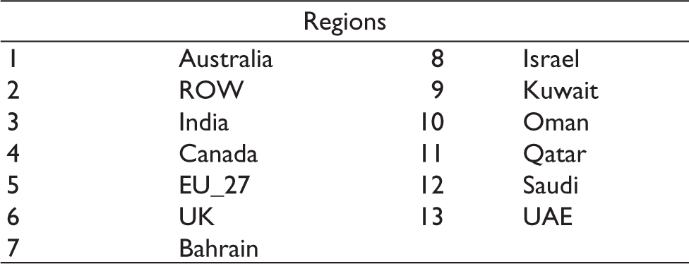
We use the latest publicly available GTAP database, version 10.0 (Aguiar et al., 2019) which is an exhaustive database covering 141 countries/regions and 65 sectors referenced to the year 2014. We have aggregated the same to 13 countries/regions and 56 sectors retaining all the countries and sectors that are an essential part of the Free Trade Agreements in which India is anticipating a conclusion. The regional aggregation is presented in Table 2.
Regional Aggregation.
The overall baseline assumption is that we let capital and labour be exogenous where capital is determined by the savings-investment mechanism and labour adjusts to keep the real wage rates fixed. Given that the latest available GTAP database is referenced to the year 2014, we scale the model to reflect the 2020 data, with data from the WEO database from International Monetary Fund. This is executed using GEMPACK from the Centre of Policy Studies (CoPS), Victoria University, Melbourne, Australia (Horridge, 2011).
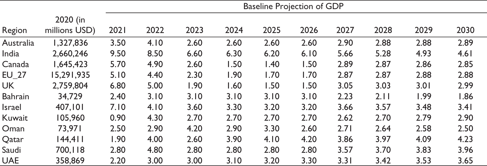
We then project the GTAP database to 2030 using historical data on GDP, population, unskilled and skilled labour. The projections are derived from reliable data sources and are explained as follows. The GDP projection for the years 2021–2026 is derived from World Economic Outlook from IMF estimates. The growth projection for the years 2027–2030 is taken from the IIASA database (IIASA, 2020), Socio-Economic Pathways and is scaled using differences that exist between IMF estimates and IIASA estimates for the years 2021–2026. It must be noted that the latest estimate from IMF covers the COVID impacts and the recovery that follows.
The baseline projections for population, unskilled and skilled labour are also derived from the IIASA baseline. The IIASA data accounts for the educational trends and human capital attainment that is seen in the shift happening from the unskilled labour force to the skilled labour force in some countries. Table 3 reveals the baseline projections of GDP employed in the article.
Baseline Growth Estimates.
Policy Shocks
To evaluate the impact of the Free Trade Agreements that India has signed with UAE and Australia, and is expecting to sign with the UK, the EU, Canada, Israel and the GCC, we made assumptions regarding the content of the agreement and the time period during which the agreements are expected to come into effect. We assume that all agricultural and industrial tariffs and non-tariff barriers are removed between India and the other countries that are expected to be a part of the agreements. Because the agreements of India with the UAE and Australia have already concluded, we assume that they come into effect from 2022, while the one with the UK concludes in 2023, those with the European Union and Canada in 2024 and that with Israel and GCC in 2025. The model is fed with sequential policy shock based on the anticipated time period of the conclusion of such agreements and their coming into force.
Novy (2013) developed a gravity redux method to estimate the Ad Valorem Equivalents (AVEs) of NTMs at an aggregate level. The study uses the benchmark between domestic trade within a country and bilateral trade between two countries with the extent of substitution between domestic trade and imports to estimate these AVEs. We extend this method to the sectoral level using GTAP services trade data. Then we assume that they are reduced to half by using a new variable we introduce in the model that reduces NTMs as if they were tariffs, without any direct implications for tariff revenue. The trade costs we estimate are residual in nature and may include some non-actionable NTMs, which we try to avoid lest we overestimate the gains from their reduction. So, we assume that the actionable NTMs are approximately half of all we estimate are eliminated in the services sector.
Offer-Request Analysis
To find the right basket of goods that could be offered and requested by India during the negotiation process, we adopt the following methodology. We pick the five most important economic indicators from the baseline results of our GTAP simulation. These include export value, output, employment, import and customs revenue. To improve the accuracy of the analysis we do the correlation analysis for the above-mentioned parameters. Based on the correlation coefficient, we ignore variables that have a high positive correlation.
We then use k-means clustering, a commonly used unsupervised machine learning algorithm to group data points based on the distance between them, the similarity and the pattern. The algorithm identifies the ‘k’ number of centroids initially and allocates the data points considered for study to the next nearest cluster.
And these clusters are then separated to identify commodities on which India should offer to reduce tariffs entirely (full tariff elimination) and those commodities for which the country should offer partial tariff elimination. The clusters also provide a set of commodities for which India should request full tariff elimination and moderate tariff elimination from the partner country during trade negotiations.
The idea behind selecting the commodities for India to offer tariff elimination for imports from the partner country is that the output of the commodity should remain high, imports should be low and customs revenue from the import of the commodity should be lower. This is keeping in purview that the tariff elimination should not increase imports and cut off a major portion of India’s customs revenue. On the other hand, the selection of a cluster of commodities from the partner country is based on the export value, output and import of that commodity. If the export value and output of a commodity are higher, India shall request tariff elimination for that commodity from the partner country. We select a cluster of commodities for bilateral elimination and this also looks at if losses from customs revenue due to the elimination of tariffs on that commodity can be offset by the increase in export of the commodity to that country.
Results
Change in GDP
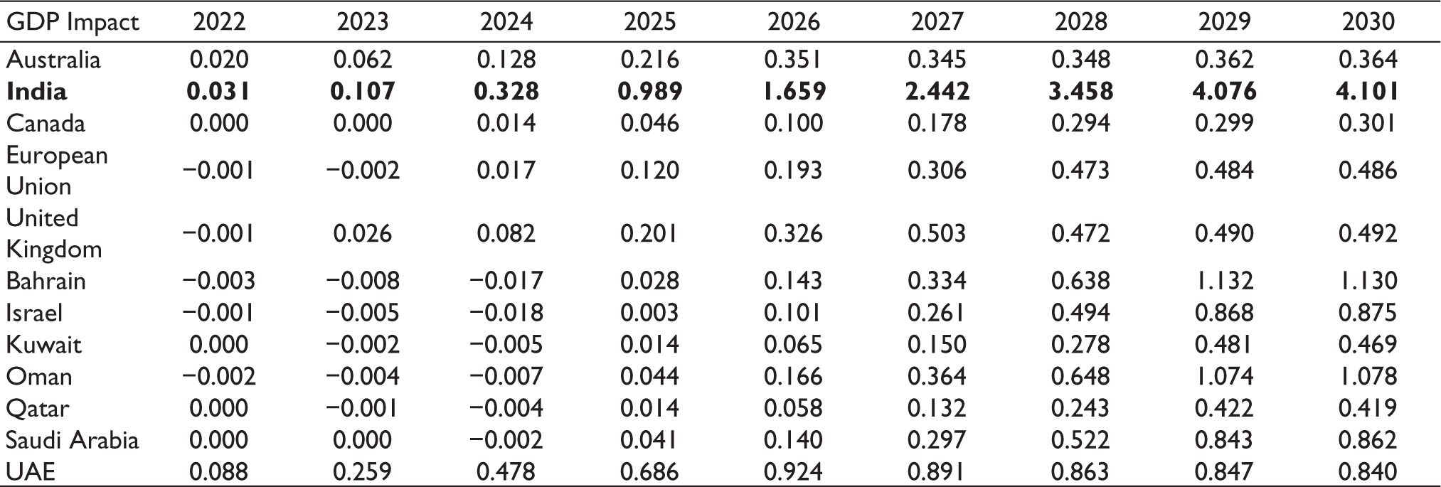
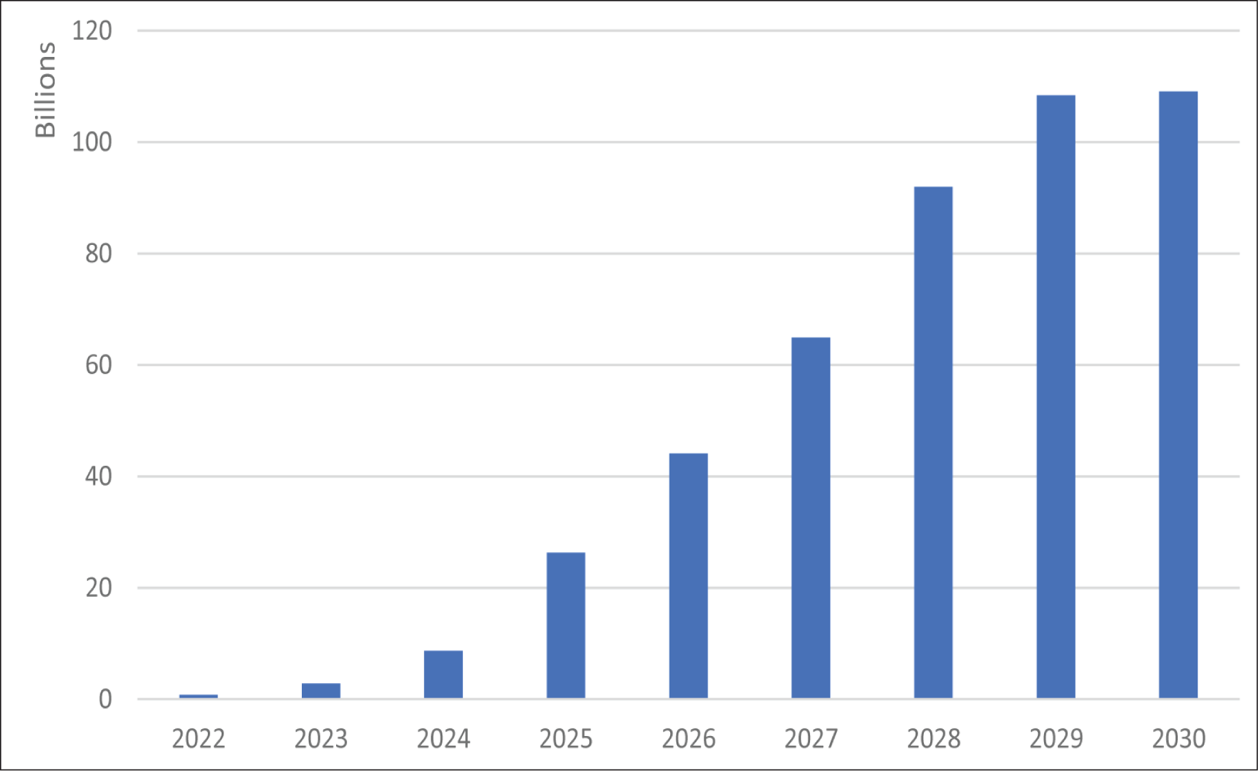
An analysis of the impact of the policy shocks on the GDP of India reveals that the GDP increases at the rate of 0.33% by 2024, 1.67% in 2026 and 4.10% by 2030 (in Table 4). In absolute terms, this amounts to US$8.725 billion by 2024, US$44.128 billion by 2026 and 109.096 billion by 2030. So, the elimination of tariffs and non-tariff barriers between India and UAE, Australia, Canada, UK, European Union, Israel and the GCC is estimated to add US$0.109 trillion to the Indian economy by 2030 (Figure 2).
Change in GDP Due to the Policy Shock.
A deeper analysis reveals that there is a gradual rise in GDP driven by an increase in exports and an increase in the output of manufacturing industries including construction, petroleum products, apparel, road transport, cotton and textiles, chemicals, real estate, milk products and so on. There is also a simultaneous decline in the output of machinery and equipment, crude oil, coal, electronics and the pharmaceutical industry. The output of some agricultural commodities including oilseeds, rice, vegetables and fruits, is estimated to decline. This is due to the reallocation of endowment commodities, such as land, labour and capital from the latter to the former.
The output of the construction and transport sectors shows a significant increase and this could be driven by an increase in infrastructure-related investments to promote more exports on the ground of trade liberalization. Tariff rates are significantly higher for the export of milk products from India to almost all the countries under study, particularly Canada and the UK. The increase in the output of milk products could be driven by the elimination of the tariffs between India and these countries. The same is the case with apparel, motor vehicles, cotton, leather, metal products, etc.
Change in Exports
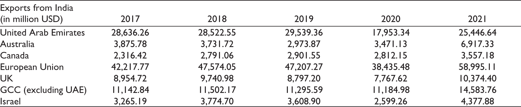
The seven countries/regions under our study which include Australia, Israel, Canada, UAE, the UK and the GCC, make up 32.89% of India’s total exports in 2019 during the pre-COVID period and about 30.57% in 2020. Of India’s aggregate exports, 13.95% are to the EU, 10.57% are to the GCC countries (including UAE), 2.82% to the UK, 1.25% to Australia, 1.02% to Canada and 0.94% are to Israel (inferred from Table 5).
Exports from India to Different Countries/Regions.
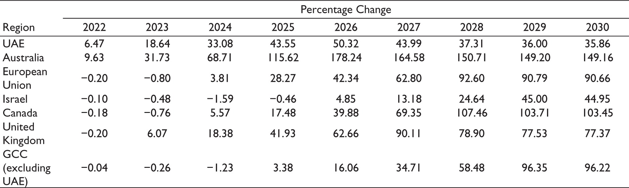
When the policy shock is fed to the model, it estimates that there will be an increase of 5.95% in the aggregate exports of India by 2025 which amounts to US$16.391 billion and 16.73% by 2030 which in turn amounts to US$46.089 billion. A region-wise analysis reveals that the export to UAE increases at the rate of 35.86% by 2030, that to Australia by 149.16%, the European Union by 90.66%, Israel by 44.95%, Canada by 103.45%, the United Kingdom by 77.37% and the exports from India to GCC increase by 96.22% by 2030 (Table 6). In terms of absolute change, the aggregate increase in total exports from India to all the regions and countries under study is US$67.312 billion. The reduced increase of aggregate exports of India when compared to the increase of exports to the countries under study reveals the diversion of exports that were earlier moving from India to the rest of the world, towards UAE, Australia, European Union, Israel, Canada, United Kingdom and GCC due to reduction of tariff and non-tariff measures.
Percentage Change in Exports from India to Different Countries.
In terms of absolute change, the highest increase in the exports from India is to the European Union which amounts to US$34.847 billion by 2030. The increase in exports from India to the GCC amounts to US$10.762 billion, to that of Australia by US$5.177 billion, the UAE by US$6.437 billion, Canada by US$2.909 billion and that of Israel by US$1.168 billion (Figure 3).

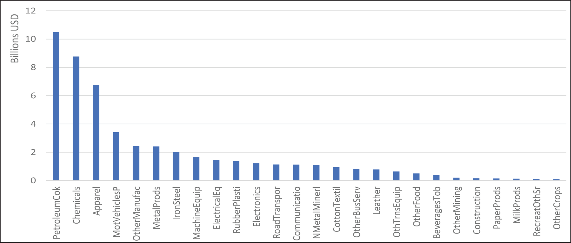
A deeper analysis of the change in exports at the sector level reveals that there will be an increase in the exports of petroleum products (US$10.49 billion), chemicals (US$8.770 billion), apparel (US$6.756 billion), motor vehicles (US$3.41 billion), metal products (US$2.41 billion), iron and steel (US$2.02 billion), machinery and equipment (US$1.66 billion), electrical equipment (US$1.46 billion), rubber and plastics (US$1.37 billion) and so on from India to other countries across the world (Figure 4). There is also a decrease in the export of pharmaceutical products, meat, rice, wheat, sugar, oilseeds and so on from India. Yet this decrease is offset by the higher increase in the export of manufacturing and other sectors. The estimated decrease in the export of agricultural commodities like rice and wheat comes from the re-allocation of land, labour and capital from these sectors to other efficient manufacturing sectors.
Change in Imports
Of the aggregate imports of India, the countries/regions under study make up 28.66% in 2017 and 30.36% in 2019 during the pre-COVID period and in 2020 it dropped to 29.65%. Country-wise data is attached in Table 7. Actually, 16.10% of India’s imports were from the GCC (including UAE), 9.07% of India’s imports in 2020 were from European Union, 1.97% from Australia, 1.28% from the UK, 0.75% from Canada and 0.48% from Israel (Table 7).
Imports into India from Different Countries/Regions.

When the model is subject to the trade liberalization shock, the aggregate import of India increases at the rate of 6.62% by 2025 and 20.07% by 2030. The increase in absolute terms amounts to US$24.383 billion by 2025 and up to US$73.625 billion by 2030. Among the seven countries and regions under study, the highest increase is from the UK, which in percentage terms is 179.12% by 2030, from Canada it increases by 178.82%, from the European Union, the imports increase by 148.83%, from Australia by 135.27%, from the GCC excluding UAE by 116.78% and from the UAE by 38.7% from the baseline by 2030 (Table 8).
Percentage Change in Imports into India from Different Countries.
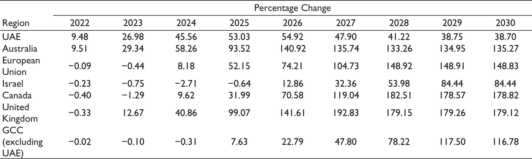
In absolute terms, the highest is from the European Union, where the import into India increases by US$49.70 billion, from that of GCC excluding UAE by US$41.292 billion, from Australia the increase amounts to US$9.824 billion, from the UAE it adds to US$9.248 billion, from the UK the increase is US$8.437 billion, from Canada it is US$4.908 billion and from Israel, the increase is US$1.479 billion (Figure 5). The aggregate increase in imports into India from these countries amounts to US$124.893 billion. There is a pronounced increase in the import of agricultural commodities, such as oilseeds, rice, vegetables and fruits whose output and exports were estimated to decline. To meet the domestic needs, the country imports more of these commodities when tariffs are liberalized.

The sectoral analysis reveals that at the aggregate level, there will be an increase in the import of machinery and equipment (US$9.072 billion), crude oil (US$7.154 billion), chemicals (US$4.941 billion), electronics (US$4.345 billion), electrical equipment (US$3.697 billion), motor vehicles and parts (US$3.528 billion), coal (US$3.438 billion), iron and steel (US$2.917 billion), other business services (US$2.728 billion), metal products (US$2.54 billion), cotton textiles (US$2.007 billion), paper products (US$1.773 billion) and so on (Figure 6). Almost all sectors witness an increase in imports except mineral and extraction sectors whose imports decrease by US$1.866 billion.

Other Macro-Economic Parameters
Offer-Request Analysis
As elaborated in the methodology section, we use correlation analysis and k-means clustering to identify commodities for which India should offer tariff elimination and those for which India should request tariff elimination. We chose the following macro-economic variables for this study—change in imports, exports, output, customs revenue and employment. The correlation analysis reveals that there is a high positive correlation between output and employment, and so we ignore the employment variables for k-means clustering and further analysis. So, we finally use the four significant indicators, output, export, import value and customs revenues. We then standardize each of these by using a z-score, which describes the position of that commodity in terms of its distance from the mean, when it is measured in standard deviation units.
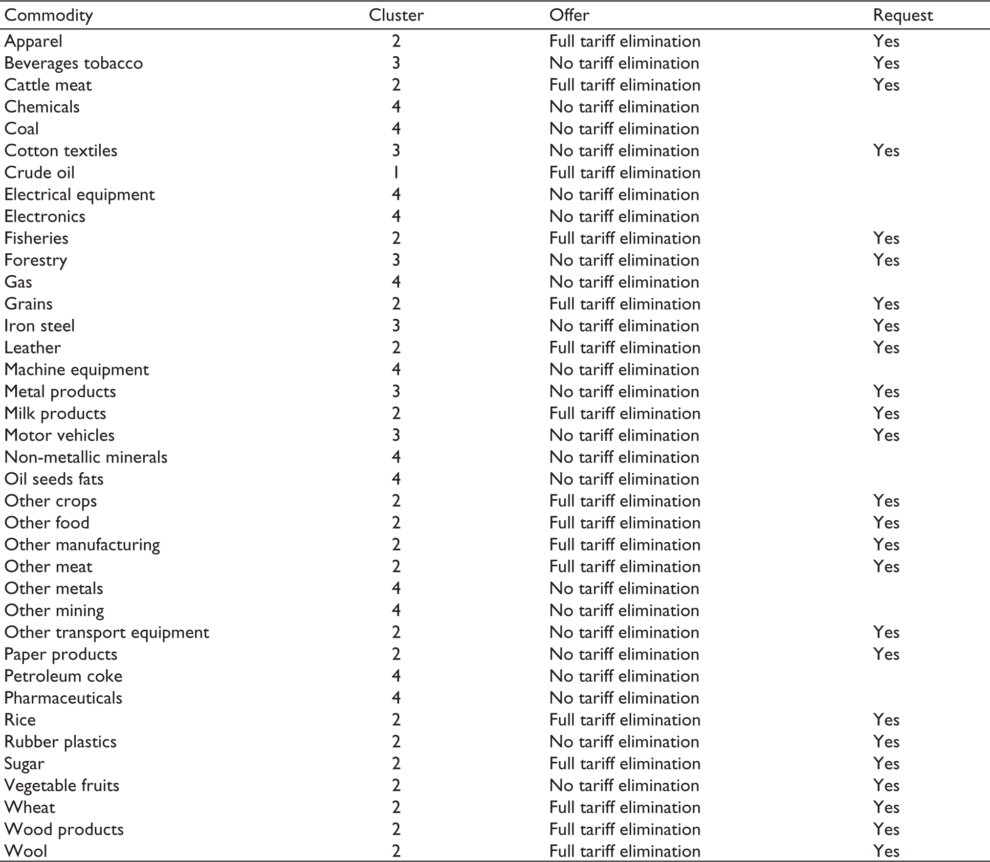
Using the standardized score for each of the commodities, we then proceed to k-means clustering. We identify four clusters—In the 1st cluster, we have grouped commodities that India can choose to eliminate tariffs and in the second, we have grouped commodities on which India should request for elimination of tariffs from partner countries and also offer for completion elimination of tariffs on their imports. The commodities in cluster 2 shall serve as a perfect choice for bilateral tariff elimination. For those commodities in cluster 3, it would be beneficial to India if it requests the elimination of tariffs on its exports to partner countries without offering tariff elimination on their imports. While for those in cluster 4, it would be critical to not offer tariff elimination to imports from partner countries while on the other hand whether India places a request for tariff elimination does not create a pronounced impact.
From Table 10, India should request for elimination of tariffs on the following commodities—apparel, beverages, cattle meat, cotton textiles, fisheries, forestry, grains, iron and steel, leather, milk products, metal products, motor vehicles, crops, food products, other manufacturing, transport equipment, paper products, rice, rubber plastics, sugar, vegetables, fruits, wheat, wood products and wool. Further analysis of the 10 essential commodities India should place for request using the absolute values reveal the following—cotton textiles, apparel, other manufacturing, other food products, rice, leather, other crops, cattle meat, vegetables, fruits, motor vehicles and chemicals.
Impact of Policy Shock on Macroeconomic Indicators.
Selection of Commodities Based on k-means Cluster.
Conclusion
As the study reveals, the execution of Free Trade Agreements between India and Australia, UAE, European Union, UK, Canada, Israel and the GCC, would add US$46.089 billion to India’s aggregate exports by 2030 (Table 9). The increase in exports as estimated by the model from India to the aforementioned countries is US$67.312 billion. Exports from India to the European Union increases by US$34.847 billion by 2030, to that of the GCC countries increased by US$10.762 billion, to Australia by US$5.177 billion, to the UAE by US$6.437 billion, to Canada by US$2.909 billion and that of Israel by US$1.168 billion. There is a significant increase in the export of petroleum products (US$10.49 billion), chemicals (US$8.770 billion), apparel (US$6.756 billion), motor vehicles (US$3.41 billion), metal products (US$2.41 billion), iron and steel (US$2.02 billion), machinery and equipment (US$1.66 billion), electrical equipment (US$1.46 billion) and rubber and plastics (US$1.37 billion).1
Under such circumstances, ensuring food security while also trying to become an export hub in manufacturing shall be a critical task for policymakers. The model also estimates a significant rise in imports particularly in the machinery, equipment and manufacturing sectors which in turn boosts the GDP, exports and employment in these sectors. A relatively lower increase in exports compared to the imports means that the GDP rise comes from consumption. So, to understand the commodities on which India should offer tariff elimination and in which it should not do so, we use a novel approach of combining statistical tools and machine learning algorithms. The study shows that India should not offer tariff elimination in the following commodities—beverages and tobacco, chemicals, coal, cotton textiles, electrical equipment, electronics, forestry, gas, iron and steel, machinery equipment, metal products, motor vehicles, non-metallic minerals, oilseeds and fats, other metals, other mining, transport equipment, paper products, petroleum coke, pharmaceuticals, rubber plastics, vegetables and fruits. On the other hand, it should request tariff elimination in the following commodities to the partner countries—cotton textiles, apparel, other manufacturing, other food products, rice, leather, other crops, cattle meat, vegetables, fruits, motor vehicles and chemicals. This could help India achieve its ambition of becoming an export hub as well as a manufacturing hub, while also minimizing the losses in customs revenue that could result due to tariff elimination for imports from its partner countries.
With the diminishing boundaries and rising levels of globalization, Free Trade Agreements have become a principal determinant of a country’s growth engine. India is no exception. Abolition of trade barriers while ensuring efficient distribution of resources and food security is the key to achieving its export vision and the mission of Atmanirbhar Bharat—a self-reliant economy.
Footnotes
Declaration of Conflicting Interests
The authors declared no potential conflicts of interest with respect to the research, authorship and/or publication of this article.
Funding
The authors received no financial support for the research, authorship and/or publication of this article.