



Abstract
The present study assesses the empirical performance of the new Keynesian IS model by estimating the standard as well as extended specifications of both the backward-looking and hybrid models in India over the period 1998Q1 to 2015Q4. It is found that the backward-looking IS model fits the data quite well in comparison with the hybrid model. The link between the policy rate and output gap appeared to be a bit stronger in the extended backward-looking IS model, as the interest rate coefficient is larger. Also, besides the interest rate, the real exchange rate, external demand and crude oil prices also have an impact on aggregate demand. The results suggest that the standard specification of the IS curve is inadequate to estimate the impact of the interest rate on aggregate demand and therefore a broader framework which accounts for additional variables besides the interest rate may be required.
“and contrary to what some economists might have predicted, the effort to integrate Keynesian-type elements into a dynamic GE framework has gone beyond providing rigorous micro-foundations to some pre-existing, though largely ad-hoc, framework”.
Introduction
Monetary policy formulated by the central bank has a crucial role to play in shaping the outcomes of macro-economic variables. The policy actions determine the consumption and investment decisions of individuals and firms, as changes in policy instruments, such as interest rates, directly affect the prices of financial assets and the expected returns from them (Gali, 2008b). The decisions of individuals and firms, in turn, have a bearing on output, inflation and employment in the economy. It is, therefore, essential to understand how policy actions determine nominal as well as real variables in the economy. Monetary theory provides us with an understanding of the process through which these impacts occur, termed the transmission mechanism of monetary policy. Against this backdrop, the development of a model for the monetary transmission mechanism, with clear micro-foundations in an individual optimisation framework, is essential to evaluate alterative monetary policies without being subject to the Lucas critique 1 . Also, the outcomes resulting from alternative policies can be evaluated by accounting for the preferences of private individuals which are given in the structural relations of the model (Woodford, 2003b).
The new Keynesian model has become a standard tool for monetary policy analysis among central bankers in recent times (Gali & Gertler, 1999; Goodfriend & King, 1997; Goodfriend, 2004; McCallum & Nelson, 1999a, 1999b; Rotemberg & Woodford 1999; Svensson & Woodford 2005; Walsh, 2010; Woodford, 2003a, 2003b). It has emerged as one of the most influential and prolific areas of research in macro-economics (Gali, 2008a). Its underlying framework synthesises the features of the real business cycles model and Keynesian theory. This framework provides the foundation for various models developed at central banks for simulation and forecasting. The new Keynesian model consists of three equations: the IS curve that defines output; the Phillips curve that defines inflation; and the Taylor-type interest rate rule that defines the conduct of monetary policy. There are number of studies that provide an excellent treatment of the model and its implications to monetary policy (Clarida, Gali & Gertler 1998, 1999; Gali, 2002, 2008a, 2008b; Gali & Gertler, 2007, Goodhart & Hofmann, 2005a, 2005b). Additionally, Carlin and Soskice (2005) depict a graphical framework of the models related to baseline new Keynesian theory that describes the interplay of inflation, the output gap and interest rate.
Many central banks around the world have successfully adopted inflation targeting as a new monetary policy strategy. Inflation targeting is based on an announced numerical inflation target, implementation of monetary policy that gives a major role to inflation forecast targeting, and a high degree of transparency and accountability. However, in practice, inflation targeting is never strictly enforced, but is always flexible, where the central bank aims at stabilising inflation around the target, as well as stabilising actual output around its potential. Thus, the target variables of a central bank include inflation as well as the output gap (Svensson, 2007).
The monetary policy framework in India has evolved over a period of time with the Indian central bank, the Reserve Bank of India (RBI) recently adopting a flexible inflation-targeting (FIT) framework, with consumer price index (CPI) inflation as a nominal anchor. It becomes essential, therefore, to employ a more comprehensive and complete model to analyse monetary policy transmission in India. The new Keynesian models provide us with the underlying framework essential for the conduct of monetary policy in inflation-targeting settings. The models imply that monetary policy that targets inflation at low levels will keep economic activity near capacity (King, 2000).
Since monetary policy is generally viewed as having a significant impact on output in the short-run, the analysis using the new Keynesian IS curve and Phillips curve has implications for monetary policy (Paradiso, Kumar & Rao, 2013). Most of the literature estimating new Keynesian models in India have focused on either the new Keynesian Phillips curve (Kapur, 2012; Mazumder, 2011; Mitra, Biswas & Sanyal, 2015; Patra & Ray, 2010; Paul, 2009; Singh, Kanakaraj & Sridevi, 2011) or the monetary policy reaction function (Hutchison, Sengupta & Nirvikar, 2010; Mohanty & Klau, 2004; Singh, 2010; Virmani, 2004). Very few attempts have been made to test the new Keynesian IS curve empirically. Further, the operating procedures for monetary policy in India have undergone significant changes in the last few years, such as the repo rate becoming the single policy rate to signal the policy stance and the call rate as the operating target of monetary policy (Reserve Bank of India [RBI], 2011). Since, most of the studies in the Indian context cover the sample period up to year 2011(prior to the implementation of the new operating procedures), their analysis misses on important policy occurrences in the post-2011 period, in which monetary policy was confronted with the dilemma of low growth and high inflation.
To fill this gap in the literature, the present study proposes to analyse the significant linkages in the monetary transmission process in India, following Goodhart and Hofmann (2005a, 2005b), Paradiso et al. (2013), Patra and Kapur (2010) and Kapur and Behera (2012). In doing so, the standard and extended specifications of the backward-looking as well as the hybrid versions of the new Keynesian IS model have been estimated and the role of the forward-looking and backward-looking components has been analysed. The rest of the article is organised as follows: second section provides an overview of the new Keynesian theory; a brief review of literature is given in third section; fourth section describes the model; fifth section covers the data, methodology, scheme of empirical estimation and the time path of the key variables under study; sixth section describes the results of the empirical estimation; and finally, seventh section concludes.
The New Keynesian Model: A Theory
The new Keynesian approach to macro-economics evolved in response to the Lucas critique and as an alternative to the competitive flexible price framework of the real business cycle (RBC) theory (Goodfriend & King, 1997). The models based on the new Keynesian theory combine the dynamic stochastic general equilibrium (DSGE) framework of RBC models with additional assumptions, such as monopolistic competition, nominal rigidities, and so on. The assumption of nominally rigid prices and wages in the new Keynesian models makes monetary policy non-neutral in the short-run. In the presence of nominal rigidities, a change in short-term interest rates by the central bank leads to a change in real interest rates, which eventually brings about a change in optimal consumption and in the investment decisions of households and firms which in turn determine output, inflation and employment in the economy. On the other hand, if long-run prices and wages adjust fully in proportion to the initial change in interest rates, monetary policy becomes neutral, that is, it has no real effect. The non-neutrality of money in the short-run makes monetary policy an important tool to intervene to enhance the welfare when distortionary shocks hit the economy (Gali, 2008b).
The assumption of infinitely living households maximising utility from consumption and leisure subject to the budget constraint, which was at the core of the RBC theory, is retained in the new Keynesian model. Representation of the supply side in the new Keynesian set-up is based on the assumption in Calvo’s (1983) model of inter-temporal optimal price setting behaviour by monopolistically competitive firms. Similarly, the demand side of the economy is modelled on the basis of the assumption of inter-temporal optimising behaviour of households. These assumptions signify the forward-looking Phillips curve and the IS curve, respectively. Since in the inter-temporal maximisation problem the behaviour of economic agents depend on the future as well as current course of monetary policy actions, the credibility of monetary policy gains importance (Clarida et al., 1999).
The new Keynesian model captures effectively the key channels of the monetary transmission process, namely, the interest rate channel, credit channel, exchange rate channel and asset price channel with great clarity (Anand, Dind & Tulin, 2014). The framework of the model describes the economy in three equations:
The first two equations characterise the aggregate demand and supply dynamics of the economy, respectively. The model is completed with the central bank reaction function, which summarises monetary policy response to economic developments. Interestingly, money has no explicit role in this model. In a simple form, the model depicts some important linkages among macro-economic variables. First, inflation and output are determined by aggregate demand, which is determined by the interest rates, and interest rates are in turn are set by monetary policy based on expected movements in output and inflation (Patra & Kapur, 2010). In addition, the relative importance of forward-looking versus backward-looking terms in the IS and Phillips curves also provides some important inputs into monetary policy formulation (Goodhart & Hofmann 2005a, 2005b). The standard version of the model includes only those variables, which are suggested by theory, whereas its extended version includes all other variables which may have an impact on output and inflation (Blanchard & Gali, 2007; Iacoviello, 2004). Thus, from the perspective of monetary policy, the model provides some important insights: the two important linkages, that is, the link between the output gap and the short-term real interest rate in the IS curve and the output gap and inflation in the Phillips curve, eventually measure the strength and effectiveness of monetary policy transmission.
Review of the Literature
Several national and international studies attempt to explore the important linkages in the monetary transmission process using the new Keynesian framework. However, the existing literature demonstrates quite diverse and contradictory results. While some studies provide evidence of strong and highly significant linkages in monetary transmission (Rudebusch & Svensson, 1999), others demonstrate insignificant linkages (Goodhart & Hofmann 2005a, 2005b). Similarly, evidence on the role of forward-looking expectations ranges from highly important (Gali & Gertler, 1999) to unimportant (Fuhrer, 1997).
Clarida et al. (1999) provide a more lucid and comprehensive explanation of the main structural relationships in the new Keynesian model and the design of optimal monetary policy in such a model in the presence of real-world complexities. Linde (2005) estimates hybrid versions of the IS and Phillips curves for the USA along with a Taylor Rule and identifies significant linkages between the output gap and short-term real interest rate in the IS curve. Rudebusch and Svensson (1999) estimate a backward-looking IS curve and Phillips curve for the US and find a significant negative impact of real interest rate on the output gap in the IS curve and a significant positive impact of the output gap in the Phillips curve. In two different studies, Goodhart and Hofmann (2005a, 2005b) estimate standard and extended specifications of the IS and Phillips curves for the G7 countries, the USA and the Euro area. Their results illustrate that the baseline specifications of the model fail to yield a significant link between the monetary policy instrument, output and inflation. However, the extended specifications of the model, which accounts for the impact of commodity prices on inflation and asset prices on the output gap, help restore important linkages in the monetary transmission process.
Paradiso et al. (2013) found similar results for Australia. Nelson (2001, 2002) estimates the backward-looking IS curve for the USA and UK, but fails to find any significant impact of the real interest rate on the output gap. The author refers to this finding as the IS puzzle, which may arise due to: (i) simultaneity bias arising from forward-looking monetary policy; (ii) mis-specification due to omission of forward looking elements; or (iii) mis-specification due to the omission of other determinants of aggregate demand. Fuhrer and Rudebusch (2004) estimate hybrid specifications of the IS curve for the USA using the conventional generalised method of moments (GMM) and maximum likelihood (ML). Their results show that the ML estimator is unbiased and yields a significant link between the real interest rate and the output gap. Ball (1998) and Svensson (2000), estimating open economy specification of the IS curve, found the exchange rate to be an additional variable influencing aggregate demand. Goodhart and Hofmann (2000) while estimating a small structural model for selected developed countries over the period from 1973 to 1998 found that financial variables, such as property prices and share prices, have a significant impact on the output gap. Hence, besides the short-term real interest rate, the potential impact of several other financial variables on aggregate demand should be taken in to account in monetary policy formulation.
There are a few studies in the Indian context which attempt to use the complete new Keynesian model to examine monetary policy transmission (Anand et al., 2014; Bhattacharya & Patnaik, 2014; Kapur & Behera, 2012; Patra & Kapur, 2010; RBI, 2002). In addition, several studies attempt to estimate at least one of the blocks of the new Keynesian model separately, that is, the Phillips curve equation (Kapur, 2012; Mazumder, 2011; Mitra et al., 2015; Patra & Ray, 2010; Paul, 2009; Singh et al., 2011) and the monetary policy reaction function in the form of a Taylor-type rule (Hutchison, Sengupta & Singh, 2010; Mohanty & Klau, 2004; Singh, 2010; Virmani, 2004). As far as the IS curve is concerned, very few attempts have been made to test it separately.
The RBI (2002, 2004) estimates a purely backward-looking IS equation for India using annual data, with reasonably robust empirical results. The estimated equation shows a significant impact of the real interest rate and international oil prices on aggregate demand. Patra and Kapur (2010) estimate various specifications of the IS curve for India using quarterly data from 1996 to 2009. The estimated IS equation is part of three equationsin the new Keynesian model. Their empirical evidence suggests that of these, the augmented backward-looking IS model, which includes additional variables such as the real effective exchange rate and real world exports, provides the best fit. It is found that the interest rate impacts aggregate demand after a lag of three quarters and inflation after a lag of seven quarters. Bhattacharya and Patnaik (2014) introduce a semi-structure new Keynesian open economy model for monetary policy analysis in India using quarterly data from 1996 to 2013. Their calibrated parameter values in the IS equation indicates a significant impact of the real interest rate and real exchange rate on the output gap. Anand et al. (2014) estimate a variant of the small ‘new Keynesian’ macro-economic model with rational expectations to analyse the dynamics of inflation and monetary transmission in India from 1996Q1 to 2013Q4. Their estimated aggregate demand (IS) equation shows a significant impact of the real interest rate gap, the real exchange rate gap and the foreign output gap on the output gap. Also, the coefficient on the lagged output gap is found to be greater than that on the lead output gap. Kapur and Behera (2012) examine the monetary policy transmission mechanism in India over the period from 1996 to 2012 using a small macro-model with new Keynesian features. Their estimated backward-looking IS equation indicates that the interest rate channel of monetary transmission is effective in the Indian context and the magnitude of the impact on growth and inflation is comparable to that in major advanced and emerging economies.
The existing literature provides some mixed and contradictory results regarding empirical estimation of the IS curve in the new Keynesian framework. Further, there appears to be limited empirical evidence on the IS curve compared to the other two equations in the new Keynesian model.
The Model
Theoretical Perspective
The new Keynesian model reduces the economy to a three-equation system comprising an aggregate supply or Phillips curve, an aggregate demand or IS curve, and the monetary policy reaction function. In the model, monetary policy affects the output gap through the IS curve in the first stage and then inflation through the Phillips curve in the second stage. The model, grounded in dynamic general equilibrium theory, is an improvement over the traditional IS-LM model in two contexts: First, the IS curve and Phillips curve are based on micro-economic foundations and take into consideration forward-looking economic behaviour; and second, the monetary policy reaction function emulates the operating procedure of modern central banks more accurately (Patra & Kapur, 2010).
The new Keynesian IS curve denotes real aggregate demand as a negative function of the real interest rate, giving scope for monetary policy to steer aggregate demand by exercising control over the interest rates and consumption. This IS curve, which is dynamic, is derived by log linearising the consumption Euler equation (see Equation 1) assuming inter-temporally optimising households, which follow the principle of consumption-smoothing with respect to their lifetime income.

In Equation (1) all the variables are in logs; yt is the output gap, E t yt+1 is the current period’s expectation of the next period’s output gap, it is the short-term nominal interest rate, and E t πt+1 is the current period’s expectation of the next period’s inflation rate; εt is the unanticipated aggregate demand shock with mean zero and no serial correlation. It is the ex-ante real interest rate defined as it – E t πt+1, that is used in the IS equation. A negative coefficient of the ex-ante real interest rate signifies inter-temporal interest elasticity of substitution between present consumption and consumption in the next period. Since inter-temporal optimising households prefer to smooth their consumption in response to higher income in future, expectations of higher future output impel them to consume more in the current period, which leads to an increase in aggregate demand and output. Current period output, therefore, depends on expected future output and the real interest rate. With forward iteration of Equation (1), it can be shown that the output gap depends on the current as well as the expected future path of the real interest rate and the demand shock. It denotes that in the presence of rigidities (prices, wages, and so on,) and, thereby, control of monetary policy over the short-term real interest rate, expected and current policy actions will affect aggregate demand (Clarida et al., 1999).
Theoretically, the new Keynesian IS curve and Phillips curve are purely forward-looking. Since, the purely forward-looking models fail to attain the robust estimates empirically, many researchers use the backward-looking and hybrid versions of the model to estimate the lagged and persistent response of inflation and output to monetary policy (Goodhart & Hofmann 2005a, 2005b; Peersman & Smets 1999; Rudebusch & Svensson, 1999; Rudebusch, 2002). 2 To introduce the backward-looking terms in the IS and Phillips curves, Gali and Gertler (1999) assume that a fraction of price setters apply a rule-of-thumb adjustment and simply adjust prices to past prices and inflation. Hence, the expected future values of inflation and the output gap can partly be approximated by lag polynomials (Goodhart & Hofmann, 2005b). Moreover, though the backward-looking terms in the IS curve are inconsistent with theory, they can be introduced by assuming habit persistence the in consumption behaviour of households, so that households’ utility also depends on lagged consumption (Fuhrer, 2000).
The empirical findings on the backward-looking and hybrid IS models are mixed. 3 Studies estimating a backward-looking IS curve found an insignificant relationship between the real interest rate and output gap (Goodhart & Hofmann, 2005a, 2005b; Nelson, 2002). It is argued that omitting variables which may have a significant impact on aggregate demand, besides the interest rate, could be the main cause of an insignificant real interest rate coefficient, as the interest rate effects are transmitted to aggregate demand via these variables (Goodhart & Hofmann, 2005a). To account for this, several studies augmented the baseline backward-looking and hybrid models with additional variables and found a significant coefficient on the real interest rate (Hofmann, 2001; Nelson, 2002; Svensson, 2000).
Against this backdrop and given the limited literature on new Keynesian models under Indian conditions, the present study attempts to examine the links in the monetary transmission process by factoring in and comparing the role of forward-looking vis-à-vis backward-looking elements in the IS curve under a new Keynesian characterisation of the Indian economy. In doing so, four specifications of the purely backward-looking and hybrid versions of the new Keynesian IS curve have been estimated:
The baseline backward-looking IS curve:
The extended backward-looking IS curve:
The hybrid IS curve:
The extended hybrid IS curve:




Where yt is the output gap, it is the short-term nominal interest rate, πt is the inflation rate, εt is the aggregate demand shock, E t yt+1 is the current period’s expectation of the next period’s output gap, E t πt+1 is the current period’s expectation of the next period’s inflation rate, and it – E t πt+1 is the ex-ante real interest rate (rt). All the additional variables are listed in the appendix.
In the standard specifications (Equations 2 and 4) only those variables which are directly suggested by theory are included in the model. On the other hand, in the extended specifications (Equations 3 and 5), all variables that embody significant demand-side effects, such as the exchange rate, external demand, crude oil prices, non-food credit and BSE stock prices, have been included in the models. The inclusion of additional variables in the equations here is ad-hoc, but can be rationalised by appropriate extensions of the basic theoretical models (Blanchard & Gali, 2007; Goodhart & Hofmann, 2005b; Iacoviello, 2004).
The present study estimates different specifications of the IS curve for India using quarterly data over the period from 1998Q1 to 2015Q4. While data on the GDP series, non-food credit, weighted average call rate, BSE Sensex, REER (36-currency trade weighted) and NEER (36-currency trade weighted) have been sourced from the RBI’s Handbook of Statistics on the Indian Economy, data on the CPI-IW (Inflation) have been sourced from the Central Statistics Office’s (CSO) website; data pertaining to crude oil price index and world exports have been taken from the IMF’s International Financial Statistics.
Most studies on India use the Index of Industrial production (IIP) as an activity variable, which is inappropriate as the IIP forms only one-fifth of total GDP (Patra & Kapur, 2010). The present study, therefore, uses real GDP as the activity variable. The output gap is calculated by de-trending the seasonally adjusted GDP using the Hodrick-Prescott filter, where λ was set equal to 1600. All the variables except the call rate were seasonally adjusted using X-13 ARIMA and were used in the first difference. For its methodology, the present study follows Clarida et al. (1998, 2000),Goodhart and Hofmann (2005a) and Paradiso et al. (2013), to estimate the equations by the GMM in view of the leads of the explanatory variables being used and potential endogeneity of the variables. However, the purely backward-looking models are estimated by the OLS method.
The Scheme of Empirical Estimation
Testing the data for stationarity;
Estimating the baseline backward-looking model (OLS);
Estimating the extended backward-looking model (OLS);
Estimating the hybrid model (GMM); and
Estimating the extended hybrid model (GMM)
Theoretically, the specification of the IS curve includes variables measured in real terms. Since the purpose of this study is to estimate the IS curve as specified in the new Keynesian theory, it estimates the IS equation using real variables, first. However, to supplement the analysis only the backward-looking IS equation has been re-estimated using nominal variables as it was empirically found that the backward-looking model fits the data well.
The Path of the Variables Under Study
The Output Gap
In Figure 1, the output gap has been expressed as a percentage of potential output. The positive output gap between late-1999 and early-2000 and late-2010 and early-2013 indicates periods of overheating. The output gap is seen to be negative over few quarters of 2014–15, denoting slack in the economy in recent periods, due to a weak global demand. It can be seen that the output gap reaches its peak of around 3 per cent in 2007Q4, just before the financial crisis broke out in the USA. However, in the subsequent period (especially in 2008), the output gap turns negative due to the repercussions of the financial crisis and was seen to be narrowing in late-2009.
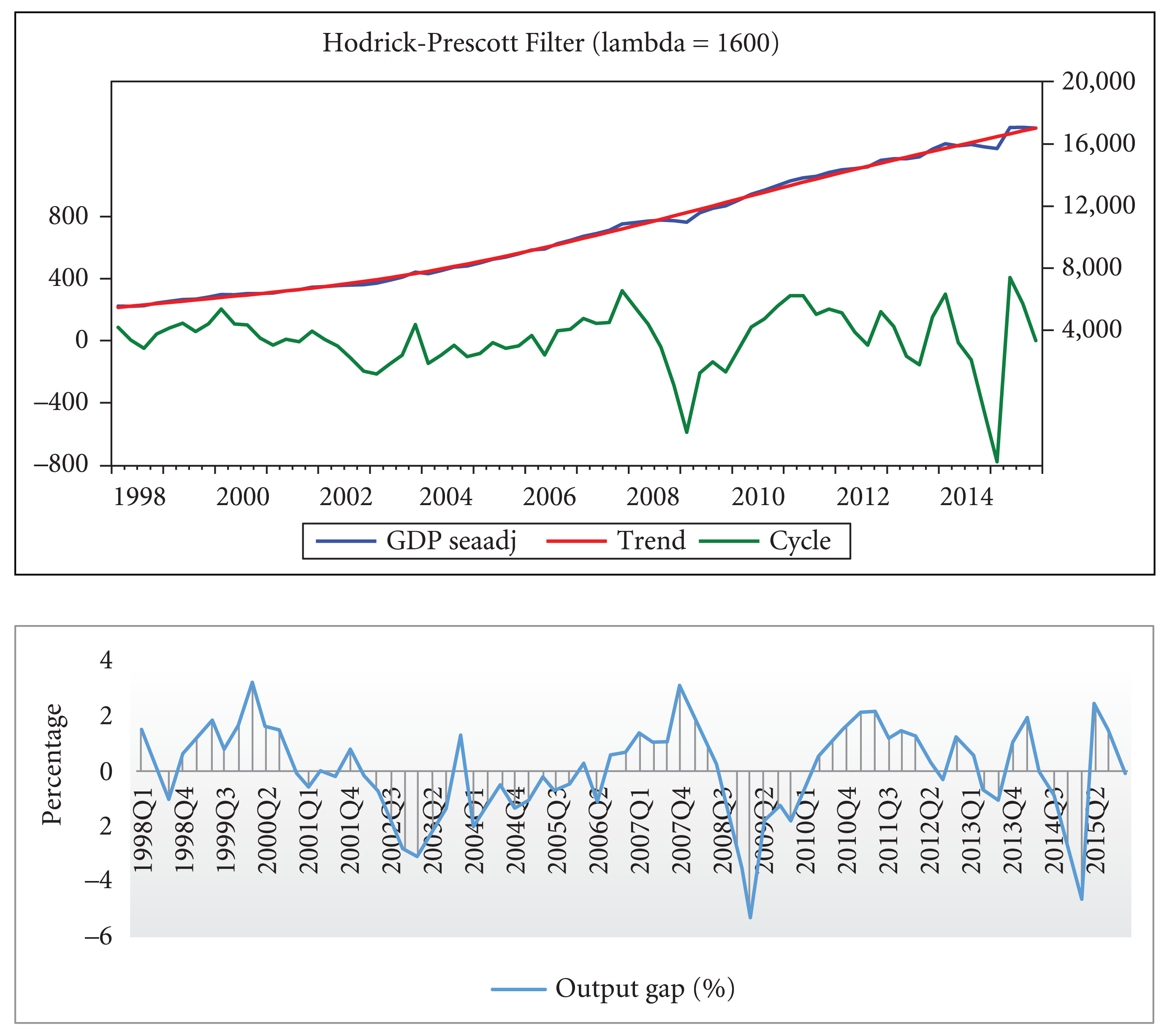
The monetary policy framework and operating procedure in India have undergone significant changes during the sample period. The liquidity adjustment facility (LAF) 4 was introduced in the early-2000s to manage day-to-day liquidity in the system through repo and reverse repo operations. Monetary policy signals were provided through the repo and reverse repo rates. Hence, during excess liquidity conditions, the reverse repo rate was the effective policy rate, whereas in tight liquidity conditions, the repo rate was the effective policy rate. Therefore, the policy rate switched between the repo and reverse repo rates (Patra & Kapur, 2010). As a result, there was a need for a single rate to signal the monetary policy stance, hence the monetary policy operating framework was modified and the new operating framework came into effect in May 2011. In the new framework, the repo rate was made the single independently varying policy rate to signal the policy stance, and the weighted average overnight call money rate was explicitly recognised as the operating target of monetary policy, as monetary policy signals were transmitted to this segment faster than to the other money market segments (RBI, 2011). The present study, therefore, uses the weighted average call rate as a proxy for the policy rate, as it has been moving in tandem with the effective policy rate, that is, either the repo or reverse repo rate, depending on prevailing liquidity conditions.
Figure 2 depicts the paths of the nominal and real call rates over the sample period. Fluctuations in the call rate signify different phases of expansionary and contractionary monetary policy. Monetary policy was highly expansionary in the post-crisis period, as can be seen from the steep fall in the call rate to provide a stimulus to the economy. However, the monetary policy stance shifted to a tightening phase in the post-2009 period, as inflation posed a major threat to the economy. Along with the nominal interest rate, the real interest rate is an important determinant of consumption and investment decisions. The real call money rate is computed by adjusting the nominal rate for CPI inflation. The path of the real rate depends on the underlying nominal interest rate and inflation dynamics in the economy. Even though monetary policy was in contractionary mode post-2010, the real interest rate was negative over the span due to high inflation. The real interest rate has remained around 2 per cent in recent years.

The Unit Root Tests
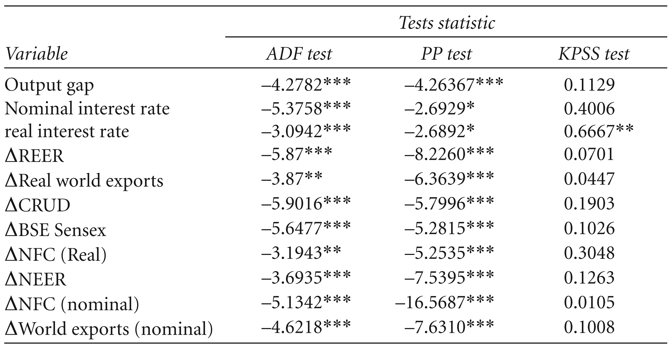
All the variables were tested for stationarity using the augmented Dickey–Fuller (ADF), Phillips–Perron (PP) and Kwiatkowski–Phillips–Schmidt–Shin (KPSS) tests. While the call rate was found to be stationary in the level form, all the other variables were non-stationary and therefore used in the first difference. Non-food credit in nominal terms was stationary in the second difference. The results of the unit root tests are shown in Table 1 in the appendix.
The Baseline Backward-looking IS Model
In empirical estimation, the forward-looking theoretical IS curve is often approximated by a backward-looking specification (Fuhrer & Moore, 1995; Rudebusch, 2002; Rudebusch & Svensson 1999). Following Goodhart and Hofmann (2005a) and Paradiso, Kumar and Rao (2013), the baseline backward-looking IS model has been specified in the form:

The results of the empirical estimation of Equation (6) by OLS are shown in Table 1. It is important to note that Equation (6) is estimated by including one lag of the real interest rate at a time. After re-estimating the equation with different lags of the real interest rate, it is found that the real interest rate co-efficient is significant at the fourth lag 5 . The real interest rate (rt) on the right hand side of the equation represents the monetary transmission mechanism, which in the case of many central banks may include nominal interest rates, ex-ante real short and long rates, exchange rates, as well as direct credit quantities (Rudebusch & Svensson, 1999).
OLS Estimates of the Baseline Backward-Looking IS Curve (real variables)
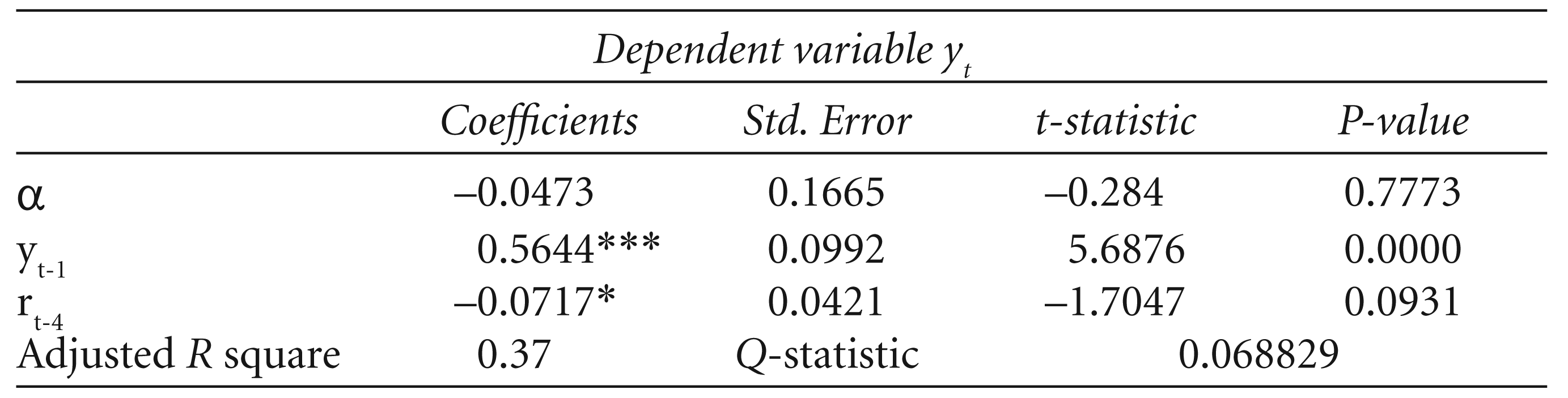
(ii) The Q-statistic denotes the Box-Ljung test statistic for residual autocorrelation.
The results show that both the lagged output gap and real interest rate (rt) are significant at the 1 per cent and 10 per cent levels, respectively, and have the expected sign. The real interest rate has a negative impact on the output gap. An increase in the policy rate by 1 per cent leads to narrowing of the output gap by 0.07 per cent after a lag of four quarters. 6 The coefficient on the one-period lagged output gap is highly significant and positive at 0.56, indicating the output gap inertia. The diagnostic test results indicate no serial correlation in the residuals.
Even though the results suggest a significant link between the policy rate and output gap, the transmission of policy impulses to output is not as strong (the coefficient is a meagre 0.07) and subject to a lag of four quarters. Several factors are responsible for the weak transmission of monetary policy to output in India: The banking system is still the major source of borrowing and is dominated by public sector banks. Despite several rate cuts by RBI and a corresponding fall in the short-term rates, banks fail to pass on these rate cuts as they are reluctant to reduce their lending rates. Thus while bank lending rates have gone down, the decline is not commensurate with the policy rate cuts (Rajan, 2016). However, the marginal cost of funding approach 7 recently implemented by the RBI is a positive step and may help bring desirable results. It is possible that other variables apart from the interest may also determine the output gap and the baseline backward-looking model has been augmented to account for this.

If aggregate demand is also determined, other variables besides the interest rate and if interest rates are a function of these variables, then the estimated interest rate coefficients will be biased towards zero (Goodhart & Hofmann, 2005a). To asses this argument, the baseline IS model has been augmented with additional variables besides the real interest rate, such as the real effective exchange rate (REER), real non-food credit, BSE Sensex, real world exports (as a proxy for external demand) and the crude oil price index. Table 2 reports the results of the OLS estimation of Equation (7).
The real policy rate (rt) has a significant negative impact on the output gap after a lag of six quarters (Table 2). However, the interest rate coefficient at -0.09 is slightly higher than the coefficient in the baseline backward-looking IS model. This indicates that after allowing for additional variables which may influence aggregate demand in the model, the link between the real policy rate and the output gap has become a bit stronger. A 1 per cent increase in the real interest rate now leads to a fall in the output gap by 0.09 per cent. Besides the interest rate, the REER, external demand and crude oil prices also have significant and expected impacts on the output gap. 8 An appreciation of the real exchange rate has the expected contracting impact on real activities: an appreciation of the rate by 1 per cent results in a reduction into the output gap by 0.13 per cent after a lag of seven quarters. Similarly, external demand as proxied by real-world exports has a significant positive impact on economic activities: a 1 per cent increase in external demand leads to a widening of the output gap by a robust 0.5 per cent after three lags. An increase in the crude oil price index also has a significant negative impact on the output gap. The coefficients on the BSE Sensex and real non-food credit are insignificant. Clearly, apart from the interest rate, these additional variables also determine aggregate demand and therefore can play a significant role in policy formulation. The Q-statistics denotes no serial correlation in the residuals.
OLS Estimates of the Extended Backward-Looking IS Model (real variables)

(ii) The Q-statistic denotes the Box-Ljung test statistic for residual autocorrelation.
The estimated baseline backward-looking model may not be structural, so this study estimated the standard and extended specifications of the hybrid IS model. 9

Equation (8) shows the specifications of the standard hybrid model. In addition to the lag in the output gap, it includes the current period’s expectation of the next period’s output gap (E t yt+1) to avoid downward-biased interest rate elasticity which leads to the IS puzzle (Nelson, 2001). Also, instead of the ex-post real interest rate, an ex-ante real interest rate-defined as the current period’s short-term nominal interest rate less the current period’s expectation of the next period’s inflation rate (E t πt+1)-is used. Equation (8) is estimated by the GMM using two lags of the output gap, four lags of the ex-ante real interest rate, and the intercept as instruments. The results of the GMM estimates are given in Table 3.
GMM Estimates of the Standard Hybrid Model (real variables)
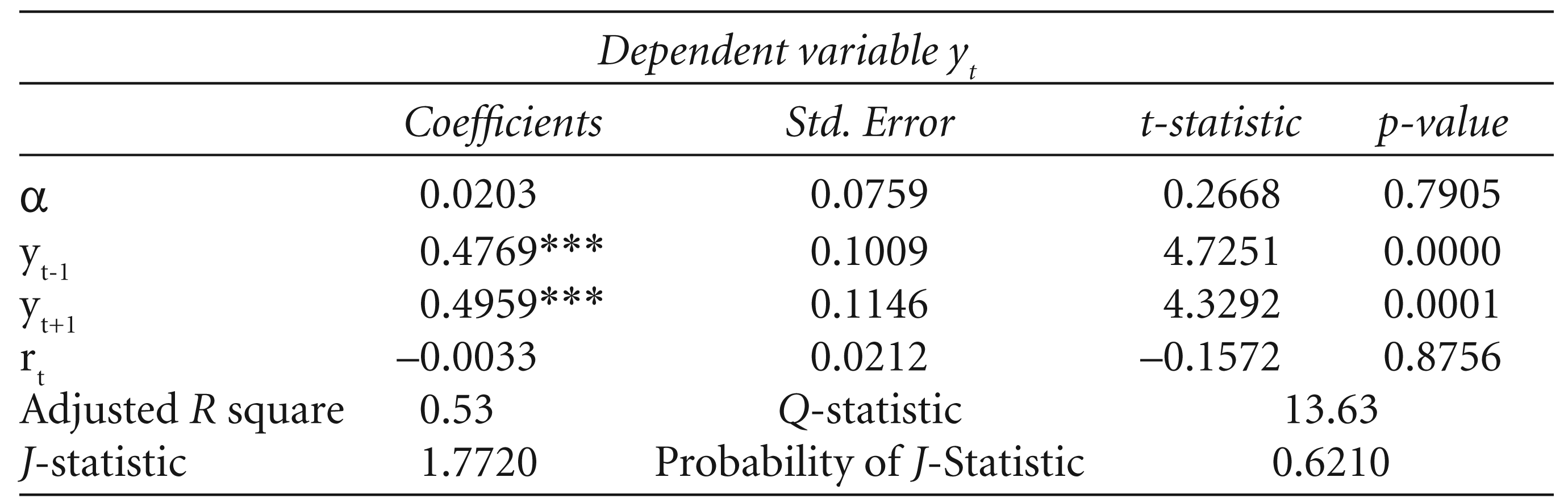
(ii) The Q-statistic denotes the Box-Ljung test statistic for residual autocorrelation.
(iii) The J-statistic and its probability value have been tested for over-identifying restrictions.
The t-statistics were calculated based on heteroscedasticity and autocorrelation robust Newey-West standard errors. The Hansen’s (1982) J-test statistic indicates that the selected instruments are valid. The results show that the link between the policy rate and output gap does not exist in the hybrid model, as the real interest rate coefficient is insignificant. The coefficients on the one-quarter-ahead expected output gap and the lagged output gap are significant and positive, with the coefficient on the lead output gap having a greater magnitude than the coefficient on the lag. It is, therefore, the expected future output gap that impacts the current output gap more than the past output gap. The Q-statistic indicates a serial correlation in the residuals. Since the standard hybrid model rejects the existence of a significant link between the policy rate and the output gap, the hybrid model has been augmented to control for variables that may influence aggregate demand.

The baseline hybrid model is augmented to control for additional variables besides the real interest rate, such as the REER, real-world exports (as a proxy for external demand), the BSE Sensex, crude oil price index and real non-food credit. Equation (9) was estimated by the GMM, using three-to-seven lags of the ex-ante real interest rate; four lags of real non-food credit, the BSE Sensex, crude oil price index, and external demand; two lags of the output gap; and six lags of the REER, and a constant as instruments (Table 4).
The results of the estimation show that the interest rate coefficient is again insignificant in the augmented hybrid model. However, the coefficients on the lagged and lead elements of the output gap are significant, with the coefficient on the lagged element of greater magnitude than on the lead element. The REER, real non-food credit, external demand and crude oil price index have an expected significant impact on the output gap. While an appreciation of the real exchange rate by 1 per cent reduces the output gap by 0.15 per cent, an increase in external demand by 1 per cent leads to a widening of the output gap by 0.57 per cent. The J-statistic indicates that the instruments specified are valid. The Q-statistic indicates no serial correlation in the residuals.
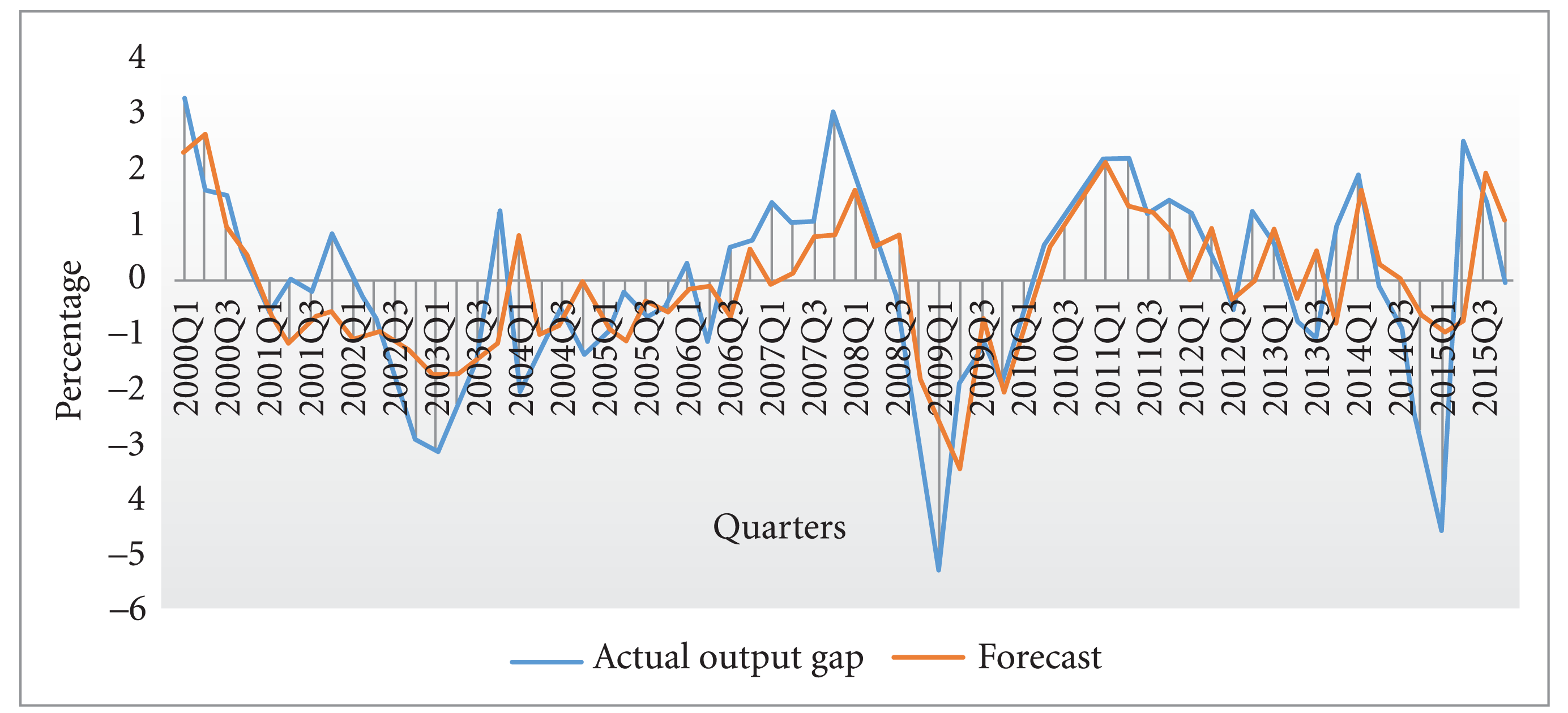
Among all the estimated specifications of the IS model, it appears that the link between the policy rate and real activity, an important link in the monetary policy transmission process, is present in the backward-looking specifications of the IS model. The hybrid models, which include both forward-looking and backward-looking elements, fail to survive empirically. From among all the specifications of the IS model, it is found that the backward-looking extended IS model fits the data quite well. This model also satisfies all the diagnostic tests on the residuals, so it is used in the model simulation. Equation (7) exhibits a satisfactory performance in terms of in-sample forecasting. The model tracks the actual data fairly well by capturing the various turning points in the actual series (Figure 3).
GMM Estimates for the Extended Hybrid Model (real variables)
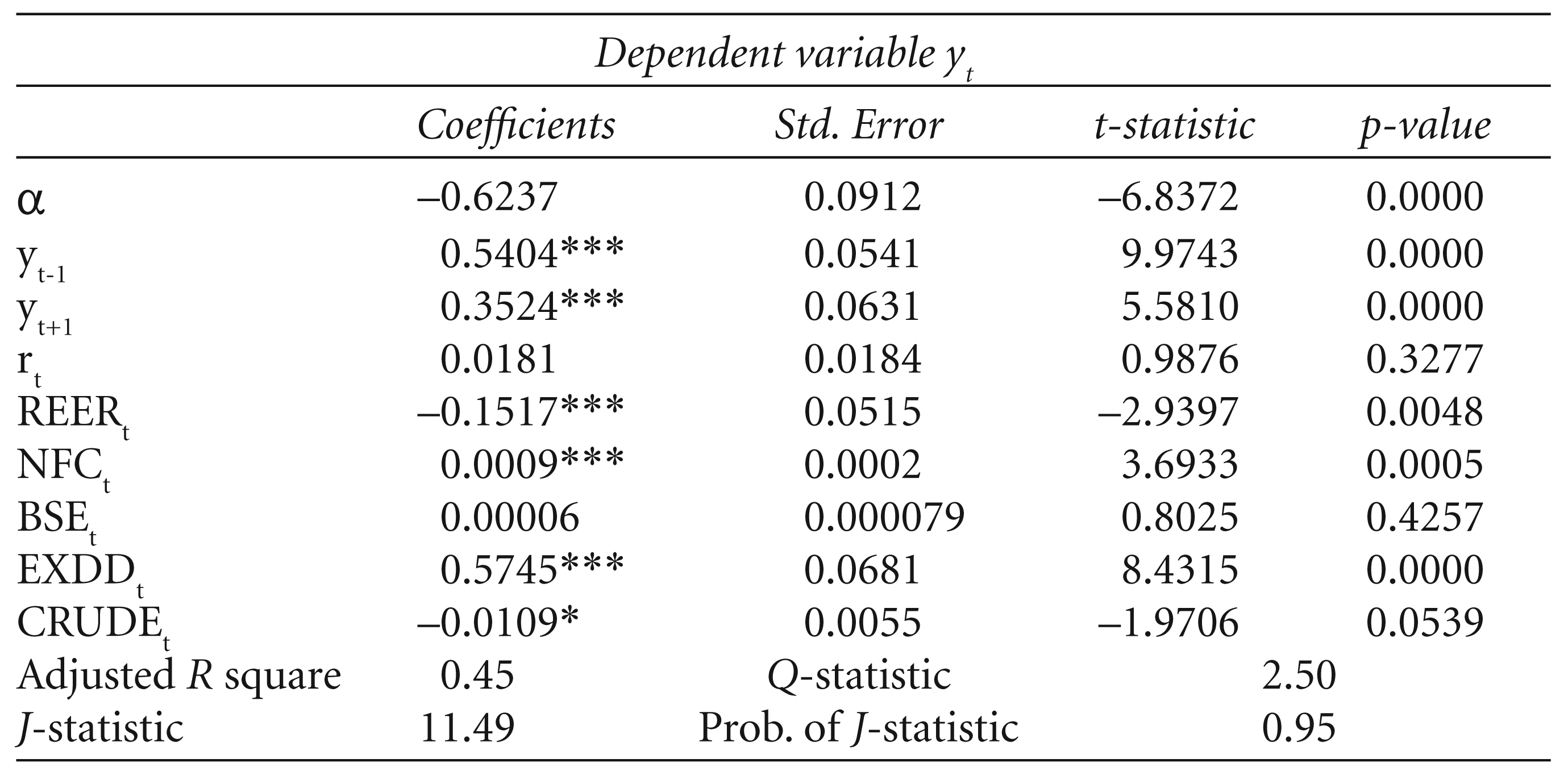
(ii) The Q-statistic denotes the Box-Ljung test statistic for residual autocorrelation.
(iii) The J-statistic and its probability value have been tested for over-identifying restrictions.
Empirical findings on the IS curve using variables in real terms suggest that the backward-looking IS model with real interest rate as the policy variable provides empirically robust results. Even though, in theory, the real interest rate matters for consumption and investment decisions, households appear to respond more to nominal interest rates (Fair, 2002). Hence, to supplement the analysis further and to check for sensitivity of the results to the choice of nominal variables, the present study re-estimates the backward-looking IS equation using all the variables in nominal terms. To estimate the IS model with nominal variables, the study uses non-food credit and world exports in nominal terms. Also, the nominal effective exchange rate (NEER) is used instead of the REER. Tables 5 and 6 provide the estimation results for the backward-looking IS model with nominal variables.
When the IS equation is re-estimated with the nominal interest rate as the policy variable, it is found the nominal interest rate coefficient (–0.20) is of greater magnitude than the real interest rate coefficient (–0.07) in Equation (7). A 1 per cent increase in the nominal interest rate leads to a decrease in the output gap by 0.20 per cent after eight lags. Aggregate demand appears to be more sensitive to the nominal interest rate than to the real interest rate.
OLS Estimates of the Baseline Backward-looking IS Curve (nominal variables)
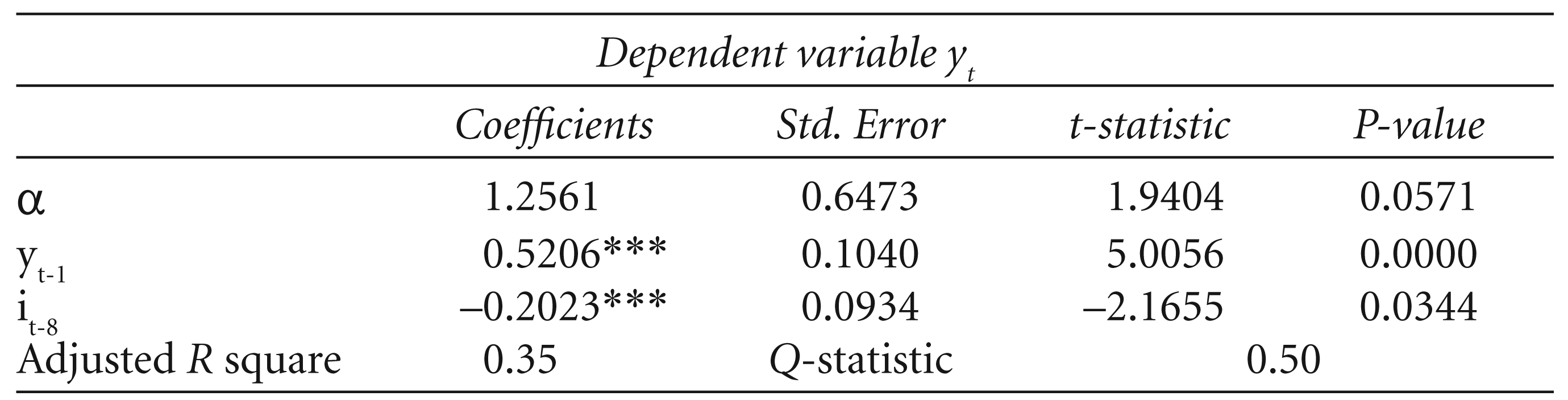
OLS Estimates of the Baseline Backward-looking IS Curve (nominal variables)
(ii) The Q-statistic denotes the Box-Ljung test statistic for residual autocorrelation.
Backward-looking Extended IS Model (nominal variables)
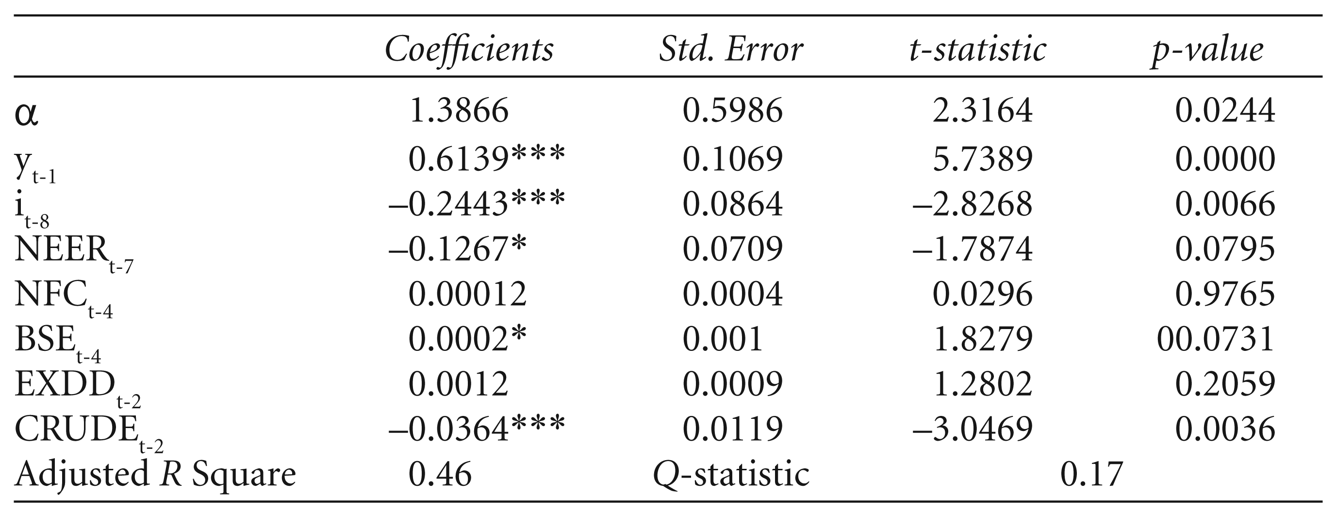
(ii) The Q-statistic denotes the Box-Ljung test statistic for residual autocorrelation.
The baseline backward-looking IS model is extended, as earlier, to account for other variables. As depicted in Table 6, the interest rate coefficient improves to –0.24 when other variables are added to the model. A 1 per cent increase in the interest rate results in a fall in the output gap by 0.24 per cent. Furthermore, an increase in the NEER and crude price index also has a significant and expected impact on the output gap.
The results of the IS estimation using nominal variables align fairly with the estimation results using real variables. The backward-looking IS curve provides robust results in both cases.
The new Keynesian model has become a standard tool for monetary policy analysis. While the baseline theoretical model is purely forward looking, the model that incorporates both forward- and backward-looking elements appears to mirror reality quite well and is also extendable to incorporate country-specific characteristics and open economy considerations. The present study assesses the empirical performance of the new Keynesian IS model by estimating the standard and extended specifications of the backward-looking and hybrid models in India. Drawing from new Keynesian theory, the prime objective of the study is to test the IS equation specified in terms of real variables. Hence, the model has been estimated with variables first in real terms and then, to test the robustness of the results, re-estimated with the variables in nominal terms.
As far as the estimation using real variable is concerned, it is found that the backward-looking models fit the data fairly well compared to the hybrid models. The link between the real policy rate and output gap prevails in both the standard and extended specifications of the backward-looking IS model. Furthermore, the link becomes a bit stronger once the model is extended to account for other variables. Besides the interest rate, the real effective exchange rate, external demand and crude prices have a significant and expected impact on aggregate demand. The results suggest that the standard specification of the IS curve is inadequate to estimate the impact of the interest rate on aggregate demand and, therefore, a broader framework, which accounts for additional variables beside the interest rate maybe required. The hybrid models fail to survive the empirical test, as the interest rate coefficient is insignificant in these models. However, the coefficients on the lead and lag of the output gap are positive and significant. The results from the estimation of the backward-looking IS model using nominal variables broadly aligns with that conducted with real variables.
The empirical robustness of the backward looking IS curve implies that the backward looking behaviour dominates the trajectory of the output. It is generally believed that the monetary policy should be forward looking and should respond to expected inflation and output growth to make the transmission of policy more effective. However, this calls for the forward looking or hybrid nature of the IS curve. The forward looking IS curve necessitates generation of forward looking expectations on various leading indicators in the economy. The task of monetary policy therefore is to track and predict the business cycles and thereby generate forward looking expectations among economic agents. In that sense, the policy has to be more systematic and more rule-based. Furthermore, the monetary policy operates with a lag. When the policy decisions are made in forward looking manner, it is essential to factor in those lags in the transmission process to make the policy more effective. Finally, since the other variables besides the interest rate also have an impact on the aggregate demand, the monetary policy should look into these variables carefully in deciding the policy stance.
Footnotes
Appendix
The Unit Root Test
| Variable | Tests statistic | ||
| ADF test | PP test | KPSS test | |
| Output gap | –4.2782*** | –4.26367*** | 0.1129 |
| Nominal interest rate | –5.3758*** | –2.6929* | 0.4006 |
| real interest rate | –3.0942*** | –2.6892* | 0.6667** |
| ΔREER | –5.87*** | –8.2260*** | 0.0701 |
| ΔReal world exports | –3.87** | –6.3639*** | 0.0447 |
| ΔCRUD | –5.9016*** | –5.7996*** | 0.1903 |
| ΔBSE Sensex | –5.6477*** | –5.2815*** | 0.1026 |
| ΔNFC (Real) | –3.1943** | –5.2535*** | 0.3048 |
| ΔNEER | –3.6935*** | –7.5395*** | 0.1263 |
| ΔNFC (nominal) | –5.1342*** | –16.5687*** | 0.0105 |
| ΔWorld exports (nominal) | –4.6218*** | –7.6310*** | 0.1008 |
(ii) The null hypothesis is of non-stationarity in the case of the ADF and PP tests, and stationarity in the case of the KPSS test.
The additional variables used in the model:
REER = Real effective exchange rate of Indian rupee against the dollar (Trade weighted-36 currencies).
EXDD = External demand proxied by the real world exports.
CRUD = International crude oil price index, NFC (nominal) = Non-food credit.
NFC (real) = Non-food credit deflated using CPI.
BSE = Bombay Stock Exchange Sensex.
NEER = Nominal effective exchange rate (Trade weighted-36 currencies).
Acknowledgements
The authors thank the anonymous referee whose comments helped improve the article significantly.