



Abstract
Though an accumulating body of work has analysed monetary policy transmission in India, there are few studies examining the asymmetric aspect of the transmission. Against this backdrop, segregating the interest rate setting process captured by a Taylor rule type into unanticipated and anticipated components, this article analyses the asymmetric effects of monetary policy on aggregate demand and its components, and inflation in India using quarterly data from 1996–97Q1 to 2013–14Q3. It finds that unanticipated hikes and cuts in the policy rate have a symmetric impact on aggregate demand, but differentially impact the components. While the impacts on investment are negative and symmetric, they are asymmetric on private consumption, with only an unanticipated cut in policy rate having a significant negative impact. Government consumption is unaffected by monetary policy shocks. The impact of unanticipated interest rate changes on inflation is negative and symmetric. Anticipated policy rate changes also have a negative impact on aggregate demand and its components, except for government consumption, but between certain levels, such changes are ineffective, indicating a neutral impact. Anticipated policy rate changes have a negative impact on inflation at all levels.
Introduction
In the literature, various alternative channels of monetary policy transmission have been emphasised, such as the interest rate channel (Taylor, 1995), credit channel (Bernanke & Gertler, 1995), asset prices channel (Meltzer, 1995) and exchange rate channel (Obstfeld & Rogoff, 1995), though these are not entirely mutually exclusive. The interest rate channel works with changes in the policy rate affecting real long-term interest rates in the same direction under the assumption of short-run sticky prices, which in turn influence aggregate demand. The credit channel of transmission assumes importance when banks play a significant role in financial intermediation and there is asymmetry in access to credit between categories of borrowers. Monetary policy easing/tightening by increasing/decreasing deposits could induce higher/lower credit disbursal and impacts aggregate demand. It is also possible that monetary policy, by altering the equity prices of firms and their net worth, can increase bank credit, as there could be fewer concerns for adverse selection of borrowers by banks. The asset price channel would work when a change in monetary policy alters the valuation of equity, which induces a change in household consumption through the associated wealth effect. The same change in monetary policy could alter equity prices and the market value of firms vis-à-vis the replacement cost of capital (Tobin’s ‘q’) and influence the investment activity of firms. Transmission through the exchange rate takes place when, under a flexible exchange rate, a change in monetary policy affects the exchange rate through the resulting interest rate differentials with foreign countries and affects aggregate demand via net exports.
In this context, recent years have seen a number of studies analysing different channels of monetary policy transmission in India (e.g., Aleem, 2010; Al–Mashat, 2003; Bhaumik, Dang & Kutan, 2010; Bhoi et al., 2016; Kapur & Behera, 2012; Khundrakpam, 2013; Khundrakpam & Jain, 2012; Pandit & Vashisht, 2011; Patra & Kapur, 2010; Singh & Kalirajan, 2007). The broad consensus emerging from these is that monetary policy in India works with a lag of about two to three quarters on output and about three to four quarters on inflation, with the impact persisting for 8–12 quarters. Among the channels of transmission, the interest rate channel is found to be the strongest. However, the underlying assumption in all of them is that the impact of monetary policy is symmetric between positive and negative monetary policy shocks. Further, no distinction has been made between anticipated and unanticipated monetary policy changes, though it is debated that it is only the latter which can impact aggregate demand.
Economic theories have emphasised that monetary policy could have an asymmetric impact on the economy. There are at least two main strands of theories explaining the asymmetric impact of monetary policy. First is the credit- rationing hypothesis wherein agents in credit-markets face credit constraints due to information asymmetry. These constraints become more binding during a recessionary phase than an expansionary phase of the business cycle. Thus, policy actions will be more effective when implemented in recessionary situations, as an increase in the cost of capital and tighter liquidity conditions will lead to a decline in investment demand (Bernanke & Gertler, 1989; Gertler, 1988). The other theory is founded on asymmetry in price flexibility in terms of downward stickiness. Due to this downward inflexibility of prices, a fall in aggregate demand due to a contractionary monetary policy leads to a reduction in real output only. In contrast, a rise in aggregate demand due to an expansionary monetary policy moderates the increase in real output due to the accompanying price rise. Thus, a contractionary monetary policy has a stronger impact on real output than an expansionary monetary policy (Ball & Mankiw, 1994; Tsiddon, 1993).
Several studies have empirically examined the asymmetric impact of unanticipated monetary policy shocks on output and inflation for different countries. Many of them support the view that a contractionary monetary policy is more effective than an expansionary monetary policy, including Cover (1992), Morgan (1993) and Thoma (1994) for the USA and Karras (1996a, 1996b) for European economies. However, some studies have contested the above findings arguing that the asymmetric effects of money supply on real output is largely influenced by inflation regimes (Rhee & Rich, 1995; Shen, 2000). Other studies even argue that the above hypothesis either does not hold or that the opposite in fact holds. Rhee (1995) finds that in Korea, there is little empirical support for inflation responding more to positive monetary shocks than negative shocks. And in the case of Australia, Bodman (2006) provides contrary evidence that while an unanticipated expansionary monetary policy raises GDP growth rate significantly, unanticipated monetary policy tightening appears to have no effect.
What about the impact of anticipated monetary policy? Macro rational expectations economists have questioned the traditional view that anticipated monetary policy is effective. They hypothesise that only unanticipated monetary policy can impact the real economy. However, some studies (e.g., Boschen & Grossman, 1981; Mishkin, 1982) have empirically verified that anticipated monetary policy is as effective as unanticipated monetary policy when long lags of output and unemployment are included in the estimation. Though anticipated monetary policy can affect the real economy, it is plausible that there exists some threshold level which separates its effectiveness from its ineffectiveness. In the case of Australia, considering the average policy rate over the sample period as the threshold level, Bodman (2006) found that while an interest rate lower than the average contributes to output growth, a rate that is higher than the average has no impact.
For India, barring a recent one (Aye & Gupta, 2012), hardly any study has analysed either the asymmetric impact of unanticipated monetary policy or the impact of anticipated monetary policy on the economy. Even this study, which employs a non-linear Vector Auto Regression (VAR), analysed the asymmetric impact of an unanticipated change in money supply, and not the interest rate, though in the post-liquidity adjustment facility period since the early 2000s, the interest rate has become the main signalling instrument of monetary policy. The study finds that expansionary money supply shocks have a bigger effect on output than contractionary money supply shocks, but the asymmetric effect lasts only for few quarters. On the other hand, negative shocks have a much greater and persistent impact on inflation than positive shocks.
Further, most of the above referred studies have analysed asymmetry at the level of total aggregate demand, though it is highly plausible that the responses could differ between the components depending upon the behaviour of economic agents and the characteristics of an economy. In fact, it has been shown that in several countries, monetary policy affects aggregate demand mainly through its impact on investment (for example, Barran, Coudert and Mojon (1996) for the EU countries; Disyatat and Vongsinsirikul (2003) for Thailand; and Jakab, Varpalotai and Vonnak (2006) for Hungary). For Thailand, the reason is attributed to the heavy reliance of investment on bank credit, which is sensitive to interest rate changes. As for Hungary, both higher interest rates and the slowdown in investment goods inflation led to a higher user cost of capital, which thus dampened investment, while no significant change was detected in consumption and net exports. With regard to the USA and Euro Area, Angeloni, Kashyap, Mojon and Terlizzese (2003) find that the impact of an unexpected monetary tightening is dominated by a drop in private consumption in the former, while the effect on investments was more important in the latter.
Against the above backdrop, this article attempts to examine the following in the Indian context:
Do unanticipated changes in the policy rate impact aggregate demand and its components, and inflation? If so, are the impacts of unanticipated hikes and cuts in the policy rate symmetric? Do anticipated changes in policy rate also impact aggregate demand and its components, and inflation? If so, are there some threshold levels?
The rest of this article is organised as follows. Second section describes the methodology. The empirical estimates and their interpretations are contained in the third section, and concluding remarks are offered in the fourth section.
Methodology
We draw on the literature, but make necessary adaptations. The analyses are carried out first for an unanticipated change in the policy rate and its asymmetric effects and second for an anticipated change in policy rate and its threshold level.
Unanticipated Change in the Policy Rate and its Effects
The method adopted is similar to the two–step Ordinary Least Squares (OLS) approach as in Cover (1992), Morgan (1993), Ravn and Sola (2004) and Florio (2005). However, the interest rate setting process considered here is different from all of the earlier studies. Cover (1992) considered money supply to be the monetary policy instrument. Morgan (1993) modified the money supply process by an interest rate setting process, which was subsequently employed by several others (e.g., Florio, 2005; MacDonald, Mullineux & Sensarma, 2011). The argument was that it is more appropriate to consider interest rate as the monetary policy instrument than money supply for most advanced economies. Studies covering emerging market economies (EMEs) such as Korea, however, use money supply as the monetary policy instrument, but analysed its asymmetric impact on inflation rather than output (e.g., Rhee, 1995).
In our case, interest rate is considered as the main monetary policy instrument since monetary targeting in India was given up by the late 1990s, and the use of the interest rate as the monetary policy instrument has been increasingly emphasised since the implementation of liquidity adjustment facility by around the late 1990s and the beginning of the 2000s. Thus, we proceed in the following manner. First, we define an unanticipated change in the policy rate by the residuals of an estimate defining the interest rate setting process. Second, the residuals are included in the estimates of models for aggregate demand and its components, and inflation to assess the average impact of an unanticipated change in the policy rate. Third, the residuals are segregated into negative and positive components, representing unanticipated loosening and tightening in the policy rate, respectively. And to examine their asymmetric impacts, they are then included in the same models for aggregate demand and its components, and inflation.
As most of the major central banks, including India’s, are found to follow some interest rate rule, the interest rate setting process is defined by some Taylor rule type as

that is, the interest rate (rt) is determined by the inflation gap (π gapt ) and aggregate demand gap (ygapt) from their respective average, and its own lag, implying interest rate smoothing. In Equation (1), ‘rest’, which is the residual, represents the unanticipated change in the policy rate, which can be segregated into positive and negative components, as pos = max [res, 0] and neg = min [res, 0], respectively.
To analyse the overall impact of an unanticipated change in the policy rate, the lags ‘rest’ are included in the models for estimating aggregate demand and its components (yt), expressed as a function of its own lags and the lags of ‘rest’

For analysing the asymmetric impact of positive and negative interest rate shocks, the lags of ‘pos’ and ‘neg’ are included separately in the corresponding equations, written as

The sum of the coefficients of ‘pos’ and ‘neg’, viz.,
To analyse the similar impact on components of aggregate demand, ‘yt’ in Equations (2) and (3) is replaced by the respective components of aggregate demand, viz., investment (I t ), private consumption (PC t ) and government consumption (GC t ). The precise lag length of the autoregressive term would be determined by the statistical significance, with the maximum being set at four, being quarterly data.
A similar exercise is carried out for inflation (π t ) defining it as a function of its own lags, lags of the output gap ‘OGAPt–i’ and: (i) with lags of ‘rest’ for the overall impact; and (ii) with lags of ‘pos’ and ‘neg’ for asymmetric impact, respectively, as


An anticipated change in the policy rate is defined by the fitted values in Equation (1), as they are components that are predictable through the defined policy rate function of the Taylor rule type. Thus, to examine the corresponding impact of an anticipated change in the policy rate, this fitted component, instead of ‘res’, is included in Equations (2) and (4), and its respective variants representing each component of aggregate demand. These average impacts of an anticipated change in the policy rate, however, could vary at different levels. Thus, to examine the existence of such a differential impact at different levels, the anticipated changes in the policy rate are categorised into two, that is, higher than and lower than a threshold level as,

The high and low policy rates are obtained for various assumed threshold levels. We start from a threshold level of 5.0 per cent and raise it by a discrete 25 basis points each time 1 till 8.0 per cent, as there are few observations outside this range. The high and low policy rate series so defined are then included in Equations (2) and (4), with their variants representing the components of aggregate demand. We primarily focus on the behaviour of the sign and statistical significance of the coefficient of the series representing high policy rates at different threshold levels. This follows since the estimated average impact of anticipated changes in the policy rate for the full sample period represents the coefficient of high policy rates for a threshold level corresponding to the lowest policy rate during the sample period. Thus, as we raise the threshold level, if the coefficient of high policy rates becomes statistically indifferent from zero for a certain range of threshold levels, it could be interpreted as the range where anticipated policy rate is ineffective or neutral.
Data and Results
The time period covered is 1996–97Q1 to 2013–14Q3, as continuous data on quarterly GDP at constant market prices, based on the old series, are available only for this period. All the relevant data, viz., the weighted average call rate, wholesale price index (WPI), GDP at constant market prices and its components, were culled from the RBI’s Real Time Handbook of Statistics on Indian Economy. As in Khundrakpam (2013), a weighted call rate—which is the operating target of monetary policy—has been used as the proxy for the policy rate. This is because till the implementation of the repo rate as the single policy rate following the recommendation of Report of the Working Group on Operating Procedure of Monetary Policy (Reserve Bank of India [RBI], 2011) in 2011, the effective policy rate had alternated between the repo and reverse repo rates depending on whether liquidity was in deficit or surplus. Consequently, prior to 2011, it would be incorrect to consider the repo rate alone as the policy rate. On the other hand, the weighted call rate had mostly mirrored the effective policy rate between the repo and reverse repo rates as the liquidity situation changed—the repo rate when liquidity was in deficit and the reverse repo when it was in surplus. Thus, over the sample period, it was considered more prudent to use the weighted call rate as a proxy for the effective policy rate. As for the inflation rate, the WPI has been considered since it is the main price variable the RBI had monitored under its multiple indicator approach to monetary policy during the sample period considered.
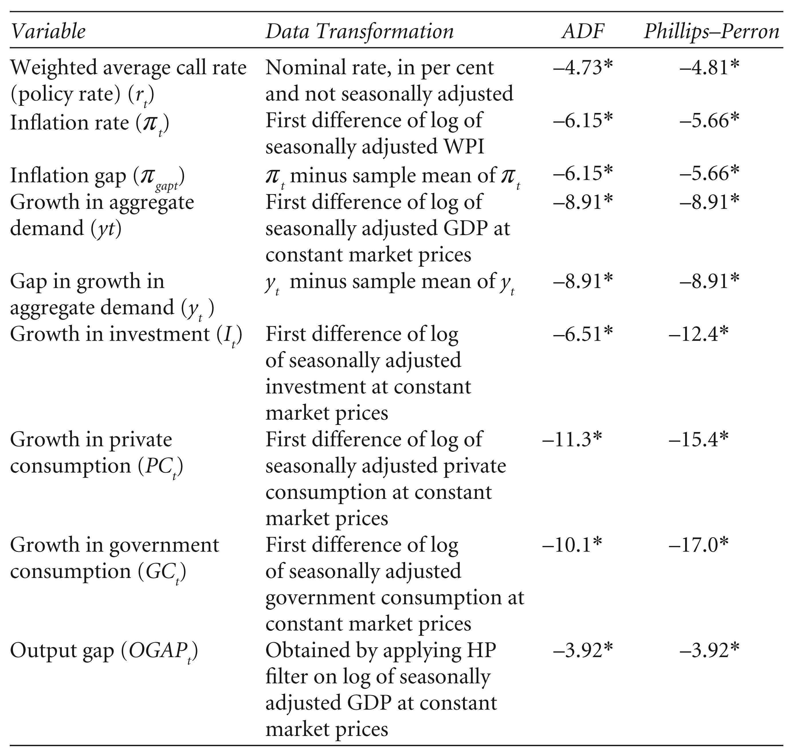
All the variables are in log difference or growth rate form after seasonal adjustment, except for the call rate, and the output gap was obtained by applying an HP filter on the log of the seasonally adjusted GDP at constant market prices. All the variables were found to be stationary by Augmented Dickey–Fuller (ADF) and Phillips–Perron (PP) tests (Table 1). With all the series being stationary, the estimates were carried out using OLS.
Description of Variables
Description of Variables
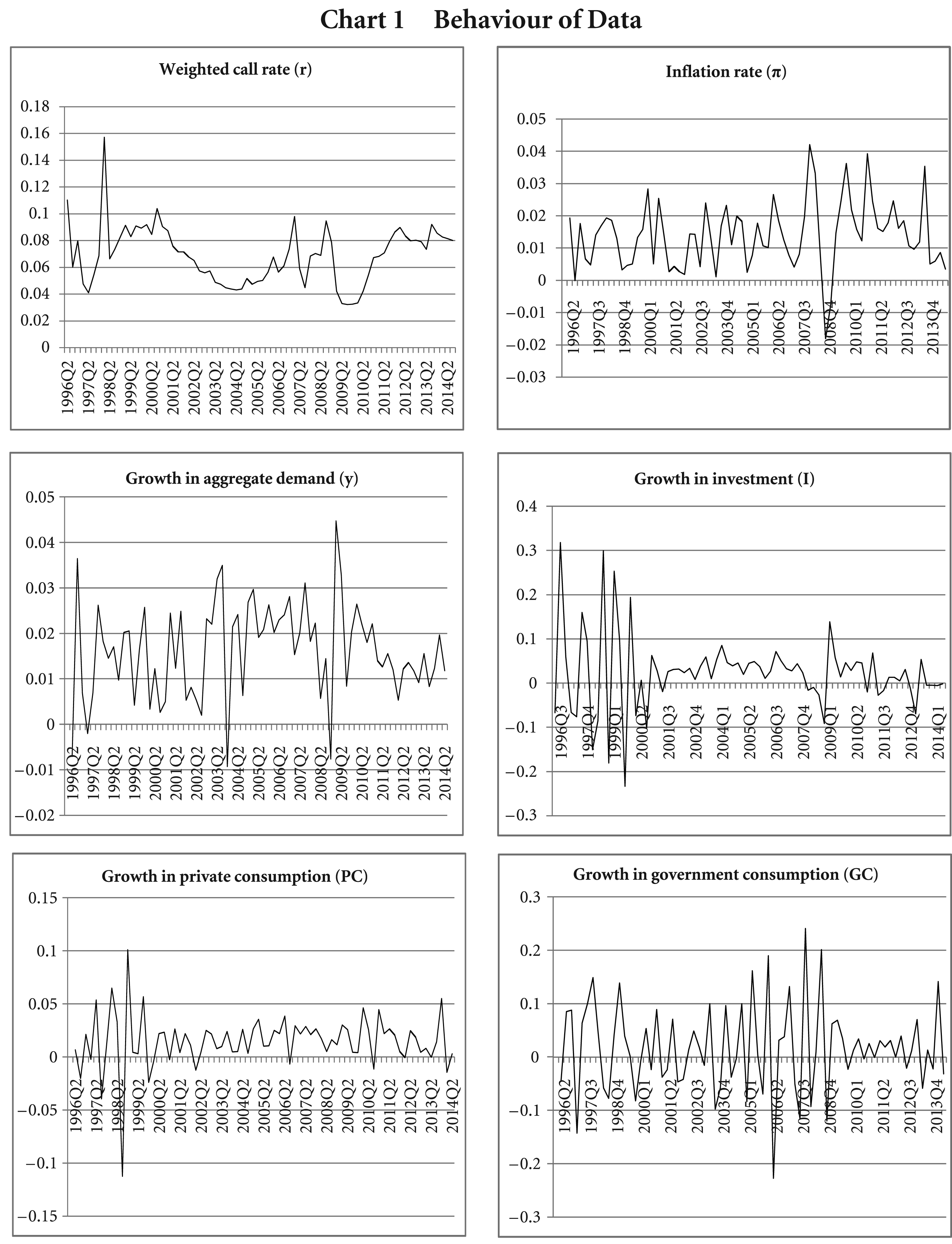
Even though the variables are stationary, as seen in Chart 1, they are quite volatile in nature and there are few outliers in each variable. Since the variables are defined for quarter-on-quarter growth, a positive/negative outlier is often succeeded by a corresponding negative/positive outlier. Thus, in our estimates, the major outliers were controlled through dummies. 2
The estimate for policy rate process is:

R–bar Square = 0.74; Jarque–Bera = 1.41[0.49]; LM–test = 1.27[.27]; BPG = 0.48[.79].
In the above estimate, statistically insignificant lags were progressively dropped from the starting maximum of four lags. Two dummies were included to remove an extreme positive and extreme negative outlier in the estimates in 1998Q1 and 1998Q2, respectively. It can be seen that the policy rate reacts to deviation in inflation with one lag and to output or aggregate demand gap contemporaneously. Further, there is significant policy rate smoothing. As explained above, the unanticipated change in the policy rate is obtained from the residual of this estimate, with a positive and negative residual, respectively, representing unanticipated policy tightening and loosening.
In view of the well-received findings in the literature that monetary policy transmission takes place with variable lags, for each variable we considered four, six and eight lags of unanticipated/anticipated changes in the policy rate. This not only serves as a robustness test, but also enables us to observe lags in the effective transmission of monetary policy shocks. For example, if the sum of the coefficients is statistically significant with four and six lags but not with eight lags, one may interpret it as transmission effectively working only up to six quarters. Similarly, significance with six and eight lags, but not with four lags could imply a transmission lag in monetary policy of about four quarters. In this regard, a common observation from most recent studies on monetary transmission based on VAR models in India is that the effects of a shock to the policy rate on aggregate demand and inflation last for about 8–10 quarters. In the following, the summary of the results along with their analyses are presented, while the details of the diagnostic tests can be found in the appendix Tables A1–A6.
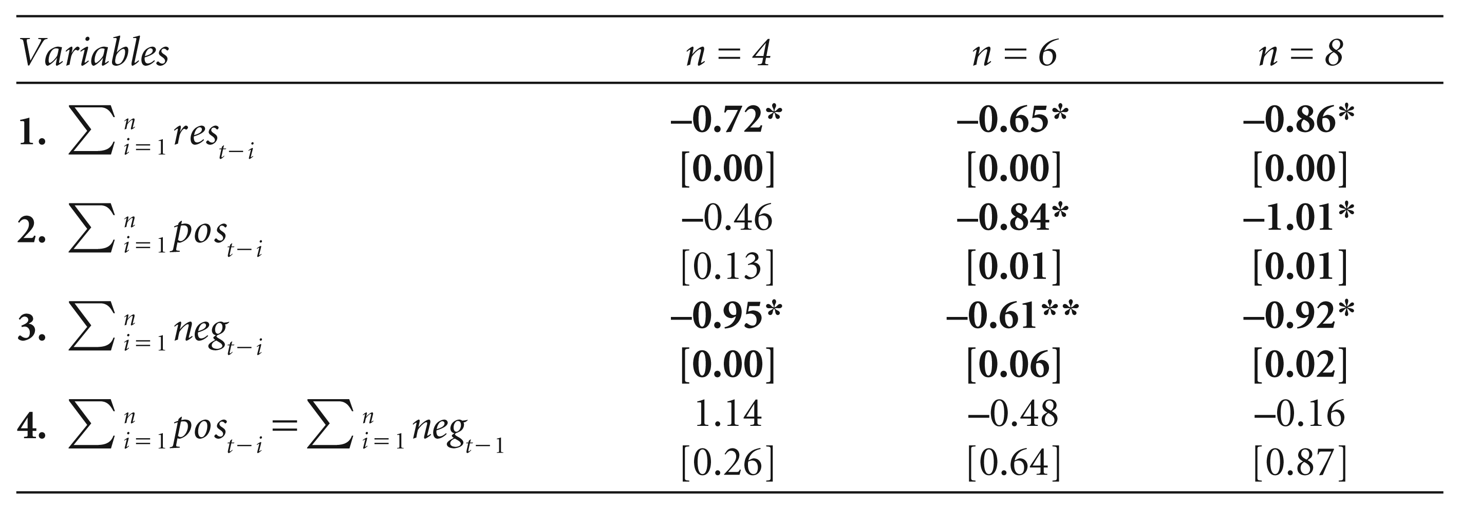
Unanticipated change in the policy rate has a statistically significant cumulative negative impact on aggregate demand growth (row 1, Table 1). This is true for both unanticipated positive and negative policy rate changes, that is, while an unanticipated hike in the policy rate dampens aggregate demand growth (row 2, Table 1), an unanticipated cut in the policy rate enhances it (row 3, Table 1). However, the effective transmission lag of unanticipated policy tightening is longer than that of an unanticipated policy loosening, as the former impact turns statistically significant only after four quarters. Though the impact of tightening appears to be greater than that of loosening after four quarters, the difference is not statistically significant, indicating a symmetric impact or, at best, very weak evidence of asymmetry (row 4, Table 2). Our finding of asymmetry to be, at best, a very weak one is in contrast with that of strong evidence of monetary policy tightening being more effective than loosening for other countries in the literature referred above (e.g., Cover, 1992; Karras, 1996a).
Impact on Investment Growth
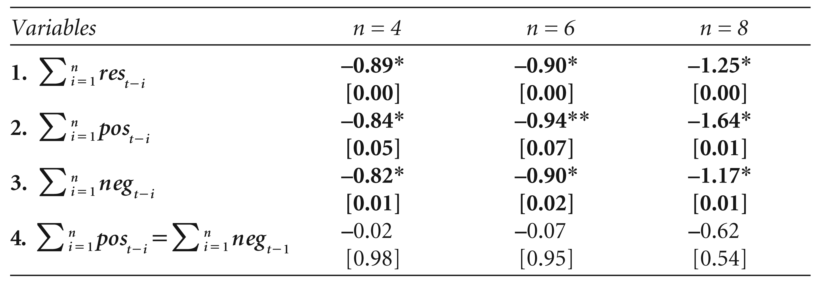
Unanticipated change in the policy rate has a significant cumulative negative impact on real investment growth (row 1, Table 3), with both unanticipated tightening and loosening having a negative impact. In other words, while an unanticipated hike in the policy rate reduces investment growth (row 2, Table 3), an unanticipated cut in the interest rate induces investment growth (row 3, Table 3). However, the transmission lasts longer for an unanticipated hike than for an unanticipated cut in the policy rate, as the magnitude tends to be larger for the former than the latter at longer lags, though they are not statistically different (row 4, Table 3). Thus, the evidence of monetary policy tightening being more effective than monetary policy loosening on investment growth is, again at best, very weak in India. However, that the impact on of unanticipated change in policy rate investment growth is significant is in agreement with the results of other countries (e.g., Disyatat & Vongsinsirikul, 2003; Jakab, Varpalotai & Vonnak, 2006).
Impact of Unanticipated Change in Policy Rate on Aggregate Demand Growth
Impact of Unanticipated Change in Policy Rate on Aggregate Demand Growth
With regard to the overall impact of unanticipated change in the policy rate on private consumption growth, the cumulative negative impact is statistically significant only after four quarters (row 1, Table 4), and that too only for a negative shock (or an unanticipated cut in the policy rate) (row 3, Table 4), and indicates an asymmetric impact (row 4, Table 4). Thus, the interesting inference could be that while an unanticipated cut in the policy rate induces private consumption growth with a lag of about four quarters, an unanticipated hike in the policy rate is not effective in dampening private consumption growth. This is in contrast to the majority of findings in the literature with respect to total aggregate demand.
Impact of Unanticipated Change in Policy Rate on Investment Growth

Impact of Unanticipated Change in Policy Rate on Investment Growth
Impact of Unanticipated Change in Policy Rate on Private Consumption Growth

Unanticipated change in the policy rate on average has no significant negative impact on government consumption growth (row 1, Table 5). However, when we segregate the impacts for positive and negative unanticipated policy rate changes, the former tends to exhibit the perverse impact of increasing government consumption growth (row 2, Table 5), while the latter reduces it (row 3, Table 5), though both are not statistically significant. Consequently, the asymmetric impacts of unanticipated hikes and cuts in the policy rate on government consumption growth become evident by about six quarters (row 4, Table 5). In other words, monetary policy has little impact on government consumption growth in India. This could follow from a large part of government consumption being committed expenditures, while the government has a soft budget constraint to finance them through borrowings which are less sensitive to interest rates.
Impact of Unanticipated Change in Policy Rate on Government Consumption Growth

Impact of Unanticipated Change in Policy Rate on Government Consumption Growth
As with aggregate demand, unanticipated changes in the policy rate have a significant cumulative negative impact on inflation, and the impact gets stronger as the number of lags increase from four to eight, indicating that the impact lasts for more than eight quarters (row 1, Table 6). Both unanticipated positive and negative changes in the policy rate have a negative impact on inflation (rows 2 and 3, Table 6). Though the impact appears to be slightly greater for tightening (positive) than loosening (negative), the difference is not statistically significant (row 4, Table 6). In other words, there is no significant difference between the inflation-reducing impact of unanticipated monetary policy tightening and the inflation-increasing impact of unanticipated monetary policy loosening. This is in line with the finding of Rhee (1995) for Korea when linearity in asymmetry-that is, the transmission of monetary shocks is invariant to the level of average inflation-is assumed, as in our case.
Impact of Unanticipated Change in Policy Rate on Inflation
Impact of Unanticipated Change in Policy Rate on Inflation
Anticipated change in the policy rate also has a significant cumulative negative impact on aggregate demand growth lasting for more than eight quarters. Among its components, the cumulative negative impact lasts more than eight quarters on investment growth and private consumption growth, while there is no significant impact on government consumption growth. In the case of private consumption growth, the transmission lags of anticipated changes in the policy rate are shorter than those of unanticipated changes, which, as estimated above, are more than four quarters. Regarding inflation, an anticipated change in the policy rate, similar to an unanticipated change, has a significant negative cumulative impact on inflation lasting for more than eight quarters (Table 7).
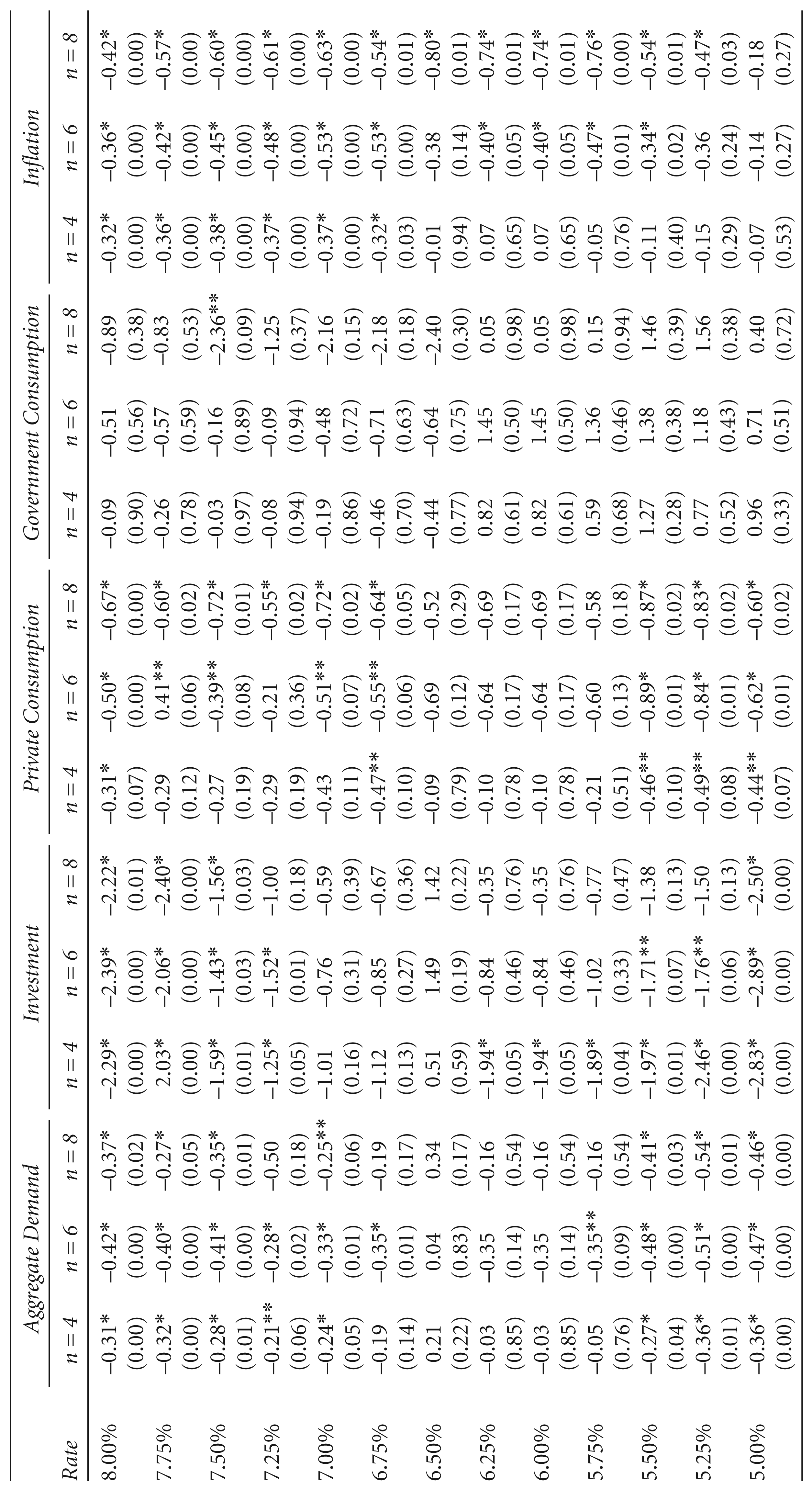
As for the threshold level of anticipated change in the policy rate, considering all the three models, it is seen that policy rate changes between 5.75 and 6.75 per cent have no statistically significant negative impact on aggregate demand growth, while outside this range the impacts are negative. In other words, anticipated policy rate changes could be neutral to aggregate demand growth when they are in the range of 5.75–6.75 per cent. In the case of investment growth, this range is higher by 50 basis points at 6.25–7.25 per cent, while for private consumption growth, the range is slightly wider at 5.5–6.75 per cent. With regard to government consumption growth, anticipated change in the policy rate has a neutral impact at all levels. Interestingly, however, at the lower levels, the impact tends to be perverse (positive impact), but turns negative at the higher levels, though not statistically significant. Regarding inflation, an anticipated change in the policy rate has a negative impact when it is above 5.0 per cent, indicating its non-neutrality at all levels (Table 8).
Anticipated Change in Policy Rate and Its Effects
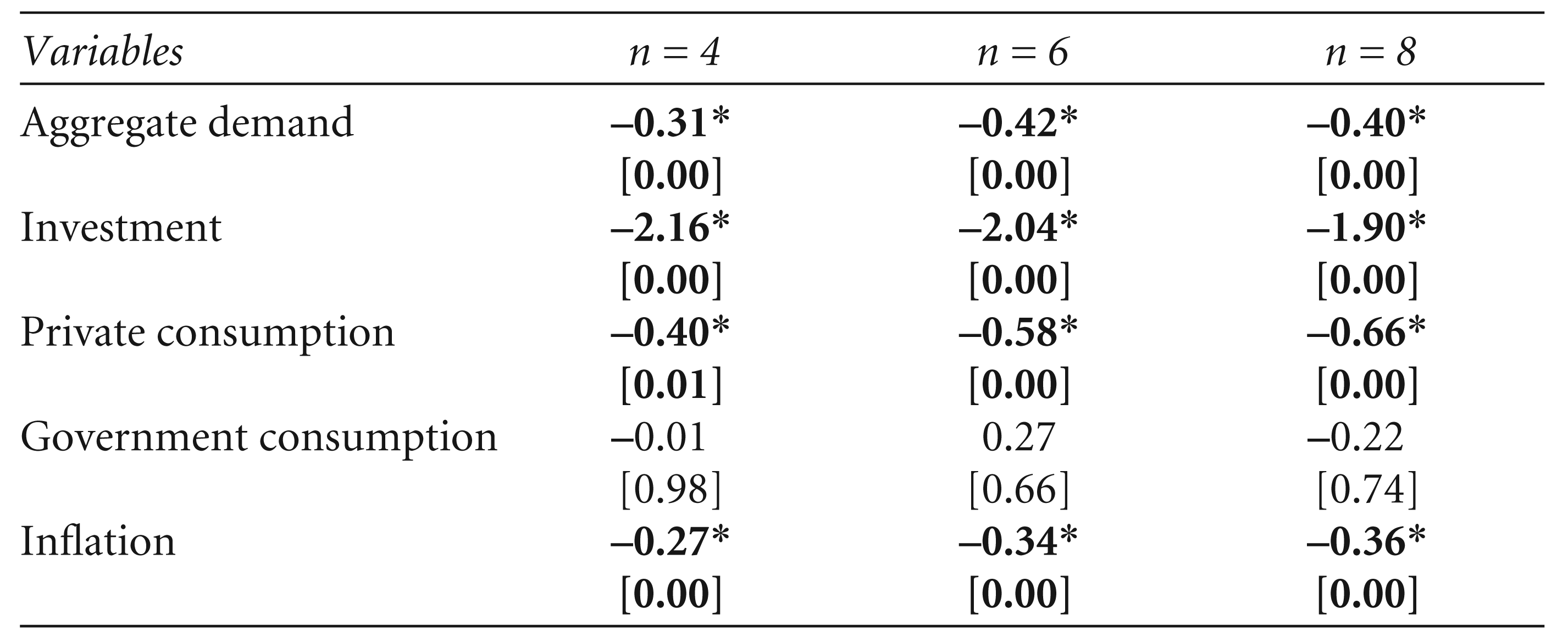
Anticipated Change in Policy Rate and Its Effects
Threshold Levels of Anticipated Change in Policy Rate
Several studies analysing monetary policy transmission in India have shown its effectiveness through the operation of most of the traditional channels, with the interest rate channel being the most effective. However, these studies have, either implicitly or explicitly, assumed symmetric impacts from tight and easy monetary policy. Economic theories, however, emphasise that tight and easy monetary policy could have asymmetric impacts on the economy. Unlike for several other countries, there is hardly any study analysing this aspect of asymmetric transmission of monetary policy, particularly through the interest rate, for India. Further, the analyses of monetary policy transmission have not clearly distinguished between unanticipated and anticipated changes in monetary policy, though in the literature, the effectiveness of the latter has been debated since the emergence of the rational expectations theory. Moreover, the analyses in the Indian context have been largely confined to total aggregate demand, though different components of aggregate demand could differentially respond to monetary policy impulses. Thus, this article was an attempt to fill this gap using quarterly data from 1996–97Q1 to 2013–14Q3.
It finds that unanticipated hikes and cuts in policy rate have a symmetric impact on aggregate demand growth lasting for more than eight quarters. However, they have differential impacts on its various components. While the negative impact is symmetric and faster on real investment growth, the transmission to private consumption growth is not only slower but asymmetric–while unanticipated cuts in the policy rate induce private consumption growth, unanticipated hikes do not curtail private consumption growth. On the other hand, government consumption growth is unaffected by an unanticipated change in the policy rate, and perversely a hike in policy rate tends to increase it. With regard to inflation, unanticipated hikes and cuts in the policy rate have a symmetric impact lasting over eight quarters.
Anticipated policy rate changes also have a negative impact on aggregate demand growth and its components, except for government consumption growth. This finding may be expected given the observation that an increasing number of central banks conduct monetary policy by following some form of policy rule, that is, much of the interest setting may be anticipated/expected, and that monetary policy is potent in the short-run. However, anticipated policy rate change is found to be ineffective or neutral at certain levels. These neutral levels are higher for investment growth than for private consumption growth. On inflation, however, anticipated policy rate changes are found to be non-neutral at all levels.
A few inferences with policy implications may be drawn from these findings. First, unanticipated monetary policy tightening is effective only in reducing investment growth, and none of the other components of aggregate demand, implying that countering short-run heating of the economy through monetary policy shocks could have long-term growth implications, as the brunt is likely to be borne by investment growth. But this policy constraint would not be present during the downturn of a business cycle, as unanticipated monetary policy easing would induce both investment and private consumption growth. Second, in the upturn of a business cycle, anticipated monetary policy changes may be more prudent than monetary policy shocks, as the former would dampen both investment and private consumption growth, while latter would dampen only investment growth.
Third, in an increasingly transparent monetary policymaking environment under an inflation targeting framework, thus, anticipated monetary policy changes by economic agents could be better than unanticipated ones. Fourth, it would be important to recognise the range where anticipated policy rate changes are ineffective or neutral to various components of aggregate demand, which is higher for investment than private consumption, as that would enable recognising the component of aggregate demand that is likely to be most impacted by anticipated monetary policy changes. Fifth, that the effectiveness of monetary policy in the short-run to control aggregate demand growth through investment and private consumption, and therefore, inflation, could be negated by the neutral or even perverse impact on government consumption would highlight the importance of monetary and fiscal policy coordination in India. A caveat to these findings could be, as pointed out in the literature, ignoring the influence of inflation regimes in our analyses, which forms the agenda for future investigation.
Footnotes
Appendix
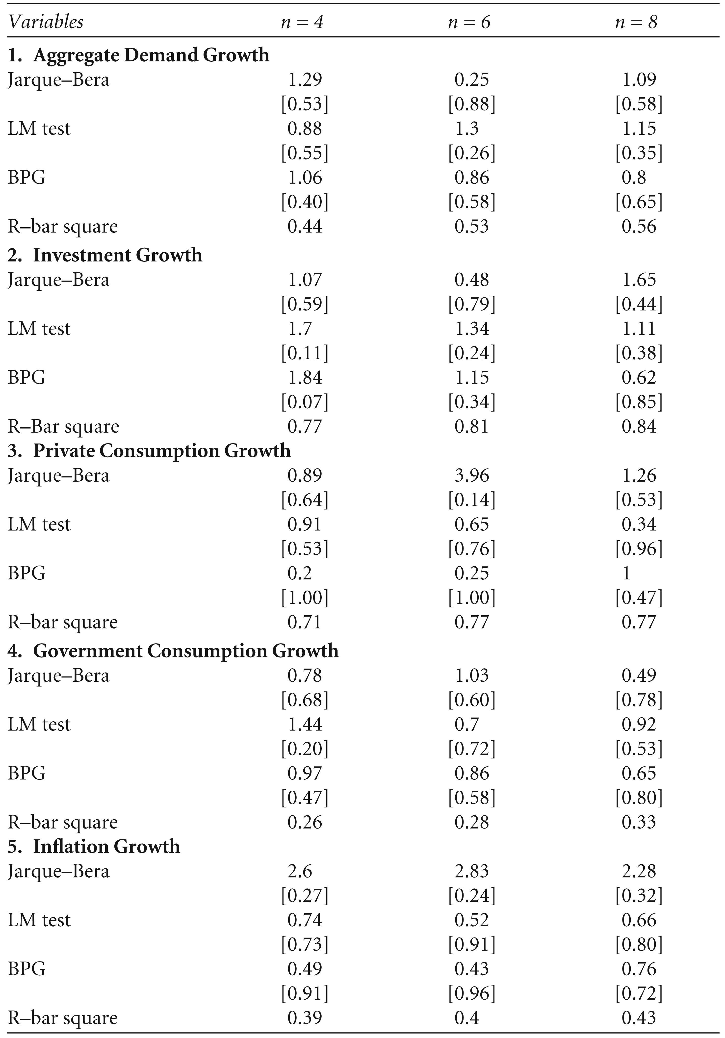
Diagnostics Tests of Anticipated Change in Policy Rate
| Variables | n = 4 | n = 6 | n = 8 |
|
|
|||
| Jarque–Bera | 1.29 | 0.25 | 1.09 |
| [0.53] | [0.88] | [0.58] | |
| LM test | 0.88 | 1.3 | 1.15 |
| [0.55] | [0.26] | [0.35] | |
| BPG | 1.06 | 0.86 | 0.8 |
| [0.40] | [0.58] | [0.65] | |
| R–bar square | 0.44 | 0.53 | 0.56 |
|
|
|||
| Jarque–Bera | 1.07 | 0.48 | 1.65 |
| [0.59] | [0.79] | [0.44] | |
| LM test | 1.7 | 1.34 | 1.11 |
| [0.11] | [0.24] | [0.38] | |
| BPG | 1.84 | 1.15 | 0.62 |
| [0.07] | [0.34] | [0.85] | |
| R–Bar square | 0.77 | 0.81 | 0.84 |
|
|
|||
| Jarque–Bera | 0.89 | 3.96 | 1.26 |
| [0.64] | [0.14] | [0.53] | |
| LM test | 0.91 | 0.65 | 0.34 |
| [0.53] | [0.76] | [0.96] | |
| BPG | 0.2 | 0.25 | 1 |
| [1.00] | [1.00] | [0.47] | |
| R–bar square | 0.71 | 0.77 | 0.77 |
|
|
|||
| Jarque–Bera | 0.78 | 1.03 | 0.49 |
| [0.68] | [0.60] | [0.78] | |
| LM test | 1.44 | 0.7 | 0.92 |
| [0.20] | [0.72] | [0.53] | |
| BPG | 0.97 | 0.86 | 0.65 |
| [0.47] | [0.58] | [0.80] | |
| R–bar square | 0.26 | 0.28 | 0.33 |
|
|
|||
| Jarque–Bera | 2.6 | 2.83 | 2.28 |
| [0.27] | [0.24] | [0.32] | |
| LM test | 0.74 | 0.52 | 0.66 |
| [0.73] | [0.91] | [0.80] | |
| BPG | 0.49 | 0.43 | 0.76 |
| [0.91] | [0.96] | [0.72] | |
| R–bar square | 0.39 | 0.4 | 0.43 |
1. Aggregate demand—(i) 1 for 2004Q1 and 2009Q1 and 0 otherwise and (ii) 1 for 2009Q2 and 0 otherwise.
2. Investment—(i) 1 for 1998Q4 and 1999Q2 and 0 otherwise and (ii) 1 for 1998Q3, 2000Q4 and 2009Q1 and 0 otherwise.
3. Private consumption—(i) 1 for 1997Q4 and 1998Q4 and 0 otherwise for positive outlier.
4. Government consumption—no dummy.
5. Inflation—(i) 1 for 2008Q4 and 0 otherwise and (ii) 1 for 2013Q3 and 0 otherwise.
Acknowledgements
The author thanks the anonymous referee for very useful comments. The views expressed in this article and all errors, whether of omission or commission, are to be attributed to the author only. All the usual disclaimers apply.