Interdependence between Monetary Policy and Stock Liquidity: A Panel VAR Approach

Abstract

This article examines the relationship between monetary policy and individual stock liquidity in an order-driven emerging stock market like India. This study considers stocks listed in National Stock Exchange of India (NSE) and continuously traded from April 2002 to March 2015. Considering the multiple dimensions of liquidity, this study uses five different liquidity proxies to capture the various facets of liquidity such as trading activity, price impact and transaction cost. An array of macroeconomic and firm-specific control variables are used while analysing the liquidity and monetary policy relationship. Econometric methods like panel vector autoregressive (VAR)–Granger causality test, impulse response functions and variance decomposition analysis have been employed to carry out this analysis. The empirical findings suggest that monetary policy significantly Granger-causes stock liquidity, and the expansionary monetary policy characterised by low interest rate and higher money supply is positively associated with individual stock liquidity in India. The impact of monetary policy on liquidity of individual stocks is more prominent during financial crisis. The findings of the present study have certain theoretical as well as practical implications. The market participants in equity market can improve the forecasting of liquidity of their investment portfolio by employing monetary policy along with individual asset’s characteristics. Regulators and policymakers may consider the cross-sectional relationship between stock liquidity and monetary policy as an important source of information for policy formulation and implementation.

JEL Classification: E44, E51, G12

Keywords

Order-driven Emerging stock market Monetary policy Stock liquidity Vector Autoregressive (VAR) model Granger causality Impulse response function Variance decomposition

1. Introduction

A stock is said to be liquid if market participants can buy or sell any amount of it with minimal impact on its price and cost (Amihud, Mendelson, & Pedersen, 2005). Related literature documents that liquidity is critical for hedging and risk management, asset pricing, market efficiency, cost of capital, efficient capital allocation and corporate investment (Acharya & Schaefer, 2006; Amihud & Mendelson, 1989; Borio, 2004; Brunnermeier & Pedersen, 2009; Chordia, Roll, & Subrahmanyam, 2000; Chordia, Sarkar, & Subrahmanyam, 2005; Das & Hanouna, 2009; Wang, 2013). Until recently, the primary focus of market microstructure literature had been to determine the conditions within a stock market that affect liquidity. The seminal work of Chordia et al. (2000), for the first time, emphasises the significance of macroeconomic conditions on determining stock liquidity. The potential impairment caused by the lack of liquidity during the recent financial crisis (2007–2008) has heightened the importance of understanding liquidity and its macroeconomic determinants. In fact, the global financial crisis has been characterised by massive monetary policy interventions by central banks all over the world to infuse liquidity into their financial systems (Trichet, 2010). Therefore, it is worthwhile to examine the relationship between monetary policy and stock liquidity.

Market microstructure literature provides the theoretical linkage between monetary policy and stock liquidity (Hasbrouck, 2007; O’Hara, 1998). Traders provide liquidity to the market, which depends on how economically they can finance their assets. Interestingly, changes in monetary policy measures affect the market rate of interest, which in turn, has an impact on the cost of sourcing finances and, consequently, liquidity in the market (Brunnermeier & Pedersen, 2009; Chordia et al., 2000; Hasbrouck, 2007). The empirical literature on the impact of monetary policy on liquidity has gathered mixed evidence. Goyenko and Ukhov (2009) in the context of the US stock market and Fernandez-Amador, Gächter, Larch and Perter (2013) in the context of the Euro area advocate a strong predictability of monetary policy on stock market liquidity. However, Fujimoto (2003) and Chordia et al. (2005) in the context of the US stock market do not observe predictability of monetary policy on market liquidity. The existing literature has been unable to provide consistent empirical evidence due to variations in sample periods, liquidity and monetary policy proxies and market focus, which makes the comprehensive interpretation of empirical evidence difficult. It thus fails to identify a common consensus on the relationship between monetary policy and stock liquidity and the debate is still unsettled.

From the ongoing discussion on the literature, it is inferred that most studies have been carried out in the context of developed economies and the findings from them are inconclusive. There is a paucity of research in the context of emerging markets, and the only available study, on China (Chu, 2015), reveals asymmetric effects of monetary shocks on stock market liquidity. However, the findings of Chu (2015) do not reveal any insights on the relationship between monetary policy and individual stock liquidity. There is growing unanimity among academic researchers and practitioners that each emerging market economy is unique, with its market structure, regulatory environment and levels of market development (Bekaert & Harvey, 2003). Since financial markets in emerging economies are highly segmented and less mature compared to those in developed countries, it is appealing to understand the monetary policy and liquidity relationship using data from an emerging market which is less correlated with the developed market. As documented by Lo and Mackinlay (1990), an out-of-sample experiment can test whether findings in developed markets should be acknowledged as a worldwide phenomenon.

Against this backdrop, we present the Indian stock market as an ideal candidate for this study. Besides being an order-driven emerging market, it had the following merits: on security listings, it has become the second largest in the world; its size (market capitalisation-to-GDP ratio) has risen from 17.83 per cent in 1991 to 72.4 per cent in 2015 (The World Bank, 2016). It has a turnover ratio of 113.7 per cent compared to developed markets like the USA and the UK which have turnover ratios of 126.5 per cent and 140.5 per cent, respectively (National Stock Exchange of India, 2015). Since the economic reforms initiated since 1991, India’s monetary policy framework has undergone significant changes. It has switched from a monetary-targeting regime (in the mid-1980s) to multiple indicator regimes (1998–1999) and is presently focusing on inflation targeting (Mishra & Mishra, 2012). Concurrently, the focus of monetary policy shifted from direct instruments like selective credit controls and cash reserve ratios to indirect instruments such as repo operations under a liquidity adjustment facility and open market operation (Prabu, Bhattacharyya, & Ray, 2016). The economy too shifted from a largely regulated economy to a market-based one, enlarging the scope for a market-oriented approach for monetary policy formulation. In a market-based financial system, banking and capital market developments are complementary to each other, and hence overall funding conditions are particularly closely tied to fluctuations in the monetary policy environment (Ray & Prabu, 2013). The difference in the structure of the market and policy environment makes it imperative to have out-of-sample empirical evidence from the Indian stock market.

We try to elicit the relationship between monetary policy and an individual stock’s liquidity in a panel vector autoregressive (VAR) framework. We conduct a panel Granger causality test to detect the flow of causality between monetary policy and stock liquidity variables, and carry out impulse response functions (IRFs) analysis to elucidate the response of each stock liquidity measure for a unit positive shock applied to monetary policy variables. Finally, variance decomposition analysis is carried out to determine the percentage of stock liquidity that can be explained by monetary policy.

Our focus on individual stock-level liquidity analysis follows the argument that, while the liquidity of a country’s aggregate equity market is largely determined by macroeconomic factors that are systemic to its economy, unique individual security characteristics determine its relative liquidity (Jun, Marathe, & Shawky, 2003). Considering the multidimensional features of liquidity, we have used five different liquidity proxies to measure trading activity, price impact and transaction cost aspects of liquidity. This approach helps to identify which aspects of liquidity may have greater prominence for a monetary policy impact. Besides, we have used an array of macroeconomic and firm-specific control variables, which have been identified as major determinants of liquidity in the relevant literature. The study finds a strong predictability of monetary policy on stock liquidity, which is consistent with Goyenko and Ukhov (2009) and Fernandez-Amador et al. (2013). To our knowledge, this study could perhaps be the first-ever empirical evidence on monetary policy implications for an individual stock’s liquidity, focussing on pure order-driven market data in emerging markets. The estimated results derived from an emerging order-driven market can be compared with the existing evidence from developed quote-driven markets, to gain more insight on the monetary policy–liquidity relationship.

The rest of the article is organised as follows. Section 2 presents a brief literature review. Section 3 deals with measurement of variables. Section 4 describes data and the preliminary analysis. Section 5 elaborates on the empirical approach. Section 6 discusses the empirical results and, finally, Section 7 concludes.

2. Review of the Literature

Over the past two decades, a large body of literature supports the view that stock market development positively influences economic growth, which depends upon the liquidity creation of stock markets (Atje & Jovanovic, 1993; Haugen & Baker, 1996; Jun et al., 2003; Levine & Zervos, 1998). Liquid markets tend to exhibit characteristics such as tightness or low transaction costs, immediacy or speed of order execution, depth, breadth and resiliency (Sarr & Lybek, 2002). The available literature supports the claim that liquidity impacts financial market prices (Amihud & Mendelson, 1989; Chordia et al., 2000) and illiquidity behaves as a systematic risk factor for describing the time-series and cross-sectional behaviour of expected return (Amihud, 2002; Pastor & Stambaugh, 2003).

The theoretical linkage between monetary policy and market liquidity is embedded in the market microstructure literature. The inventory theory of market microstructure proposes that inventory turnover and the risk of holding inventory affect market liquidity (Hasbrouck, 2007; O’Hara, 1998). This indicates that the cost of financing and the risk of holding stocks are two fundamental attributes that influence the liquidity of a stock. Liquid stocks show the characteristics of low cost of financing and less inventory risk. Interestingly, both the costs associated with financing assets and the risks of holding securities are affected by changes in monetary policy. Thus, monetary policy is expected to affect stock liquidity. The monetary stance of the central bank can affect stock market liquidity by altering the borrowing constraint and fund flow into the stock market (Brunnermeier & Pedersen, 2009; Garcia, 1989).

Brunnermeier and Pedersen (2009) developed a model that establishes a link between an asset’s market liquidity and funding liquidity. The model suggests that market participants having capital constraints find it difficult to meet their margin requirements and, in turn, fail to provide liquidity. Conversely, corrosion of market liquidity increases the cost of the margin, which reduces traders’ funding liquidity. Following these arguments, an expansionary monetary policy is expected to reduce the cost of margin borrowing by traders and to facilitate funding liquidity; the reverse may be expected during a tightening of monetary policy. The existing literature on asset liquidity documents a considerable co-movement of an individual stock’s liquidity, which is known as commonality in liquidity (Chordia et al., 2000; Huberman & Halka, 2001). The observed commonality in liquidity implies that illiquidity is a systematic risk factor and cannot be diversified (Acharya & Pedersen, 2005; Pastor & Stambaugh, 2003). These observations compel us to believe that there may be some underlying economic forces or at least one common factor which concurrently determines the liquidity of all stocks in the market. We assume monetary policy as the suitable macroeconomic candidate to serve the purpose.

There is a dearth of academic literature that empirically examines the predictability of monetary policy on stock liquidity. Early research by Fujimoto (2003) examines the relationship between macroeconomic fundamentals and market liquidity for all stocks listed on the NYSE and AMEX for a sample period from 1965 to 2001. The study approximates monetary policy through non-borrowed reserves and the federal funds rate. The empirical findings suggest an increase in liquidity for a positive innovation in non-borrowed reserves and a decrease in stock liquidity for a hike in the federal funds rate before 1982. This implies that monetary policy considerably influenced stock liquidity during 1965 to 1982. However, for the period ranging from 1983 to 2001, none of the monetary policy variables are found to predict stock liquidity. Similarly, Chordia et al. (2005) investigate the predictability of monetary policy on stock market liquidity for all stocks listed on the NYSE. The study uses the federal fund rate and net-borrowed reserves as measures of monetary policy and finds that monetary policy influences market liquidity only in the crisis period. Soderberg (2008) also derives mixed evidence of predictability of macroeconomic variables on market liquidity for the Scandinavian stock exchanges (the Copenhagen Stock Exchange, Oslo Stock Exchange and Stockholm Stock Exchange). The study concludes that the policy rate predicts market liquidity in the Copenhagen Stock Exchange, broad money growth rate in the Oslo Stock Exchange, and the short-term interest rate and mutual fund flows predict liquidity in the Stockholm Stock Exchange. There is no common determinant which can forecast market liquidity for all the three stock exchanges.

In contrast to the above findings, Goyenko and Ukhov (2009) for a period ranging from 1962 to 2003 obtain a strong evidence for predictability of monetary policy on stock market liquidity for US market (NYSE and AMEX). Their study reveals that an expansionary monetary policy, which is reflected in an increase in non-borrowed reserves and a decrease in the federal fund rate, enhances market liquidity. In a recent study, similar evidence was noted by Fernandez-Amador et al. (2013) in the context of the Euro zone. Their study documents that the expansionary monetary policy decisions taken by the European Central Bank (ECB) enlarge overall stock market liquidity in the German, French and Italian markets. As well, monetary policy significantly influences individual stock level liquidity.

To briefly sum up, the extant review of relevant literature does not find any consensus on whether monetary policy predicts stock liquidity or not, and which monetary policy instrument is better at liquidity predictability. There are also a limited number of empirical studies which have examined the interrelationship between the monetary policy environment and stock liquidity in emerging economies. Since each emerging market is unique, with its own market structure, currency area and market focus, a study on the nexus between monetary policy and stock liquidity may provide some new insights. Further, the Indian stock market, apart from being an order-driven emerging market, has witnessed several reform initiatives in the recent past for the conduct of monetary policy (Aleem, 2010; Prabu et al., 2016). These observations warrant a fresh investigation to ascertain the monetary policy and stock liquidity relation.

3. Variables

Following the review of literature, we choose liquidity, monetary policy and other control variables for this study.

3.1 Liquidity Variables

Liquidity, by its very nature, is difficult to define and even more difficult to estimate because it encompasses a number of transactional properties of markets (Kyle, 1985; Lesmond, 2005). Stock market liquidity has multiple dimensions, such as tightness (the difference between buy and sell price or bid–ask spread), depth (the ability to buy or sell certain quantity of securities without any impact on quoted prices), immediacy (the velocity with which a transaction gets executed) and resiliency, which reflects how quickly prices revert to the previous level after the transaction of a certain quantity of assets (Kyle, 1985; Sarr & Lybek, 2002). Considering these facets of liquidity, we employ five different liquidity proxies to capture attributes such as trading activity, price impact and transaction costs.

Trading activity is an intuitive and indirect measure of an asset’s liquidity. The selection of liquidity proxies with respect to trading activity is motivated by the findings of Amihud and Mendelson (1986), which assert that the liquidity of a stock is an increasing function of trading frequency in equilibrium. That means that investors prefer to hold securities with higher trading frequency to avoid illiquidity risk. Following Fernandez-Amador et al. (2013), we use the turnover rate (TR) and traded value (TV) in rupees as proxies to measure the trading activity of stocks. Considering the importance of trading frequency, Datar, Naik and Radcliffe (1998) introduced TR as an indirect measure of liquidity of an asset, which can be computed as the number of shares traded to the number of shares outstanding. Their study also documents that a higher TR is related to greater liquidity. We also use TV (the product of the number of shares traded with their respective prices) as another variable to measure trading activity. Stocks with higher TVs exhibit greater liquidity (Brennan, Chordia, & Subrahmanyam, 1998; Stoll, 1978).

The price impact dimension of liquidity can be defined as the change in the price of an asset for a unit change in the volume of transaction (i.e., the response of the asset’s price to the flow of orders). We have employed the Amihud (2002) illiquidity measure (ILLIQ) and turnover price impact (TPI) to capture the price impact characteristics of stock liquidity. The ILLIQ measures the response of return from a stock for every rupee change in trading volume (Amihud, 2002). We have chosen this proxy for two reasons. First, it has been widely used as a measure of illiquidity in most recent literature such as Acharya and Pedersen (2005), Fujimoto (2003), Goyenko and Ukhov (2009) and Fernandez-Amador et al. (2013). Second, it is easy to calculate and does not require any sophisticated microstructure data. Apart from these advantages, it has also been considered as a fine measure of price impact among most low-frequency liquidity proxies (Goyenko, Holden, & Trzcinka, 2009; Hasbrouck, 2007; Lesmond, 2005). This ratio also has several advantages over other traditional measures of liquidity. Specifically, it may have a price discovery component, such as future expectation or information about stock price movement that might influence trading activity. Also, it serves as a good empirical proxy for determining liquidity in a cross-sectional study (Korajczyk & Sadka, 2008).

This ratio can be computed as the absolute return from any security ‘i’ (for the month t) (|R_i,d|) with respect to the traded volume (TV_i,d) in rupees, averaged over the number of trading days in that month (D_i).

I L L I Q = 1 / D_{i} \sum_{d = 1}^{D_{i}} \frac{| R_{i, d} |}{T V_{i, d}}

Despite the wide popularity of the ILLIQ measure, it has some key limitations. It always indicates that small size stocks (having low market capitalisation) are more illiquid than large size stocks, as smaller stocks have a lower trading volume, which is the denominator of ILLIQ. This implies that the ILLIQ has a size bias, and the value of the ratio might generate ambiguity in cross-sectional studies. Second, inflationary conditions may also have an impact on this ratio, as trading volumes are measured in monetary units. Also, it does not consider the trading frequency aspect of securities, which is documented as one of the fundamental attributes of stocks liquidity (Datar et al., 1998). Considering these shortcomings, Florakis, Gregoriou and Kostakis (2011) introduced the turnover price impact ratio as a simple and adequate measure of stock liquidity. This ratio can be computed as the absolute return from any security ‘i’ (for the month t) (|R_i,d|) with respect to the turnover rate (TR_i,d), averaged over the number of trading days in that month (D_i).

T P I = 1 / D_{i} \sum_{d = 1}^{D_{i}} \frac{| R_{i, d} |}{T R_{i, d}}

To capture the transaction cost aspect of liquidity, we have employed the high–low spread (HLS) ratio as proposed by Corwin and Schultz (2012). The study reveals that HLS is an effective measure of illiquidity in developed as well as emerging economies like India and Hong Kong. Corwin and Schultz (2012) suggest a high correlation between actual stocks spread and HLS estimates, that is, 0.9 under realistic conditions. In addition, it is very easy to compute and does not require high-frequency market microstructure data (such as the bid price, ask price and so on). The computation of this ratio requires only the daily high price of stocks (which reflects trades initiated by buyers) and daily low price of stocks (which reflects trades initiated by sellers). Thus, the high–low price ratio of a stock on a particular day reflects the daily primary stock volatility and spread (bid–ask spread).

We calculate HLS ratio as follows:

H L S = \frac{2 * (e^{α} - 1)}{1 + e^{α}}

where α can be determined as $α = \frac{\sqrt{(2 * β)} - \sqrt β}{3 - 2 * \sqrt 2} - \sqrt{\frac{γ}{3 - 2 * \sqrt 2}},$ $β = \sum_{i = 0}^{1} \ln (\frac{H_{t + i}^{O}}{L_{t + i}^{O}}), γ = \sum_{i = 0}^{1} \ln (\frac{H_{t, t + i}^{O}}{L_{t, t + i}^{O}})$ , H^O= observed high price of a stock on day i and L^O = observed low price of a stock on day i.

3.2 Monetary Policy Variables

We have approximated the monetary policy of a central bank through monetary aggregates and the interest rate. Taking a cue from Fernandez-Amador et al. (2013), we employ the rolling 12-month reserve money growth rate (RM) as a proxy for the monetary aggregate. We chose reserve money because it is very easily affected by the policy decisions of the monetary authority.

Re s e r v e m o n e y g r o w t h r a t e = \frac{R M_{t} - R M_{t - 12}}{R M_{t - 12}} * 100

It is also evident from extant literature that the interest rate has emerged as a crucial information variable for financial markets (Dhal, 2000). In line with the previous literature, we use the monthly weighted average call money rate (CMR) as a measure of the monetary stance. The change in the CMR reflects the dynamics of the demand and supply of overnight liquidity requirement (similar to the Fed rate for the US and Euro overnight index average for the Euro Central Bank). We are motivated to choose the CMR as an approximation of monetary policy due to its recognition as the operating target of monetary policy by the Reserve Bank of India since late May 2011.

3.3 Other Control Variables

Following existing studies (Chordia et al., 2001; Eisfeldt, 2004; Fernandez-Amador et al., 2013; Goyenko & Ukhov, 2009; Soderberg, 2008), we have used the rolling 12-month growth rate of inflation (IR) and industrial production growth rate (IP) as macroeconomic variables in our study. We have taken into account the effect of market conditions on stock market liquidity (Brunnermeier & Pedersen, 2009; Copeland & Galai, 1983; Hameed, Kang, & Viswanathan, 2010) by including stock returns (RET) and stock volatility (STDV) as market-related control variables in our model. Amihud (2002) argues that the impact of illiquidity shocks on larger firms is less pronounced than the smaller size securities. Following this reasoning, one can also argue that the effect of policy variables (monetary policy) on stock liquidity may differ depending on the size of the firm. Thus, we include firm’s size (SZ) as another firm-specific control variable in the panel model, measuring it as the natural logarithm of the market capitalisation of firms. Considering the possible interdependence of liquidity and cyclical movement in the stock market, following Fernandez-Amador et al. (2013), we incorporate INDEX (i.e., the monthly return of benchmark index of NSE, CNX NIFTY 50) as a variable in our study.

4. Data and Sample Characteristics

The present study takes into consideration all NSE-listed stocks. The sample period spans from April 2002 to March 2015. We choose 2002 as the start for data collection to avoid covering two different trading systems: the Security Exchange Board of India (SEBI) abolished the ‘badla system’ in July 2001 and introduced the rolling settlement cycle (T + 2) to facilitate transparency, efficiency and immediacy. Following Chordia et al. (2005), we set the following criteria to select stocks for our study:

The stock should be present at the beginning and end of the data period, that is, April 2002 and March 2015.

The stock should have been continuously traded throughout the sample period (i.e., April 2002 to March 2015) and disseminated daily trading information, such as its closing price, high price, low price and stock turnover, as we require this information to compute the liquidity measures.

Stocks not actively traded were dropped, which means that a stock having a constant price for more than 1 month is not considered in our sample.

Considering the undue influence of high-priced stocks, we exclude stocks having abnormally high values at the end of any month in a year.

We find that only 510 firms (out of 1,483 firms) meet the above criteria to become our study sample. We have collected the daily high price, low price, opening price, closing price and trading volume for the selected stocks to determine daily returns, volatility and liquidity proxies. Then, the daily measures are averaged to construct a monthly proxy, as most of the macroeconomic variables are available on monthly frequency. The total number of observations for the panel data is 79,560 (156 time-series observations for 510 cross sections). All the stock market-related data have been collected from the Bloomberg database and official website of the NSE; data on macroeconomic fundamentals are obtained from the RBI’s Handbook of Statistics.

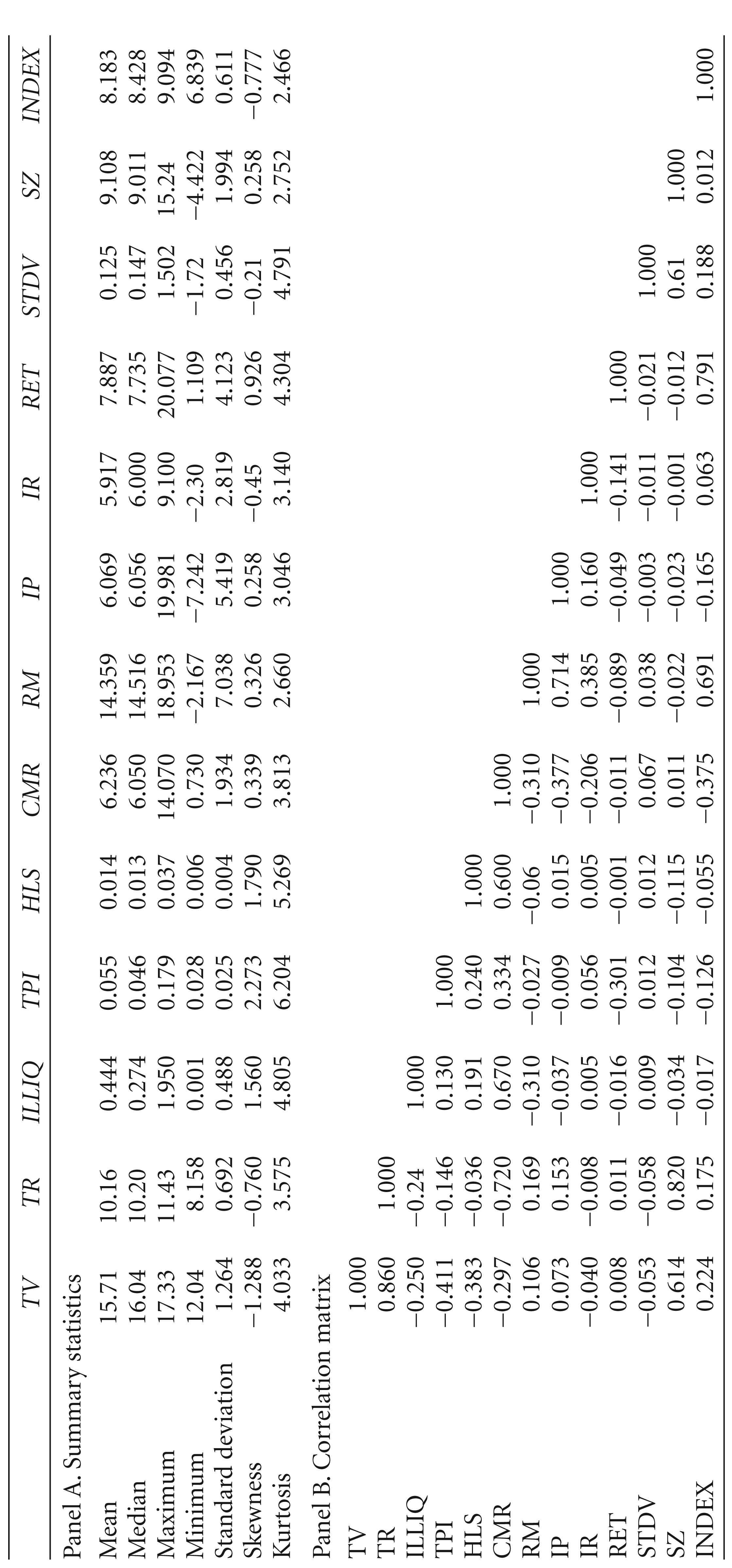
The summary statistics and correlation matrix of liquidity variables (TV, TR, ILLIQ, TPI, HLS), monetary policy variables (CMR, RM) and control variables (IP, IR, STDV, RET, SZ, INDEX) are presented in Table 1. ‘Panel A’ indicates the descriptive statistics and ‘Panel B’ highlights the correlation structure among the employed variables in our model. Some interesting observations emanate from the correlation matrix. It has been found that the liquidity measures (TV and TR) are negatively associated with STDV and have a positive relationship with RET. This indicates that the volatility of stock returns can be perceived as an indicator of illiquidity. Similarly, the bivariate correlation between stock returns and liquidity indicates that returns of a stock are an increasing function of liquidity. We find a negative correlation between the trading activity measures of liquidity (TV and TR) and price impact measures (ILLIQ and TPI). A similar relationship has also been observed between the measures of trading activity and transaction costs (HLS), indicating that higher trading activity translates into increased liquidity of stocks; however, the increase in the cost of transactions or a price impact reduces the liquidity of financial assets. Our correlation analysis reflects a small degree of association among liquidity measures. This may be due to the fact that liquidity is multidimensional in nature and the employed liquidity proxies measure the different aspects of liquidity and do not represent the same sets of information. We observe a positive association between money supply (RM) and trading activity, and a negative correlation between trading activity and the interest rate (CMR). Besides, the correlation between the HLS, ILLIQ and TPI with the RM is found to be negative. We infer from these observations that monetary policy may influence stock market liquidity and vice versa.

Table 1
Summary Statistics and Correlation Matrix

TV TR ILLIQ TPI HLS CMR RM IP IR RET STDV SZ INDEX

Panel A. Summary statistics

Mean 15.71 10.16 0.444 0.055 0.014 6.236 14.359 6.069 5.917 7.887 0.125 9.108 8.183

Median 16.04 10.20 0.274 0.046 0.013 6.050 14.516 6.056 6.000 7.735 0.147 9.011 8.428

Maximum 17.33 11.43 1.950 0.179 0.037 14.070 18.953 19.981 9.100 20.077 1.502 15.24 9.094

Minimum 12.04 8.158 0.001 0.028 0.006 0.730 −2.167 −7.242 −2.30 1.109 −1.72 −4.422 6.839

Standard deviation 1.264 0.692 0.488 0.025 0.004 1.934 7.038 5.419 2.819 4.123 0.456 1.994 0.611

Skewness −1.288 −0.760 1.560 2.273 1.790 0.339 0.326 0.258 −0.45 0.926 −0.21 0.258 −0.777

Kurtosis 4.033 3.575 4.805 6.204 5.269 3.813 2.660 3.046 3.140 4.304 4.791 2.752 2.466

Panel B. Correlation matrix

TV 1.000

TR 0.860 1.000

ILLIQ −0.250 −0.24 1.000

TPI −0.411 −0.146 0.130 1.000

HLS −0.383 −0.036 0.191 0.240 1.000

CMR −0.297 −0.720 0.670 0.334 0.600 1.000

RM 0.106 0.169 −0.310 −0.027 −0.06 −0.310 1.000

IP 0.073 0.153 −0.037 −0.009 0.015 −0.377 0.714 1.000

IR −0.040 −0.008 0.005 0.056 0.005 −0.206 0.385 0.160 1.000

RET 0.008 0.011 −0.016 −0.301 −0.001 −0.011 −0.089 −0.049 −0.141 1.000

STDV −0.053 −0.058 0.009 0.012 0.012 0.067 0.038 −0.003 −0.011 −0.021 1.000

SZ 0.614 0.820 −0.034 −0.104 −0.115 0.011 −0.022 −0.023 −0.001 −0.012 0.61 1.000

INDEX 0.224 0.175 −0.017 −0.126 −0.055 −0.375 0.691 −0.165 0.063 0.791 0.188 0.012 1.000

	TV	TR	ILLIQ	TPI	HLS	CMR	RM	IP	IR	RET	STDV	SZ	INDEX
Panel A. Summary statistics
Mean	15.71	10.16	0.444	0.055	0.014	6.236	14.359	6.069	5.917	7.887	0.125	9.108	8.183
Median	16.04	10.20	0.274	0.046	0.013	6.050	14.516	6.056	6.000	7.735	0.147	9.011	8.428
Maximum	17.33	11.43	1.950	0.179	0.037	14.070	18.953	19.981	9.100	20.077	1.502	15.24	9.094
Minimum	12.04	8.158	0.001	0.028	0.006	0.730	−2.167	−7.242	−2.30	1.109	−1.72	−4.422	6.839
Standard deviation	1.264	0.692	0.488	0.025	0.004	1.934	7.038	5.419	2.819	4.123	0.456	1.994	0.611
Skewness	−1.288	−0.760	1.560	2.273	1.790	0.339	0.326	0.258	−0.45	0.926	−0.21	0.258	−0.777
Kurtosis	4.033	3.575	4.805	6.204	5.269	3.813	2.660	3.046	3.140	4.304	4.791	2.752	2.466
Panel B. Correlation matrix
TV	1.000
TR	0.860	1.000
ILLIQ	−0.250	−0.24	1.000
TPI	−0.411	−0.146	0.130	1.000
HLS	−0.383	−0.036	0.191	0.240	1.000
CMR	−0.297	−0.720	0.670	0.334	0.600	1.000
RM	0.106	0.169	−0.310	−0.027	−0.06	−0.310	1.000
IP	0.073	0.153	−0.037	−0.009	0.015	−0.377	0.714	1.000
IR	−0.040	−0.008	0.005	0.056	0.005	−0.206	0.385	0.160	1.000
RET	0.008	0.011	−0.016	−0.301	−0.001	−0.011	−0.089	−0.049	−0.141	1.000
STDV	−0.053	−0.058	0.009	0.012	0.012	0.067	0.038	−0.003	−0.011	−0.021	1.000
SZ	0.614	0.820	−0.034	−0.104	−0.115	0.011	−0.022	−0.023	−0.001	−0.012	0.61	1.000
INDEX	0.224	0.175	−0.017	−0.126	−0.055	−0.375	0.691	−0.165	0.063	0.791	0.188	0.012	1.000

Source: Authors’ own computation.

Notes: This table represents the descriptive statistics and correlation matrix of the liquidity variables, that is, traded value (TV), turnover rate (TR), illiquidity ratio (ILLIQ), turnover price impact (TPI), high–low spread (HLS); monetary policy variables, that is, call money rate (CMR), reserve money growth rate (RM); macroeconomic control variables, that is, industrial production growth rate (IP), inflation rate (IR); and other control variables, that is, monthly stock return (RET), monthly stock standard deviation (STDV), firm’s size (SZ) and return from the CNX NIFTY 50 index (INDEX). Sample period consists of 156 monthly observations across 510 cross sections (79,560) from April 2002 till March 2015.

5. Empirical Approach

Although the pertinent literature has partially explained the univariate relationship among macroeconomic fundamentals, market variables and stock market liquidity, there are good reasons to expect a bidirectional relationship among them. For example, investors demand higher expected return for holding illiquid stock in equilibrium (Amihud & Mendelson, 1986). However, it has also been argued that the return from a stock signals future trading behaviour, which in turn, affects stock liquidity. In the same direction, Garcia (1989) highlights the importance of monetary policy decisions in infusing liquidity into the market, particularly during crisis periods, as a minimum level of liquidity is required for smooth functioning of financial markets. Hence, stock market liquidity may be a function of macroeconomic variables. On the other hand, Næs, Skjeltorp and Ødegaard (2011) posit that stock market liquidity is a leading indicator of the real economy and its desertion in the financial market is a precursor to a crisis or distress in the real economy. Based on these arguments, we expect an endogenous relationship between stock liquidity and indicators of the real economy.

Given the arguments, to investigate the relationship between monetary policy and stock liquidity, we employ a panel VAR model as it is suitable for analysing the cause–effect relationship in a multivariate framework and it assumes that all the variables are endogenous. We consider the panel data model, which combines the properties of both time-series and cross-sectional data which allows individual heterogeneity to vary across firms (Love & Zicchino, 2006). The traditional Granger causality (Granger, 1969) model is used to know the direction causality of time-series variables. Consistent with Holtz-Eakin, Newey and Rosen (1988), we specify the panel Granger causality model as follows:

X_{j, t} = a_{j} + \sum^{​} ​ a_{1 j t} * X_{j, t - i} + \sum^{​} ​ b_{1 j t} * Y_{j, t - 1} + u_{j, t}

(1)

Y_{j, t} = a_{j} + \sum^{​} ​ b_{2 j t} * Y_{j, t - i} + \sum^{​} ​ a_{2 j t} * X_{j, t - 1} + v_{j, t}

(2)

where the X vector represents monthly stock liquidity measures at time ‘t – i’ across firms ‘j’; the Y vector represents the monthly measures of monetary policy and control variables (macroeconomic as well as market variables) at time ‘t – i’ across firms ‘j’; ‘i’ represents the minimum lag length; a_1jt and a_2jt are coefficients of the lagged value of the X vector; b_1jt and b_2jt are coefficients of the lagged value of the Y vector; u_j,t and v_j,t are the error terms of Equations (1) and (2), respectively; and a_j represents the panel fixed effects, which changes across firms, however, time invariant. This model examines whether stock liquidity and monetary policy are linked together, and whether any spontaneous change in monetary policy influences stock liquidity. To choose the optimal lag length m, we have employed the Akaike information criterion (AIC) and the Schwarz information criterion (SIC). Although the two criteria show different lag lengths, we have chosen the smaller one to retain the maximum number of degrees of freedom. Before estimating this model, we have carried out the unit roots tests developed by Levin–Lin–Chu (LLC) (Levin, Lin, & Chu, 2002) and Im–Pesaran–Shin (IPS) (Im, Pesaran, & Shin, 2003). Both LLC and IPS are widely used and consistent with the augmented Dickey–Fuller (ADF) (1981) approach. The LLC test assumes homogeneity in the dynamics of the autoregressive coefficients for all panel values, while the IPS test assumes heterogeneity in these dynamics. Therefore, the IPS test is known also as the heterogeneous panel unit root test.

The IRFs are meant to elucidate the dynamic reaction of one variable to the innovations in another variable in the system, while keeping all other shocks equal to zero. However, since the actual variance–covariance matrix of the errors is unlikely to be diagonal, to isolate shocks to one of the variables in the system it is necessary to decompose the residuals in such a way that they become orthogonal. The usual convention is to adopt a particular ordering and allocate any correlation between the residuals of any two elements to the variable that comes first in the ordering. Following Goyenko and Ukhov (2009), we have ordered the variables in such a way that they influence each other. For the IRFs, it is necessary to estimate the confidence intervals. Since the matrix of IRFs is constructed from the estimated VAR coefficients, their standard errors need to be taken into account. We calculate standard errors of the IRFs and generate confidence intervals with Monte Carlo simulations. Finally, we conduct variance decompositions to know the per cent variation in one variable that is explained by the shock to another variable, accumulated overtime. The Equations (2) and (3) are estimated following the procedure laid down by Abrigo and Love (2016).

6. Discussion of the Results

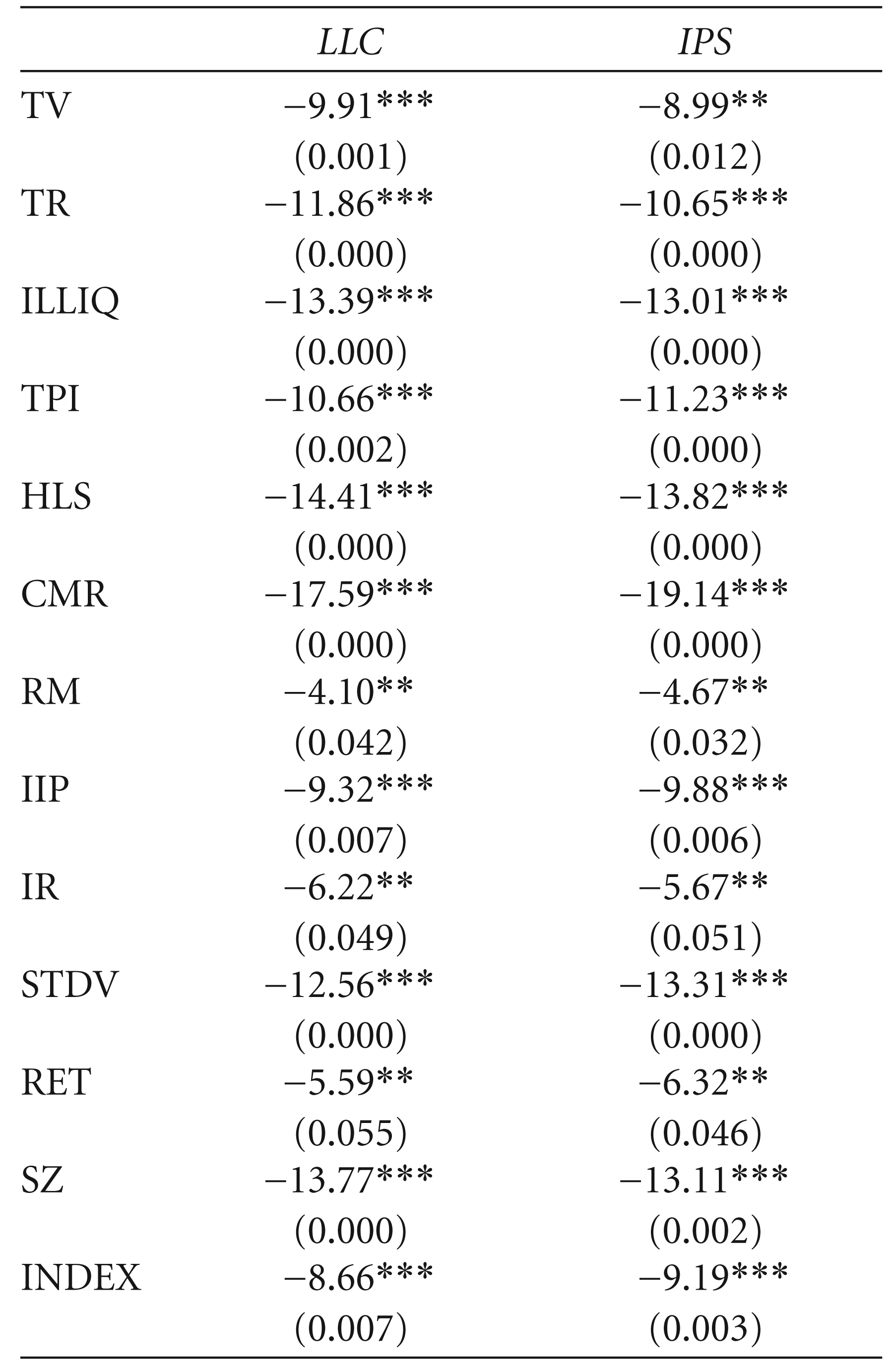
This section deals with the empirical findings of the panel VAR–Granger causality test, IRFs and variance decomposition, to ascertain the relationship between monetary policy and stock liquidity. First, we report the unit root tests results, followed by the Granger causality test, IRFs and variance decomposition. The unit root test statistics (LLC and IPS) are reported in Table 2. The unit root tests reveal that the null hypothesis of the unit root is rejected for all the liquidity measures, macroeconomic variables and firm-specific variables at the first difference. Since most of the liquidity variables are stationary at the first difference, we have reported the unit root test statistics at the first difference only. Also, we have used the variables in their first difference in our model. The use of variables at first difference is also motivated by Wooldridge (2002), which asserts that this reduces the problem of serial correlation and trending of data to a larger extent.

Table 2
Panel Unit Root Test Statistics

LLC IPS

TV −9.91*
(0.001) −8.99
(0.012)

TR −11.86*
(0.000) −10.65*
(0.000)

ILLIQ −13.39*
(0.000) −13.01*
(0.000)

TPI −10.66*
(0.002) −11.23*
(0.000)

HLS −14.41*
(0.000) −13.82*
(0.000)

CMR −17.59*
(0.000) −19.14*
(0.000)

RM −4.10
(0.042) −4.67
(0.032)

IIP −9.32*
(0.007) −9.88*
(0.006)

IR −6.22
(0.049) −5.67
(0.051)

STDV −12.56*
(0.000) −13.31*
(0.000)

RET −5.59
(0.055) −6.32
(0.046)

SZ −13.77*
(0.000) −13.11*
(0.002)

INDEX −8.66*
(0.007) −9.19*
(0.003)

	LLC	IPS
TV	−9.91*** (0.001)	−8.99** (0.012)
TR	−11.86*** (0.000)	−10.65*** (0.000)
ILLIQ	−13.39*** (0.000)	−13.01*** (0.000)
TPI	−10.66*** (0.002)	−11.23*** (0.000)
HLS	−14.41*** (0.000)	−13.82*** (0.000)
CMR	−17.59*** (0.000)	−19.14*** (0.000)
RM	−4.10** (0.042)	−4.67** (0.032)
IIP	−9.32*** (0.007)	−9.88*** (0.006)
IR	−6.22** (0.049)	−5.67** (0.051)
STDV	−12.56*** (0.000)	−13.31*** (0.000)
RET	−5.59** (0.055)	−6.32** (0.046)
SZ	−13.77*** (0.000)	−13.11*** (0.002)
INDEX	−8.66*** (0.007)	−9.19*** (0.003)

Source: Authors’ own computation.

Notes: This table presents the Levin–Lin–Chu (LLC) and Im–Pesaran–Shin (IPS) panel unit root tests. *** and ** indicate the significance at the 1% and 5% levels, respectively.

We employ a panel VAR model to analyse the relationship between stock liquidity and the monetary stance. In order to interpret the estimated model, we report the panel Granger causality test, IRFs and variance decomposition analysis. In this case, we estimated the VAR model for all the five stock market liquidity measures and two monetary policy variables. This entails a total of 10 different VAR estimates, each of which allows for 42 Granger causality tests. We have reported the Granger causality tests between five liquidity proxies and two monetary policy variables. We test the null hypothesis that the lagged value of the endogenous variable (either monetary policy variables or stock liquidity) does not Granger-cause the dependent variable (again, stock liquidity or macroeconomic variables). Table 3 reports the χ² statistics and p-values of pairwise Granger causality tests between endogenous VAR variables.

Table 3

Panel VAR–Granger Causality Tests for Monetary Policy and Stock Liquidity

Panel A. Granger causality tests: monetary policy and stock market liquidity (H₀: Monetary policy does not Granger-cause stock liquidity)
Variables	TV	TR	ILLIQ	TPI	HLS
CMR	65.30*** (0.00)	22.85*** (0.00)	6.93** (0.05)	1.45 (0.55)	4.63* (0.09)
RM	28.77*** (0.00)	1.12 (0.39)	1.29 (0.27)	7.55** (0.04)	1.73 (0.23)
Panel B. Granger causality tests: liquidity variables and monetary policy (H₀: Stock liquidity does not Granger-cause monetary policy)
Variables	CMR		RM
TV	0.77 (0.64)		0.89 (0.35)
TR	0.15 (0.87)		0.31 (0.58)
ILLIQ	3.09* (0.08)		1.37 (0.19)
TPI	0.19 (0.84)		0.58 (0.47)
HLS	2.98 (0.09)		0.88 (0.36)

Source: Authors’ own computation.

Notes: This table presents the χ² statistics of pairwise panel Granger causality tests between endogenous variables. The figures in parentheses represent p-values. The sample period consists of 156 monthly observations across 510 firms from April 2002 to March 2015. ***, ** and * indicate significance at the 1%, 5% and 10% levels, respectively.

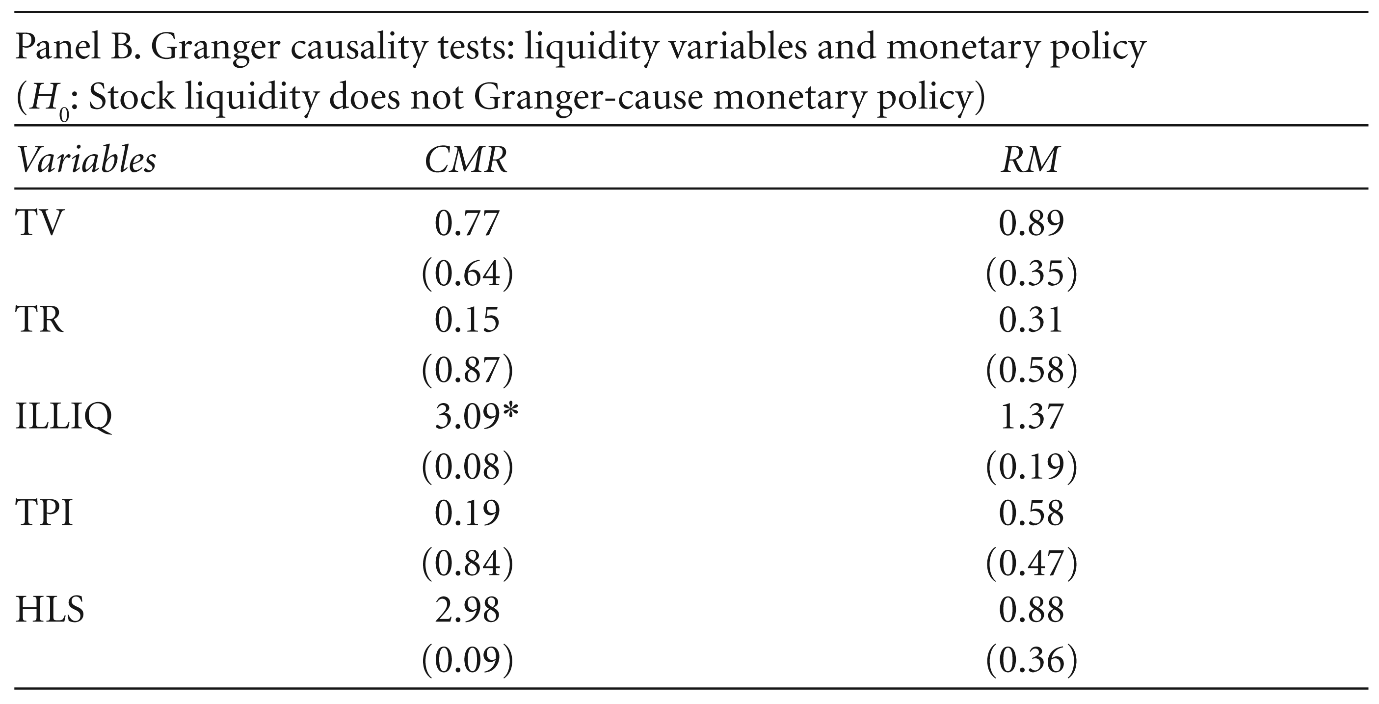
Panel A in Table 3 indicates that the monetary policy variables (CMR and RM) are informative in predicting stock market liquidity. We find that a change in CMR significantly Granger-causes some trading activity, price impact and transaction cost measures, though not all. To check the consistency of our findings, we re-examine the relationship between monetary policy and stock liquidity by employing RM and obtain the similar findings. Interestingly, Panel B of Table 3 documents very little evidence of the flow of causality from stock liquidity to monetary policy. This forfeits the notion of the existence of a bidirectional causality between monetary policy and stock liquidity and firmly establishes the unidirectional relationship between them. Overall, the results present sufficient evidence in favour of monetary policy causing stock liquidity.

To understand the dynamic interactions among the variables in the model, we conduct IRF analysis. We primarily aim to trace the dynamic reaction of stock liquidity for every unit standard deviation innovation in monetary policy variables. Figure 1 demonstrates the response of stock liquidity to a unit standard deviation change in the CMR, traced forward over a period of 10 months. A positive shock to the CMR reduces TV and stock TR. This implies a declining trend in market trading activity. In the same way, from Figure 2, we have noticed a positive influence of money supply on stock liquidity. This analysis shows that an expansionary monetary policy, which is characterised by a lowering of the interest rate or increasing of the money supply, strengthens stock liquidity, while a tightening of monetary policy is associated with a decline in stock liquidity. Our findings from the IRFs are consistent with the findings of Goyenko and Ukhov (2009) and Fernandez-Amador et al. (2013).

Figure 1

Source: Authors’ own computation.

Figure 2

Source: Authors’ own computation.

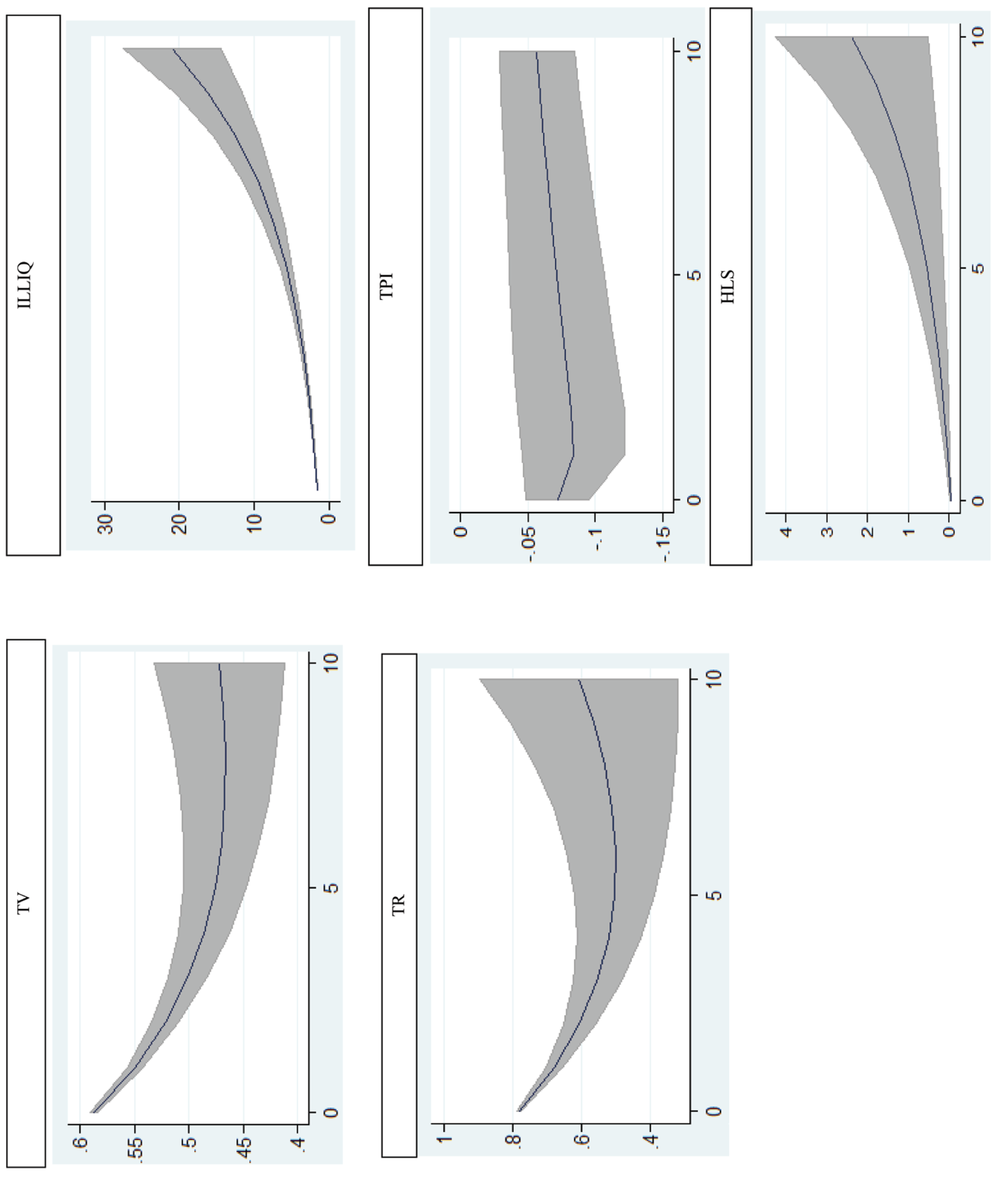
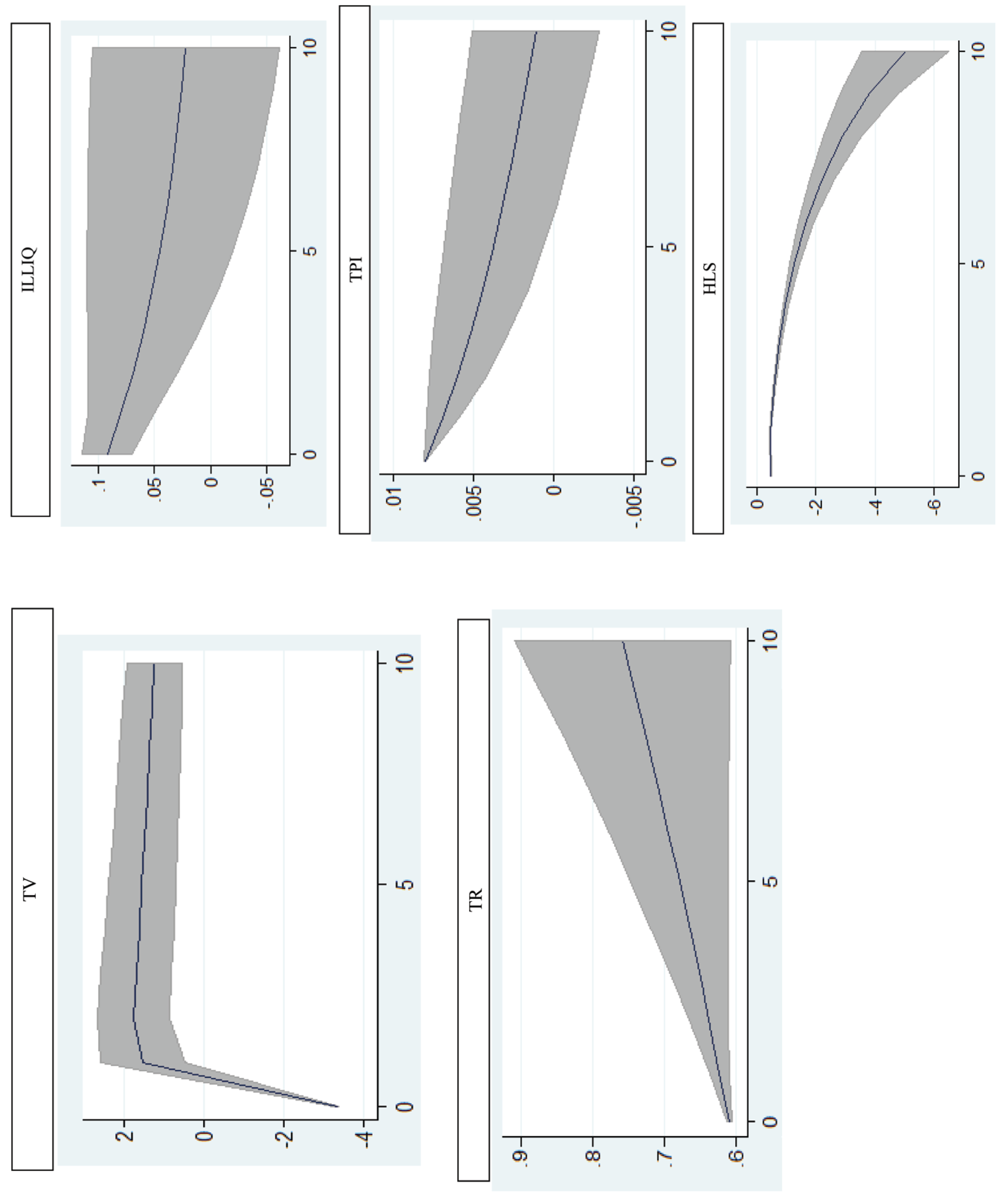
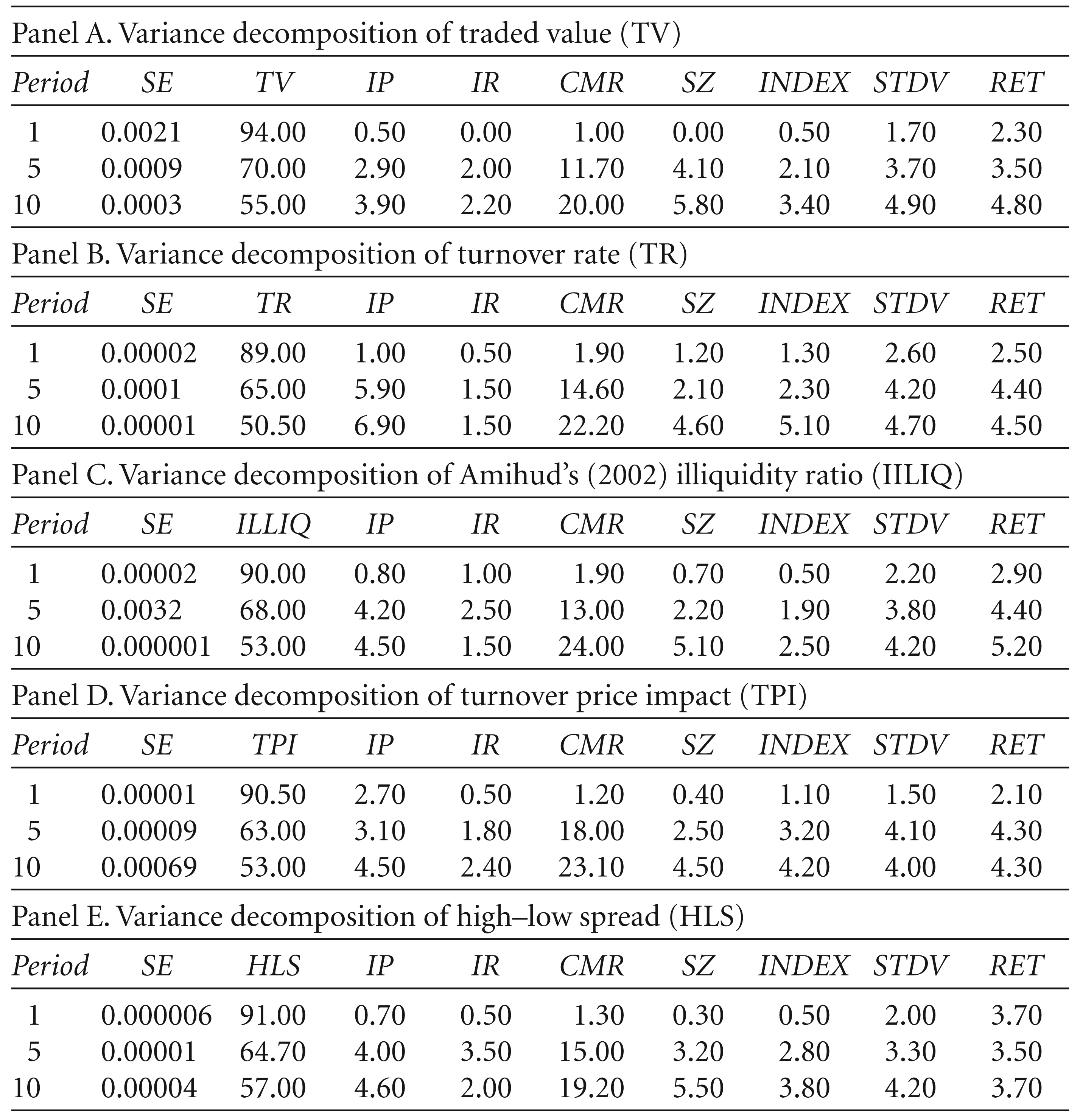
Table 4 reports the variance decomposition of liquidity variables when monetary policy is approximated by the CMR. We find little evidence of the immediate effect of monetary policy on stock liquidity; however, the impact is found to be prominent after 5 months. This implies that monetary policy influences liquidity with some lag. Besides monetary policy, we have also noticed that the industrial production growth rate, stock returns, stock volatility and firm’s size are crucial in explaining variation in liquidity. We have also conducted the variance decomposition of the liquidity variables when monetary policy is proxied by the RM. The estimated results, reported in Table 5, further confirm the significant role of monetary policy in determining stock liquidity. The results are similar to those reported in Table 4, where the monetary policy is through the CMR.

Table 4

Variance Decomposition of Liquidity Variables for the CMR

Panel A. Variance decomposition of traded value (TV)
Period	SE	TV	IP	IR	CMR	SZ	INDEX	STDV	RET
1	0.0021	94.00	0.50	0.00	1.00	0.00	0.50	1.70	2.30
5	0.0009	70.00	2.90	2.00	11.70	4.10	2.10	3.70	3.50
10	0.0003	55.00	3.90	2.20	20.00	5.80	3.40	4.90	4.80
Panel B. Variance decomposition of turnover rate (TR)
Period	SE	TR	IP	IR	CMR	SZ	INDEX	STDV	RET
1	0.00002	89.00	1.00	0.50	1.90	1.20	1.30	2.60	2.50
5	0.0001	65.00	5.90	1.50	14.60	2.10	2.30	4.20	4.40
10	0.00001	50.50	6.90	1.50	22.20	4.60	5.10	4.70	4.50
Panel C. Variance decomposition of Amihud’s (2002) illiquidity ratio (IILIQ)
Period	SE	ILLIQ	IP	IR	CMR	SZ	INDEX	STDV	RET
1	0.00002	90.00	0.80	1.00	1.90	0.70	0.50	2.20	2.90
5	0.0032	68.00	4.20	2.50	13.00	2.20	1.90	3.80	4.40
10	0.000001	53.00	4.50	1.50	24.00	5.10	2.50	4.20	5.20
Panel D. Variance decomposition of turnover price impact (TPI)
Period	SE	TPI	IP	IR	CMR	SZ	INDEX	STDV	RET
1	0.00001	90.50	2.70	0.50	1.20	0.40	1.10	1.50	2.10
5	0.00009	63.00	3.10	1.80	18.00	2.50	3.20	4.10	4.30
10	0.00069	53.00	4.50	2.40	23.10	4.50	4.20	4.00	4.30
Panel E. Variance decomposition of high–low spread (HLS)
Period	SE	HLS	IP	IR	CMR	SZ	INDEX	STDV	RET
1	0.000006	91.00	0.70	0.50	1.30	0.30	0.50	2.00	3.70
5	0.00001	64.70	4.00	3.50	15.00	3.20	2.80	3.30	3.50
10	0.00004	57.00	4.60	2.00	19.20	5.50	3.80	4.20	3.70

Source: Authors’ own computation.

Notes: This table presents the variance decomposition of all liquidity variables, that is, traded value (TV), turnover rate (TR), illiquidity ratio (ILLIQ), turnover price impact (TPI), and the high–low spread (HLS) for the call money rate (CMR); SE represents standard errors.

Table 5

Variance Decomposition of Liquidity Variables for the Reserve Money Growth Rate

Panel A. Variance decomposition of traded value (TV)
Period	SE	TV	IP	IR	CMR	SZ	INDEX	STDV	RET
1	0.001	91.00	0.80	0.50	1.20	0.40	0.90	2.40	2.80
5	0.0011	74.00	2.20	1.40	10.00	3.50	1.80	3.60	3.50
10	0.0023	52.00	4.10	3.10	21.00	5.60	3.50	5.10	5.60
Panel B. Variance decomposition of turnover rate (TR)
Period	SE	TR	IP	IR	CMR	SZ	INDEX	STDV	RET
1	0.0022	87.00	1.10	0.80	2.10	1.40	1.40	2.90	3.30
5	0.0004	68.00	4.40	1.50	13.00	2.10	2.20	4.30	4.50
10	0.0017	50.00	6.10	2.00	23.50	4.10	4.90	4.70	4.70
Panel C. Variance decomposition of Amihud’s (2002) illiquidity ratio (IILIQ)
Period	SE	ILLIQ	IP	IR	CMR	SZ	INDEX	STDV	RET
1	0.00001	93.00	0.30	0.60	1.20	0.50	0.60	1.80	2.00
5	0.00002	71.00	3.30	1.90	12.00	2.20	1.90	3.60	4.10
10	0.000009	53.00	4.50	1.50	24.00	5.10	2.50	4.20	5.20
Panel D. Variance decomposition of turnover price impact (TPI)
Period	SE	TPI	IP	IR	CMR	SZ	INDEX	STDV	RET
1	0.0005	91.00	1.70	0.50	1.10	0.30	1.20	1.80	2.40
5	0.0019	65.00	2.40	1.60	17.20	2.40	3.20	4.00	4.20
10	0.0006	55.00	4.20	2.50	20.80	4.50	4.20	4.40	4.40
Panel E. Variance decomposition of high–low spread (HLS)
Period	SE	HLS	IP	IR	CMR	SZ	INDEX	STDV	RET
1	0.00016	88.00	1.40	0.60	1.80	0.90	1.10	2.50	3.70
5	0.0007	61.00	3.40	3.50	16.80	4.30	3.10	3.80	4.10
10	0.00032	58.00	3.80	2.00	18.90	4.90	3.80	4.20	4.40

Source: Authors’ own computation.

Notes: This table presents the variance decomposition of all liquidity variables, that is, traded value (TV), turnover rate (TR), illiquidity ratio (ILLIQ), turnover price impact (TPI), and the high–low spread (HLS) for the reserve money growth rate (RM); SE represents the standard errors.

6.1 Robustness Test

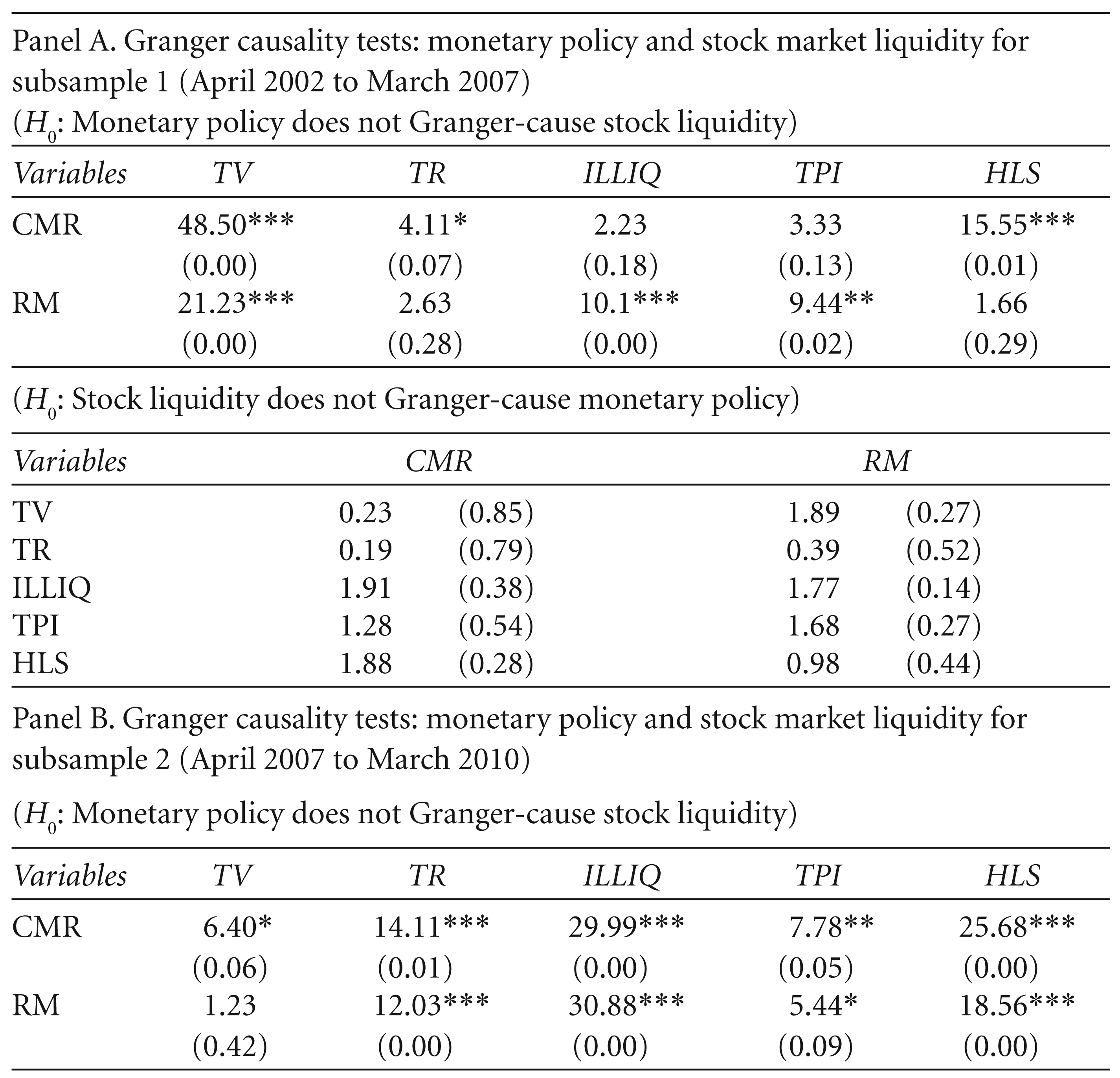
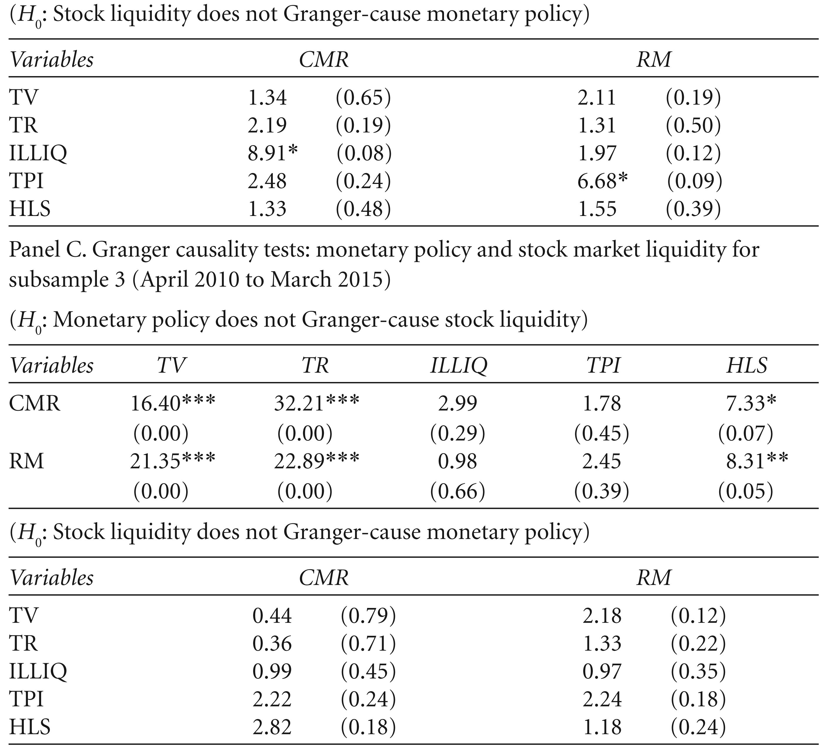
To check the consistency of our findings across normal market condition as well as during market turbulence, we further divide the sample period into three subsamples and carry out an analysis. The division of the data period is based on the occurrence of the recent global financial crisis. The first subsample period spans from April 2002 to March 2007 (the pre-crisis period); the second and third subsamples vary from April 2007 to March 2010 (during the crisis) and April 2010 to March 2015 (the post-crisis period), respectively.

The estimated results of the VAR–Granger causality tests between monetary policy and stock liquidity are reported in Table 6. In line with our earlier findings, we observe a significant flow of causality from monetary policy to stock liquidity across all periods. However, the effect is found to be more prominent during the crisis period. This could be due to the fact that the sudden drying-up of liquidity from the stock market during a financial crisis compels the monetary authority to take policy decisions to infuse liquidity into the financial system. For instance, an expansionary monetary policy (i.e., a decrease in the interest rate or increase in the money supply) reduces investors’ cost of borrowing and motivates them to trade actively in the market. The increased trading activities diminish the bid–ask spread and boost liquidity. We have observed that one of the illiquidity proxies Granger-causes monetary policy and it varies across the measures of monetary policy proxies. This could be due to the fact that during the crisis period, due to certain exogenous factors, the stocks of some companies become illiquid, which may affect the aggregate stock market performance adversely. Therefore, this compels policymakers to change policy rates like the repo rate to maintain the minimum level of liquidity, which ultimately affects other market-determined variables like the CMR, bank lending and also the aggregate money supply.

Table 6
Panel VAR–Granger Causality Tests for Monetary Policy and Stock Liquidity Across Subsamples

Panel A. Granger causality tests: monetary policy and stock market liquidity for subsample 1 (April 2002 to March 2007)
(H₀: Monetary policy does not Granger-cause stock liquidity)

Variables TV TR ILLIQ TPI HLS

CMR 48.50***
(0.00) 4.11*
(0.07) 2.23
(0.18) 3.33
(0.13) 15.55*
(0.01)

RM 21.23*
(0.00) 2.63
(0.28) 10.1*
(0.00) 9.44
(0.02) 1.66
(0.29)

(H₀: Stock liquidity does not Granger-cause monetary policy)

Variables CMR RM

TV 0.23 (0.85) 1.89 (0.27)

TR 0.19 (0.79) 0.39 (0.52)

ILLIQ 1.91 (0.38) 1.77 (0.14)

TPI 1.28 (0.54) 1.68 (0.27)

HLS 1.88 (0.28) 0.98 (0.44)

Panel B. Granger causality tests: monetary policy and stock market liquidity for subsample 2 (April 2007 to March 2010)
(H₀: Monetary policy does not Granger-cause stock liquidity)

Variables TV TR ILLIQ TPI HLS

CMR 6.40*
(0.06) 14.11*
(0.01) 29.99*
(0.00) 7.78
(0.05) 25.68*
(0.00)

RM 1.23
(0.42) 12.03*
(0.00) 30.88*
(0.00) 5.44*
(0.09) 18.56***
(0.00)

(H₀: Stock liquidity does not Granger-cause monetary policy)

Variables CMR RM

TV 1.34 (0.65) 2.11 (0.19)

TR 2.19 (0.19) 1.31 (0.50)

ILLIQ 8.91* (0.08) 1.97 (0.12)

TPI 2.48 (0.24) 6.68* (0.09)

HLS 1.33 (0.48) 1.55 (0.39)

Panel C. Granger causality tests: monetary policy and stock market liquidity for subsample 3 (April 2010 to March 2015)
(H₀: Monetary policy does not Granger-cause stock liquidity)

Variables TV TR ILLIQ TPI HLS

CMR 16.40*
(0.00) 32.21*
(0.00) 2.99
(0.29) 1.78
(0.45) 7.33*
(0.07)

RM 21.35*
(0.00) 22.89*
(0.00) 0.98
(0.66) 2.45
(0.39) 8.31**
(0.05)

(H₀: Stock liquidity does not Granger-cause monetary policy)

Variables CMR RM

TV 0.44 (0.79) 2.18 (0.12)

TR 0.36 (0.71) 1.33 (0.22)

ILLIQ 0.99 (0.45) 0.97 (0.35)

TPI 2.22 (0.24) 2.24 (0.18)

HLS 2.82 (0.18) 1.18 (0.24)

Panel A. Granger causality tests: monetary policy and stock market liquidity for subsample 1 (April 2002 to March 2007) (H₀: Monetary policy does not Granger-cause stock liquidity)
CMR	48.50*** (0.00)	4.11* (0.07)	2.23 (0.18)	3.33 (0.13)	15.55*** (0.01)
RM	21.23*** (0.00)	2.63 (0.28)	10.1*** (0.00)	9.44** (0.02)	1.66 (0.29)
(H₀: Stock liquidity does not Granger-cause monetary policy)

Variables	CMR	RM
TV	0.23 (0.85)	1.89 (0.27)
TR	0.19 (0.79)	0.39 (0.52)
ILLIQ	1.91 (0.38)	1.77 (0.14)
TPI	1.28 (0.54)	1.68 (0.27)
HLS	1.88 (0.28)	0.98 (0.44)
Panel B. Granger causality tests: monetary policy and stock market liquidity for subsample 2 (April 2007 to March 2010) (H₀: Monetary policy does not Granger-cause stock liquidity)

Variables	TV	TR	ILLIQ	TPI	HLS
CMR	6.40* (0.06)	14.11*** (0.01)	29.99*** (0.00)	7.78** (0.05)	25.68*** (0.00)
RM	1.23 (0.42)	12.03*** (0.00)	30.88*** (0.00)	5.44* (0.09)	18.56*** (0.00)
(H₀: Stock liquidity does not Granger-cause monetary policy)

Variables	CMR	RM
TV	1.34 (0.65)	2.11 (0.19)
TR	2.19 (0.19)	1.31 (0.50)
ILLIQ	8.91* (0.08)	1.97 (0.12)
TPI	2.48 (0.24)	6.68* (0.09)
HLS	1.33 (0.48)	1.55 (0.39)
Panel C. Granger causality tests: monetary policy and stock market liquidity for subsample 3 (April 2010 to March 2015) (H₀: Monetary policy does not Granger-cause stock liquidity)

Variables	TV	TR	ILLIQ	TPI	HLS
CMR	16.40*** (0.00)	32.21*** (0.00)	2.99 (0.29)	1.78 (0.45)	7.33* (0.07)
RM	21.35*** (0.00)	22.89*** (0.00)	0.98 (0.66)	2.45 (0.39)	8.31** (0.05)
(H₀: Stock liquidity does not Granger-cause monetary policy)

Variables	CMR	RM
TV	0.44 (0.79)	2.18 (0.12)
TR	0.36 (0.71)	1.33 (0.22)
ILLIQ	0.99 (0.45)	0.97 (0.35)
TPI	2.22 (0.24)	2.24 (0.18)
HLS	2.82 (0.18)	1.18 (0.24)

Source: Authors’ own computation.

Notes: This table presents the χ² statistics of pairwise panel Granger causality tests between monetary policy and stock liquidity across three subsample periods, that is, subsample 1 (April 2002 to March 2007), subsample 2 (April 2007 to March 2010) and subsample 3 (April 2010 to March 2015). The corresponding p-values are given in parentheses. ***, ** and * show significance at the 1%, 5% and 10% levels, respectively.

7. Conclusions

This study examines the relationship between monetary policy and stock liquidity over the period 2002 through 2015 in a pure order-driven emerging stock market like India. We use five different liquidity measures to capture several aspects of liquidity such as trading activity, price impact and transaction cost. Monetary policy is approximated by the CMR and 12-month growth rate of reserve money. To ascertain the relationship between monetary policy and stock liquidity, we conducted a panel VAR–Granger causality test, IRF and variance decomposition analysis.

The Granger causality test indicates that monetary policy significantly Granger-causes stock liquidity; however, we do not find much evidence for the reverse. It is evident from the impulse response analysis that an expansionary monetary policy, which is characterised by a lower interest rate or higher money supply, enhances stock liquidity. The variance decomposition analysis reveals that the monetary policy explains a larger portion of variation in stock liquidity. Overall, we document a strong predictability of monetary policy on stock liquidity. This may be used as a determinant of observed commonality in the liquidity of individual stocks and to understand the cross-sectional variations of liquidity in the stock market. The impact of monetary policy on stock liquidity is more and there is a weak bidirectional causality between monetary policy and stock illiquidity in the crisis period.

The findings of the present study have certain theoretical as well as practical implications. Market participants in an equity market can improve the forecasting of liquidity in their investment portfolios by employing monetary policy along with individual asset characteristics. Regulators and policymakers may consider the cross-sectional relationship between stock liquidity and monetary policy as an important source of information for policy formulation and implementation. The focus of our study is limited to exploring the role of monetary policy on stock liquidity. But we have not touched upon the channels through which monetary policy transmits its effects to stock liquidity. Our work may be considered a baseline study to further explore in these areas.

Declaration of Conflicting Interests

The authors declared no potential conflicts of interest with respect to the research, authorship and/or publication of this article.

Funding

The authors received no financial support for the research, authorship and/or publication of this article.

References

Abrigo

M. R. M.

& Love

(2016). Estimation of panel vector autoregression in Stata. Stata Journal, 16(3), 778–804.

Acharya

& Pedersen

L. H.

(2005). Asset pricing with liquidity risk. Journal of Financial Economics, 77(2), 375–410.

Acharya

& Schaefer

(2006). Liquidity risk and correlation risk: Implications for risk management. Retrieved from http://pages.stern.nyu.edu/~sternfin/vacharya/public_html/acharya_schaefer2.pdf

Aleem

(2010). Transmission mechanism of monetary policy in India. Journal of Asian Economics, 21(2), 186–197.

Amihud

(2002). Illiquidity and stock returns: Cross-section and time-series effects. Journal of Financial Markets, 5(1), 31–56.

Amihud

& Mendelson

(1986). Asset pricing and the bid-ask spread. Journal of Financial Economics, 17(2), 223–249.

Amihud

& Mendelson

(1989). The effect of beta bid-ask spread, residual risk, and size on stock returns. Journal of Finance, 44(2), 479–486.

Amihud

Mendelson

Pedersen

L. H.

(2005). Liquidity and asset prices. Foundation and Trends in Finance, 1(4), 269–364.

Atje

& Jovanovic

(1993). Stock markets and development. European Economic Review, 37 (2–3), 632–640.

10.

Bekaert

& Harvey

C. R.

(2003). Emerging markets finance. Journal of Empirical Finance, 10(1–2), 3–55.

11.

Borio

(2004). Market distress and vanishing liquidity: Anatomy and policy, options (BIS Working Papers No. 158). Bank of International Settlements. Retrieved from http://www.bis.org/publ/work158.html

12.

Brennan

M. J.

Chordia

& Subrahmanyam

(1998). Alternative factor specifications, security characteristics, and the cross-section of expected stock returns. Journal of Financial Economics, 49(3), 345–373.

13.

Brunnermeier

M. K.

& Pedersen

L. H.

(2009). Market liquidity and funding liquidity. Review of Financial Studies, 22(6), 223–249.

14.

Chordia

Roll

& Subrahmanyam

(2000). Commonality in liquidity. Journal of Financial Economics, 56(1), 3–28.

15.

Chordia

Roll

& Subrahmanyam

(2001). Market liquidity and trading activity. Journal of Finance, 56(2), 501–530.

16.

Chordia

Sarkar

& Subrahmanyam

(2005). An empirical analysis of stock and bond market liquidity. Review of Financial Studies, 18(1), 85–130.

17.

Chu

(2015). Modelling impact of monetary policy on stock market liquidity: A dynamic copula approach. Applied Economics Letters, 22(10), 820–824.

18.

Copeland

T. E.

& Galai

(1983). Information effects on the bid-ask spread. Journal of Finance, 38(5), 1457–1469.

19.

Corwin

S. A.

& Schultz

(2012). A simple way to estimate bid-ask spread from daily high-low prices. Journal of Finance, 67(2), 719–759.

20.

Das

& Hanouna

(2009). Hedging credit: Equity liquidity matters. Journal of Financial Intermediation, 18(1), 112–123.

21.

Datar

V. T.

Naik

Y. N.

& Radcliffe

(1998). Liquidity and stock returns: An alternative test. Journal of Financial Markets, 1(2), 203–219.

22.

Dhal

(2000). Short-term interest rates and real economic activity. Reserve Bank of India Occasional Paper, 21(1), 61–78.

23.

Dickey

& Fuller

(1981). Likelihood ratio statistics for autoregressive time series with a unit root. Econometrica, 49(4), 1057–1072.

24.

Eisfeldt

A. L.

(2004). Endogenous liquidity in asset markets. Journal of Finance, 59(1), 1–30.

25.

Fernandez-Amador

Gächter

Larch

& Perter

(2013). Does monetary policy determine stock market liquidity? New evidence from the euro zone. Journal of Empirical Finance, 21(1), 54–68.

26.

Florakis

Gregoriou

& Kostakis

(2011). Trading frequency and asset pricing on the London Stock Exchange: Evidence from a new price impact ratio. Journal of Banking and Finance, 35(12), 3335–3350.

27.

Fujimoto

(2003). Macroeconomic sources of systematic liquidity. Retrieved from http://www.ibrarian.net/navon/paper/Macroeconomic_Sources_of_Systematic_Liquidity.pdf?paperid=226950

28.

Garcia

(1989). The lender of last resort in the wake of the crash. American Economic Review, 79(2), 151–155.

29.

Goyenko

R. Y.

& Ukhov

A. D.

(2009). Stock and bond market liquidity: A long-run empirical analysis. Journal of Financial and Quantitative Analysis, 44(1), 189–212.

30.

Goyenko

R. Y.

Holden

C. W.

& Trzcinka

C. A.

(2009). Do liquidity measures measure liquidity? Journal of Financial Economics, 92(2), 153–181.

31.

Granger

C. W. J.

(1969). Investigating causal relations by econometric models and cross-spectral methods. Econometrica, 37(3), 424–438.

32.

Hameed

Kang

& Viswanathan

(2010). Stock market declines and liquidity. Journal of Finance, 65(1), 257–293.

33.

Hasbrouck

(2007). Empirical market microstructure: The institutions, economics, and econometrics of security trading. New York: Oxford University Press.

34.

Haugen

R. A.

& Baker

N. L.

(1996). Commonality in the determinants of expected stock returns. Journal of Financial Economics, 41(3), 401–439.

35.

Holtz-Eakin

Newey

& Rosen

H. S.

(1988). Estimating vector auto regressions with panel data. Econometrica, 56(6), 1371–1395.

36.

Huberman

& Halka

(2001). Systematic liquidity. Journal of Financial Research, 24(2), 161–178.

37.

K. S.

Pesaran

M. H.

& Shin

(2003). Testing for unit roots in heterogeneous panels. Journal of Econometrics, 115(1), 53–74.

38.

Jun

S.-G.

Marathe

& Shawky

H. A.

(2003). Liquidity and stock returns in emerging equity markets. Emerging Markets Review, 4(1), 1–24.

39.

Korajczyk

R. A.

& Sadka

(2008). Pricing the commonality across alternative measures of liquidity. Journal of Financial Economics, 87(1), 45–72.

40.

Kyle

A. S.

(1985). Continuous auctions and insider trading. Econometrica, 53(6), 1315–1335.

41.

Lesmond

D. A.

(2005). Liquidity of emerging markets. Journal of Financial Economics, 77(2), 411–452.

42.

Levin

Lin

C.-F.

& Chu

C. S. J.

(2002). Unit root tests in panel data: Asymptotic and finite-sample properties. Journal of Econometrics, 108(1), 1–24.

43.

Levine

& Zervos

(1998). Capital control liberalisation and stock market development. World Development 26(7), 1169–1183.

44.

& Mackinlay

(1990). Data-snooping biases in tests of financial asset pricing models. Review of Financial Studies, 3(3), 431–467.

45.

Love

& Zicchino

(2006). Financial development and dynamic investment behaviour: Evidence from panel VAR. Quarterly Review of Economics Finance, 46(2), 190–210.

46.

Mishra

& Mishra

(2012). Evaluating inflation targeting as a monetary policy objective for India. Economic Modelling, 29(4), 1053–1063.

47.

Næs

Skjeltorp

J. A.

& Ødegaard

B. A.

(2011). Stock market liquidity and the business cycle. Journal of Finance, 66(1), 139–176.

48.

National Stock Exchange of India (2015). Indian securities market, a review. Mumbai, India: National Stock Exchange of India.

49.

O’Hara

(1998). Market microstructure theory. Cambridge, MA: Blackwell.

50.

Pastor

& Stambaugh

R. F.

(2003). Liquidity risk and expected stock returns. Journal of Political Economy, 111(3), 642–685.

51.

Prabu

E. A.

Bhattacharyya

& Ray

(2016). Is the stock market impervious to monetary policy announcements? Evidence from emerging India. International Review of Economics and Finance, 46, 166–179.

52.

Ray

& Prabu

E. A.

(2013). Financial development and monetary policy transmission across financial markets: What do daily data tell for India? (RBI Working Paper No. DEPR/04/2013). Reserve Bank of India. Retrieved from https://www.rbi.org.in/scripts/PublicationsView.aspx?id=14985

53.

Sarr

& Lybek

(2002). Measuring liquidity in financial markets (IMF Working Paper No. WPS/02/232). International Monetary Fund. Retrieved from http://www.imf.org/en/Publications/WP/Issues/2016/12/30/Measuring-Liquidity-in-Financial-Markets-16211

54.

Soderberg

(2008). Do macroeconomic variables forecast changes in liquidity? An out-of-sample study on the order-driven stock markets in Scandinavia (CAFO Working Paper Series-2009/10). Centre for Labour Market Policy Research. Retrieved from http://www.ibrarian.net/navon/paper/Centre_for_Labour_Market_Policy_Research.pdf?paperid=14870079

55.

Stoll

H. R.

(1978). The pricing of security dealer services: An empirical study of Nasdaq stocks. Journal of Finance, 33(4), 1153–1172.

56.

The World Bank (2016). World development indicators. Washington, DC: The World Bank.

57.

Trichet

J. C.

(2010). The great financial crisis: Lessons for financial stability and monetary policy. In Constâncio

(Ed.), The great financial crisis (pp. 7–11). Frankfurt am Main, Germany: Colloquium Conducted in Honour of Lucas Papademos at the Meeting of European Central Bank.

58.

Wang

(2013). Liquidity commonality among Asian equity markets. Pacific-Basin Finance Journal, 21(1), 1209–1231.

59.

Wooldridge

J. M.

(2002). Introductory econometrics: A modern approach. Mason, OH: Cengage Learning.