



Abstract
According to the neoclassical economists, discrimination exists in the labour market if employers treat two equally qualified and skilled persons differently based on gender, race, age, disability, religion, caste, etc. In this article, we attempt to look at discrimination in the Indian labour market by applying the multinomial probit model of regression to the National Sample Survey Office data set. By taking years of schooling (as an indicator of skill and ability) as an independent variable in the model, we find that identically educated persons from different caste and gender groups are not equally likely to achieve similar occupational status, indicating the existence of discrimination in the Indian labour market.
Introduction
Occupational status can influence the health and self-esteem of individuals and improve earnings, consumption and the general status of households (Harper & Haq, 1997). Thus, occupational attainment can influence economic development by achieving egalitarian distribution of income and wealth (Banerjee & Newman, 1993). According to a priori reasoning and findings of a substantial number of studies, occupational attainment and earning of an individual depends on his/her educational achievement, area of study and work experience (Becker, 1957; Mincer, 1958; Shabbir, 1993; Shields & Stephen, 2002). However, in practice employers may treat two equally qualified and skilled persons distinctly on account of their gender, race, caste, etc. This implies better educational achievement does not always enable a person to achieve a better occupation. In any society, the existing occupational disparity can be treated as occupational discrimination if this disparity occurs due to the prejudice and differential treatment of the employers (Arrow, 1972a, 1972b; Becker, 1957; Phelps, 1972). In the absence of discrimination in the labour market, the between-group occupational disparity can be reduced through the implementation of effective compensation policies. But discrimination-led occupational disparity cannot be reduced by straightforward policy implementation, and this occupational disparity leads to a decline in the well-being of the members of the groups who are discriminated against.
Gender group disparity is also common across societies (Bayard et al., 2003; Blau et al., 2013; Teo, 2003; Zveglich & Rodgers, 2004). According to the findings of these studies, in different societies males are usually concentrated at the top of the occupational hierarchy compared to females, that is, males are employed in high-paying occupations compared to females, even though both genders are equally rational in the context of occupational choice. This may be the consequence of a disparity in educational achievement and/or it may be attributed to discrimination in the labour market, which prevents females from entering high-paying occupations even with better education (Baldwin et al., 2001; Higginbotham & Weber, 1999). In the context of India, Kingdon and Unni (2001) find that women face wage discrimination in the Indian urban labour market even if their returns to education are greater than men, as the contribution of education to discrimination against women is negligible.
Caste is the most significant social grouping, segregating Indian society broadly into four social groups: Higher Castes (HCs), Other Backward Castes (OBCs), Scheduled Castes (SCs) and Scheduled Tribes (STs). This classification was initially done on the basis of occupation, and members of the SCs were systematically concentrated at the bottom of the occupational hierarchy, which resulted in poor earnings of the members of this group. The HC members were concentrated at the top of social hierarchy and owned or controlled the land and possessed the power. The lower castes provided services for the HCs, and in return, they received payment for maintaining their livelihoods. Consequently, successive generations of the members of lower caste groups inherently had lower opportunities which hindered them from participating in education or continuing education after a certain level; group disparity persists in education, employment and income. The persistence of group disparities in different dimensions can be observed from the findings of a considerable number of studies (Desai & Kulkarni, 2008; Deshpande, 2001; Gang et al., 2017; Government of India, 2006; Kijima, 2006).
It is worth mentioning that current disparities in occupation among the social groups cannot be entirely attributed to unequal opportunities and poor educational achievements of members of the deprived social groups. Findings of different studies reveal that an employer’s preference is one of the reasons behind occupational disparity among social groups. Madheswaran and Attewell (2007) find that members of disadvantaged social groups are discriminated against both in public and private sector jobs, with greater discrimination in the latter, and all jobs are not equally accessible to members of all social groups. Another study conducted by Agrawal (2014) notices wage discrimination against women and disadvantaged social groups in the Indian labour market.
Almost all the existing studies on labour market discrimination in different countries as well as in India assess discrimination in terms of wage earnings between two major groups, such as between males and females, whites and blacks, SCs and non-SCs and so on. Most of these studies apply the method of decomposition of wage disparity suggested by Oaxaca (1973) and Blinder (1973). This method allows computing the scalar value of discrimination in wage earnings when there is no educational disparity as well no difference in other endowments. Therefore, this method does not allow us to explain whether identically educated people are equally able to get better jobs and wages, that is, the contribution of education to labour market discrimination. Jobs at the top of the occupational hierarchy do provide better not only wage earnings but also occupational conditions. Therefore, better jobs mean better wages, but the converse is not strictly true, and a separate analysis of job discrimination is necessary, for which the Oaxaca–Blinder method cannot be applied in a straightforward way, as occupation is a nominal categorical variable. Furthermore, through this method of decomposition, wage discrimination between two major groups can be assessed. Therefore, it fails to display the actual discrimination in the labour market when more than two groups are identified
In the light of the existing studies, we attempt to look at existing job discrimination against the disadvantaged social groups in India, based on the neoclassical view of labour market discrimination, that is, we examine whether equally qualified and skilled persons across different social groups have identical access to jobs suited to their specific educational levels. For this, we classify jobs into three categories according to the status of different jobs in the occupational hierarchy, ‘white-collar jobs’, ‘pink-collar jobs’ and ‘blue-collar jobs’, and run the multinomial probit (MNP) model of regression separately for the rural and urban samples, taking education as the main independent variable. In addition, we segregate the sample by taking caste and gender together and run the MNP regression separately for this classification. This will enable us to articulate the actual condition of occupational discrimination against the deprived social groups and females in the Indian labour market more critically. To the best of our knowledge, the method employed in this study is different from the existing studies on labour market discrimination.
The rest of this article is structured as follows. Section 2 describes the data source, the methodology employed and the variables included in the regression analysis employed in the study. Section 3 explains the results, and Section 4 discusses the findings and concludes.
Data and Methods
Data Source
This study draws on the data set from the Household Employment and Unemployment Survey conducted by the National Sample Survey Office (NSSO) of India in 2011–2012. We have included household characteristics, such as social group (i.e., caste) and religion, and individual characteristics such as gender, level of education, working status, relationship to household head and occupational group if working, and community characteristics such as region and sector of residence in our analysis.
The NSSO survey provides information on around 500,000 individuals from various religious groups. We restrict our sample to Hindus. 1 The data sets provided do not contain the information on parental education and occupation or on the family background of the respondents but this can be obtained from information on the relationship of the individual with the head of their family. Three sets of fathers and offspring can be developed from this information: (a) household heads and their children (if the household head is male), (b) household heads and their fathers (if the parent is male) and (c) children and grandchildren of the household heads. Complete information on the educational qualification and occupational status of fathers can be obtained from the serial numbers of the households and persons, which are available in the data sets. One limitation of this method of collecting information on fathers is that it does not allow us to get information on father’s education and occupation of individuals living in a one-member household, two-member household (husband and wife) and nuclear household (husband, wife and young children), so we drop these households from the analysis. This reduces the sample size to around 190,000 individuals. This sample is further reduced, as we include only those between 25 and 65 years who have completed their education to 60,000 individuals and even further to 31,000 as we include only full-time working individuals based upon their responses on their principal activity status. 2
Econometric Model
To examine the existence of discrimination in the Indian labour market, we assess the influence of educational attainment on occupational status. For this, we employ a discrete choice model, where the dependent variable has more than two categories and an individual chooses one category (one type or category of occupation).
This discrete choice model can be explained by the random utility theory. If there are n (i = 1, 2,…, n) individuals and m (j = 1, 2,…, m) alternative categories of the outcome variable, an individual decision-maker chooses the alternative out of m from which he/she obtains maximum utility. In the random utility theory, utility (or indirect utility) depends on two components, one known to the decision-maker and the other which is random and unknown to the decision-maker. The first component is observable and the second is unobservable to the decision-maker. So, the utility function of the decision-maker can be written as:

Where Ui is the utility from the ith alternative of the response variable; Vi is the observed or systematic component of utility of ith alternative of the response variable and εi is the stochastic component of utility. If there are n alternatives of the response variable, then the decision-maker faces a choice among these alternatives. For non-zero value of

To estimate the influence of the factors on the choice of a particular alternative category of outcomes, researchers typically employ the conditional logit model for ordinal categories of the dependent variable or its special variant multinomial logit (MNL) model of regression for nominal categories of the dependent variable. This MNL model is easy to estimate, and interpretation of the coefficients is straightforward; the only complication is the analysis of the results due to the existence of a large number of parameters. However, researchers and scholars have shown that one complicated and impractical assumption known as the independence of irrelevant alternatives (IIA) is implicit in the MNL (Alvarez & Nalgler, 1995; Lacy & Burden, 1999; Mokhtarian & Bagley, 2000). 3 The MNP model is free from the IIA assumption and can be applied for the nominal categorical dependent variable where there are more than two similar alternatives of the dependent variable.
Researchers frequently use the MNL model of regression as they have not paid any attention to the dependence of the MNL model on the independence of the IIA assumption. 4 Since the MNL model is associated with the IIA assumption, we use the MNP model of regression in this study to look at the influence of education and other variables on occupational choice in India. This enables us to explain the existing discrimination in the Indian labour market.
If there are K alternatives of the outcome/dependent variable in the MNP model of regression, that is, K categories of occupation for the analysis of occupational choice, then the probability that an individual (say, i) characterized by the vector of n number of independent variables, such as

Initially, to look at the impacts of different predictor variables on occupational status and the existence of discrimination in the Indian labour market, we apply the MNP model of regression separately for the rural and urban samples. 5 However, for more insight into the actual reason for discrimination in the Indian labour market, we run five additional multinomial regressions by taking more than one predictor variable together. Therefore, we run a total of seven MNP regressions in this study.
By reshuffling the order of occupational categories given in Ministry of Labour and Employment, 2004, and following the method of occupational classifications in Azam (2013), we develop three hierarchical classifications based upon skills and status of occupations.
6
(We drop cultivators and farmers other than cultivators from our analysis to avoid ambiguity in the ranking of occupations.) The three categories are, ‘blue-collar jobs’, ‘pink-collar jobs’ and ‘white-collar jobs’. The first category comprises unskilled jobs, the second consists of skilled and semi-skilled jobs and the third category included high-skilled and sophisticated jobs. These three categories of occupations can be arranged in an ascending order according to skills and prestige in the following way:
Blue-collar jobs: Hotel and restaurant workers, housekeepers, building caretakers, service workers, other farm workers, forestry workers, etc. Pink-collar jobs: Village officials, clerical, transport and communication supervisors, stenographers, typist, bookkeepers, telephone and telegraph operators, manufacturers, agents, etc. White-collar jobs: Physical scientists, engineering technicians, physicians and surgeons, economists and related workers, social scientists, teachers, professional workers, etc.
Variables Included in the Multinomial Probit Regression
As mentioned, to examine for the existence of discrimination in the labour market we include educational status (measured in terms of years of formal schooling) as an explanatory variable in the MNP model of regression. However, in the NSSO data sets, educational achievement is measured by completed levels of education. Therefore, educational achievement is categorical in nature. If we take education as a categorical variable in the MNP regression, then we can explain the likelihood of employment of the persons or groups who have completed a specific level of education in a particular category of job rather than other categories of jobs, compared to persons or groups having the reference level of education. By taking education as a categorical variable it is not possible to evaluate the overall influence of education on occupational attainment. Thus, to examine the overall impact of education on occupational choice we have to consider education as a cardinal variable and therefore convert levels of education into years of education. 7
To analyse the existing occupational disparity among caste groups, we include social group as an explanatory variable. This variable has four categories, with ‘HCs’ as the reference category in the regression equation. To examine the existence of discrimination, that is, the differential impact of education on occupational status, the interaction terms between years of education and the categories of social groups are taken as another categorical predictor variable. This interaction dummy has four categories: HCs and education, OBCs and education, SCs and education, and STs and education (with the dummy HCs and education included in the regression equation as the reference category).
To investigate gender-based occupational disparity, gender is included as a categorical predictor variable, with males as the reference category. Negative discrimination against female workers in the Indian labour market is analysed through the interaction terms between gender and years of education in the regression equation. In addition, to assess the influence of family background on the occupational attainment of an individual, the regression equation includes as a categorical independent variable father’s education, of which there are three categories: ‘low educated’, if the father is illiterate or has no formal schooling or has only completed schooling up to the middle level; ‘moderately educated’, if the father has completed the secondary or higher secondary level of education and ‘high educated’, if they are graduates, postgraduates or a diploma-holder. We take ‘low-educated’ fathers as the reference category in the regression.
To identify inequality in existing discrimination in the rural and urban areas, we run two separate regression equations, for the rural and urban areas. In addition, as males and females are not alike across all social groups, we run a separate probit regression by taking the interaction term between sector and gender.
Results
Descriptive Statistics
Only 4.4 per cent and 19.54 per cent of the total sample are in the first category of occupation in the rural and urban areas, respectively, which needs the highest level of skill (Table 1). The population shares of the second and third occupational categories are 5.23 per cent and 90.37 per cent in the rural areas, and 21.06 per cent and 58.50 per cent in the urban areas, respectively.
Sample Characteristics, NSSO, 2011–2012 (Percentages)
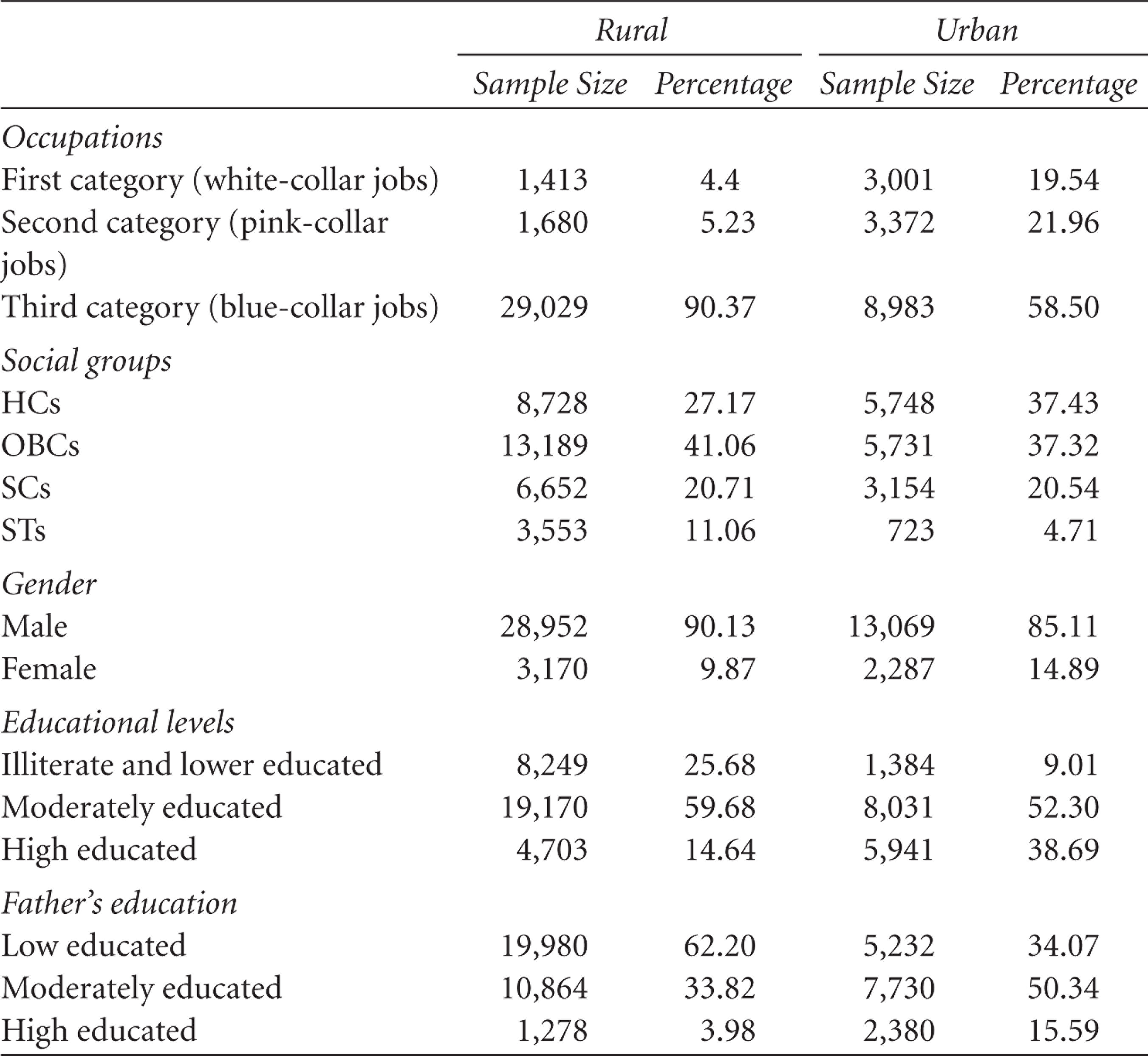
Sample Characteristics, NSSO, 2011–2012 (Percentages)
From the reported numerical figures, it is clear that a major share of the rural and urban population falls in the second category of education (59.8% and 52.3%, respectively). A rural-urban gap is indicated by the population shares in first and third categories of education, since in the rural areas more people are low educated or uneducated, and in the urban areas more individuals are high educated. The analysis of father’s education shows that in the rural areas most people are the sons of low-educated or uneducated fathers, whereas the in urban areas a significant percentage are sons of moderately educated fathers.
Table 2 presents the results of the bivariate analysis, where we distribute the population by social groups, gender and family background (measured by father’s education) across three occupational categories separately for the rural and urban samples. Social groups, gender and father’s education are the regressors in the MNP model of regression, to assess occupational discrimination in the Indian labour market. We also tested the association between caste and occupational categories, gender and occupational categories, and father’s education and occupational categories using the Pearson’s chi-square statistic (not reported in the tables) and have found a statistically significant difference in occupational choices between groups defined by caste, gender and father’s education.
It is also observed that a larger proportion of population across social groups is concentrated at the bottom of the occupational ladder both in the rural and urban areas, for all types of classification: caste, gender, educational level and father’s education (Table 2). Even if the concentration of different social groups across occupational categories is identical, the members of the HCs are in a relatively better position in the occupational hierarchy both in the rural and urban areas, as the percentage of HCs employed in ‘white-collar jobs’ is greater than the other social groups, and its population proportion in ‘blue-collar jobs’ is smaller than the other social groups. In terms of the concentration of population in different categories of occupations, the OBCs occupy the lowest rank in the rural areas, and the same position is occupied by SCs in the urban areas.
Distribution of Population by Occupational Category

The distribution of males and females across occupational categories reveals that gender disparity is greater in urban areas than in rural areas. The distribution of each educational group across occupational categories shows that only one in 1,000 illiterate and uneducated persons are employed in the highest category of occupation, and 214 out of 1,000 high-educated persons can get employment in the highest category of occupation in the rural areas; these figures are 20 out of 1,000 and 239 out of 1,000 in the urban areas, respectively. Therefore, education has a strong bearing on occupational achievement, as the increase in educational achievement almost immediately improves the occupational status of individuals. Further, only 2.25 per cent of the sons of ‘uneducated and low-educated’ fathers are able to get a job in the highest category of occupation, but 16.3 per cent of the sons of ‘higher-educated’ fathers are able to occupy the topmost position in the occupational ladder in the rural areas; in the urban areas, these figures are 5 per cent and 19.2 per cent, respectively. Therefore, the distribution of populations defined by father’s education across occupational categories reveals that father’s education has a strong bearing on the occupational achievement of the offspring.
The results of the econometric estimation are reported in Tables 3, 4a and 4b. There are two sets of coefficients and z-values of each MNP model of regression for the rural and urban samples for three categories of categorical response variables. In the first case, the MNP model of regression estimates the likelihood of attaining a ‘white-collar job’ rather than a ‘blue-collar job’, and in the second case, the regression estimates the likelihood of attaining a ‘pink-collar job’ rather than a ‘blue-collar job’ (these cases are named as ‘white-collar jobs’ and ‘pink-collar jobs’ where the reference category is ‘blue-collar jobs’ for each case).
The coefficients of ‘years of schooling’ across all regressions are positive and significant, which indicates that an increase in educational achievement raises the probability of achieving a better outcome in the rural and urban labour markets. Controlling for other variables, a sharp disparity in occupational status across the social groups can be observed. The estimated coefficients of the dummies for SCs and STs reveal that they are less likely to be employed in ‘white-collar jobs’ than in ‘blue-collar jobs,’ compared to members of the HCs in both the rural and urban samples. Likewise, SCs and STs are less likely to be employed in ‘pink-collar jobs’ than in ‘blue-collar jobs’ compared to HCs in the rural areas, though this disparity between the disadvantaged social groups and HCs in the context of being employed in ‘pink-collar jobs’ than in ‘blue-collar jobs’ disappears in the urban areas. The signs and magnitudes of the estimated coefficients of the dummy for OBCs in all regressions reveal a disparity between OBCs and HCs only in the likelihood of getting employment in ‘white-collar jobs’ rather than in ‘blue-collar jobs’ but not in ‘blue-collar jobs’ rather in ‘blue-collar jobs’ in the rural sector.
The estimated coefficients of the interaction terms between social group dummies and ‘years of schooling’ reveal that in the urban areas an increase in human capital formation augments the probability of getting ‘white-collar jobs’ over ‘blue-collar jobs’ for those from the so-called socio-economically disadvantaged social groups the OBCs, SCs and STs, compared to the HCs. In the rural sample, this disparity persists only for OBCs, and in fact is reversed for SCs and STs, as the estimated values of the coefficients of SCs and education and STs and education reveal that educated SCs and STs in rural areas are less likely to be employed in ‘white-collar jobs’ than in ‘blue-collar jobs’ compared to the educated HCs. This disparity in the contribution of education to occupational achievement among social groups across rural and urban areas may be the consequence of a disparity in job accessibility.
Results of the Multinomial Probit Model for Occupational Choice

Results of the Multinomial Probit Model for Occupational Choice
Results of the Multinomial Probit Model for Occupational Choice
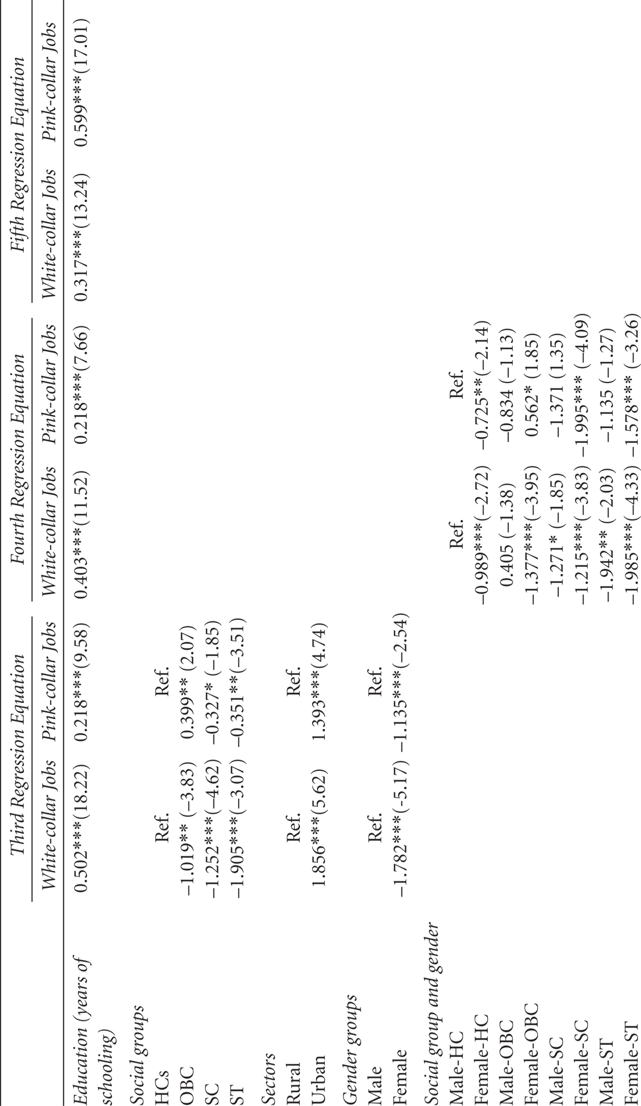
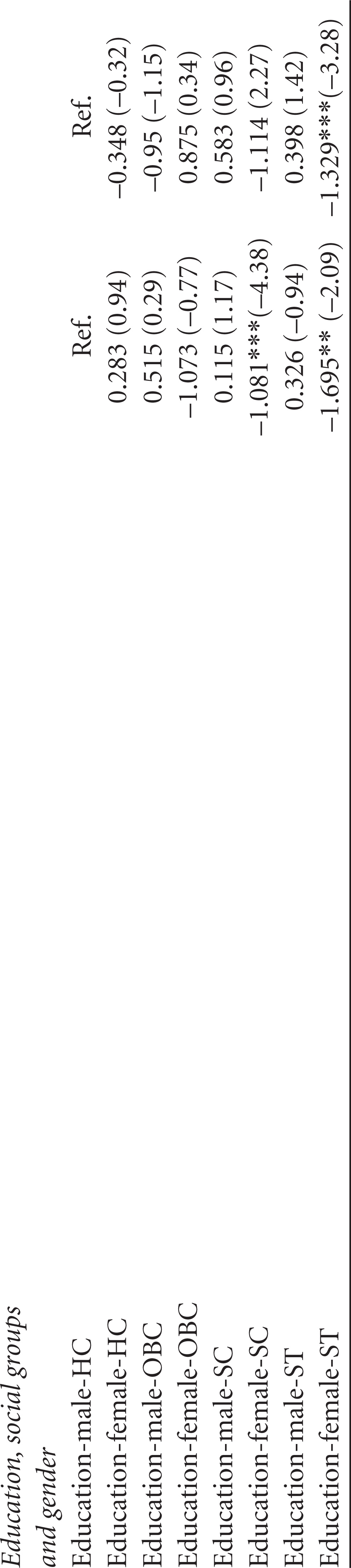
Results of the Multinomial Probit Model for Occupational Choice
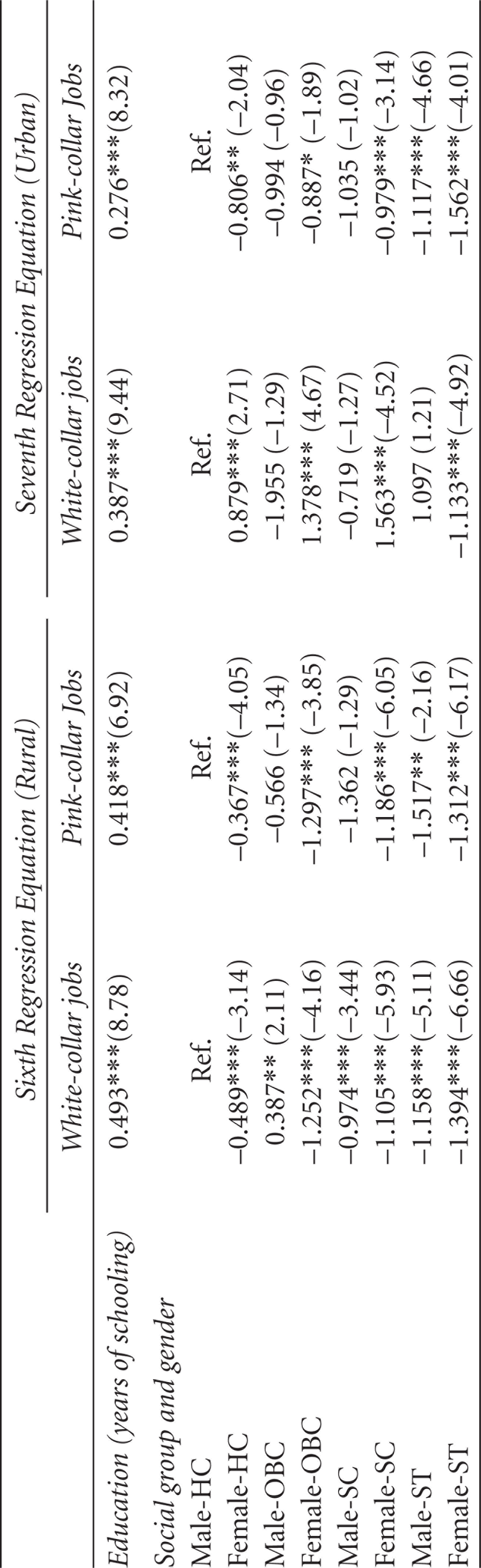
Education also plays different roles for different social groups in getting employment in ‘pink-collar jobs’, since educated SCs and STs are less likely to be employed in these jobs rather than in ‘blue-collar jobs’ compared to HCs in rural areas. However, in urban areas, the disparity in the contribution of education to employment in ‘pink-collar jobs’ rather than in ‘blue-collar jobs’ exists only between STs and HCs, that is, a rise in education raises the likelihood of getting ‘pink-collar jobs’ rather than ‘blue-collar jobs’ for STs compared to HCs, but there is no disparity between OBCs and HCs, and SCs and HCs in this regard. Based upon these results, it can be stated that education has a more beneficial effect on disadvantaged social groups in the urban areas compared to advantaged social group HCs, though it is not uniformly true in the rural areas.
The estimated values of the female dummy in the regression equation for the rural sample reveal that females are significantly less likely to be employed in ‘white collar-jobs’ and in ‘pink-collar jobs’ than in ‘blue-collar jobs’ compared to males in the rural areas. This is reversed in the urban areas, since the estimated value of the female dummy reveals that in urban areas females are significantly more likely to be employed in ‘white collar-jobs’ rather than ‘blue-collar jobs’ compared to males. These results are not in complete conformity with the findings of some earlier studies on occupational choice (Bayard et al., 1999; Blau & Khan, 1996; Zveglich & Rodgers, 2004). This dominance of females over males in urban areas may be the consequence of reservation policies or the outcome of better household economic status in urban areas compared to rural areas. In fact, the better household economic status may be an important reason behind the better educational status of females in urban areas, which enables them to attain a better position in the occupational hierarchy. However, the estimated value of the female dummy in the regression equation for the urban sample reveals that females are less likely to be employed in ‘pink-collar jobs’ than in ‘blue-collar jobs’ compared to males in urban areas. Therefore, males dominate in getting employment in ‘pink-collar jobs’ in urban areas.
Another finding is that education significantly and consistently influences the likelihood of occupational attainment between males and females. Higher-educated females are less likely to get ‘white-collar jobs’ or ‘pink-collar jobs’ compared to males both in rural and urban areas. Further, the estimated coefficients of the interaction term between the female dummy and years of education are negative and significant, which indicates that the rise in the years of schooling reduces the likelihood of female employment at the top of the occupational hierarchy.
Lastly, in the rural areas, father’s education significantly and consistently influences the likelihood of getting ‘white-collar jobs’ but not the likelihood of getting ‘pink-collar jobs’. In urban areas, the finding is quite different, as here the influence of father’s education on the occupational attainment of sons is not consistent.
Finally, the classification of the population taking caste and gender together gives a clearer picture of occupational discrimination. We consider three separate regression equations for the national data, that is, by combining the rural and urban samples. In the third regression equation, we take education, caste, sector and gender as the predictor variables; in the fourth regression equation we consider education and the combination of caste and gender as the independent variables; and in the fifth regression equation, we include education and the combination of education, caste and gender as the independent variables in the analysis.
According to the estimation results of the third regression equation, a rise in educational achievement raises the probability of getting employment in ‘white-collar jobs’ rather than ‘blue-collar jobs’, and it also raises the likelihood of getting employment in ‘pink-collar jobs’ rather than in ‘blue-collar jobs’. Educated HCs are significantly more likely to be employed in ‘white-collar jobs’ than ‘blue-collar jobs’ compared to OBCs, SCs and STs. However, there is no significant difference between HCs and OBCs in the likelihood of getting employment in ‘pink-collar jobs’ rather than ‘blue-collar jobs’, though in this case also, SCs and STs are less likely to get these jobs than HCs. Females are significantly less likely than males to get ‘white-collar jobs’ rather than ‘blue-collar jobs’. Likewise in the first case (i.e., the part of regression of the ‘white-collar jobs’), females are significantly less likely to get ‘pink-collar jobs’ than ‘blue-collar jobs’. Lastly, the estimated coefficients of the third regression equation reveal that urban residents are more likely to be employed in ‘white-collar jobs’ than in ‘blue-collar jobs’ and in ‘pink-collar jobs’ rather than in ‘blue-collar jobs’ compared to rural residents.
The estimated values of the coefficients of education in both cases of the fourth regression equation are positive and significant, which corroborate the findings of the previous three regression equations. A significant fact emerges from the results of the fourth regression equation that there is no significant difference in the likelihood of getting employment in ‘white-collar jobs’ rather than ‘blue-collar jobs’ between HCs-males and OBCs-males, but there is explicit and significant gender disparity across HCs and OBCs. Females in each of these groups are less likely to be employed in ‘white-collar jobs’ rather than in ‘blue-collar jobs’ compared to males. This dominance of HCs-males and OBCs-males in getting employment in ‘white-collar jobs’ rather than in ‘blue-collar jobs’ over HCs-females and OBCs-females does not substantiate the findings of the second regression equation. This gender disparity disappears in the samples of SCs and STs.
To reconcile these two contradictory results, we run two additional MNP model of regressions separately for the rural and urban samples and include the interaction term between gender and caste as the predictor variable along with education (i.e., sixth and seventh regression equations). The results of the estimation of the sixth regression equation reveal that in the rural areas, OBCs-males are more likely to be employed in ‘white-collar jobs’ rather than in ‘blue-collar jobs’ compared to HCs-males. According to these results, there is inter-caste disparity in the likelihood of getting ‘white-collar jobs’ rather than ‘blue-collar jobs’ within the sample of males, but this inter-caste disparity disappears in the sample of females. In the case of employment in ‘pink-collar jobs’, the disparity between males and females across social groups does not differ significantly from the results of the previous regression equations. The results of the regression for the urban sample again reveal the dominance of females over males in getting ‘white-collar jobs’. These results reveal that there is no significant inter-caste disparity between males and females in the likelihood of getting employment in ‘white-collar jobs’. However, females are in a better position than males in being employed in ‘white-collar jobs’ across all social groups in the urban areas, an advantage which leads to their advantage in the combined sample.
The results of the second case of sixth and seventh regression equations reveal different facts. According to these results, there is significant gender disparity across each social group, that is, males across all social groups are more likely to be employed in ‘pink-collar jobs’ rather than in ‘blue-collar jobs’ than females.
The results of fifth regression equation reveal that education plays an identical role in facilitating a move to the top of the occupational ladder across all social groups only for males, and there is no disparity between males and females of the HCs and OBCs. However, gender plays an important role in employment at the top of the occupational ladder for SCs and STs. The results of the second case of fifth equation reveal an extremely different picture. Education does not play a significantly different role for males and females for employment in ‘pink-collar jobs’ compared to ‘blue-collar jobs’ across the HCs, OBCs and SCs but has a different impact on the employment of males and females in ‘pink-collar jobs’ rather than ‘blue-collar jobs’ only in the case of STs.
Discussion and Conclusion
The finding of this study indicates significant disparity among social groups in India in terms of occupational status. The econometric analysis shows that the HCs or advantaged group are in a better position than the other social groups in terms of their occupational attainment and are more likely to get ‘white collar’ and ‘pink-collar’ jobs than members of the disadvantaged groups. Thus, there is representational inequality in occupation, and the population share of the HC group is greater at the top of the occupational hierarchy while the population shares of the disadvantaged groups are greater at the bottom of the occupational hierarchy. Subramanian (2001) explains this poor concentration of the disadvantaged groups at the top of the occupational hierarchy as a result of discrimination in the Indian labour market. This finding corroborates the findings of Borooah (2010, 2012). 8
However, based upon the neoclassical concept of discrimination, we should discuss discrimination by using the sign and significance of the coefficients of the interaction terms between the social group dummies and years of schooling. The estimated values of these coefficients reveal there is discrimination against the SCs and STs in rural areas but not in urban India. Our study reveals considerable discrimination in the rural labour market, as OBCs, SCs and STs cannot rise in the occupational hierarchy even when their educational status is higher than the HCs, and the probability of their employment in better jobs is lower than that for members of the advantaged social groups.
Based on the results of the estimation in the intersectional approach, it is clear that there is gender disparity within each social group, and a greater chance that HC members will be employed at the top of the occupational ladder, than members of the other social groups. Males from this social group are more privileged than females and other caste groups. In addition, it is clear from the findings of this study that education does not play an identical role for all persons in the society.
Footnotes
Declaration of Conflicting Interests
The authors declared no potential conflicts of interest with respect to the research, authorship and/or publication of this article.
Funding
The authors received no financial support for the research, authorship and/or publication of this article.
Appendix
Conversion of Educational Categories into Years of Formal Schooling

| Educational Attainment Code | Imputed Years of Education |
| Illiterate | 0 |
| Literate through attending NFEC/AEC, TLC or others | 1 |
| Literate but below primary | 3 |
| Primary | 5 |
| Middle | 8 |
| Secondary | 10 |
| Higher secondary | 12 |
| Diploma and other equivalent degrees | 14 |
| Graduation | 15 |
| Post-graduation and others | 17 |