
Abstract
The rapid advancement of Artificial Intelligence (AI) is transforming the construction sector, particularly in site monitoring and safety management. Real-time monitoring enables the automatic detection of work progress issues, anomalies, and hazardous situations. However, no existing Deep Learning (DL)-based system is specifically designed to utilize Unmanned Aerial Vehicles (UAVs) for excavation area monitoring. This study presents an automated workflow that integrates UAV imagery with DL architectures, featuring a 1D Convolutional Neural Network (1D-CNN) for classifying excavation work phases and a VGG16 network for detecting safety fences. These technologies are incorporated into a Decision Support System (DSS), which automates report generation and enhances decision-making by providing structured, data-driven insights. The system was validated in a real-world case study involving an oil and gas construction company, demonstrating its ability to streamline site management tasks and improve safety oversight. Compared to traditional monitoring methods, our approach leverages UAV technology and DL methodologies to provide higher accuracy, efficiency, and scalability in excavation site monitoring. This contribution supports the digital transformation of construction management, offering a practical and innovative solution for real-time progress tracking and compliance verification.
Introduction
Advances in Artificial Intelligence (AI) and its integration into the construction industry have led to transformative tools and techniques. Among these, Unmanned Aerial Vehicles (UAVs) have emerged as key enablers in modernising construction planning, execution, and management. 1 By integrating advanced sensors, high-resolution cameras, and Global Navigation Satellite System (GNSS) technology, drones offer substantial capabilities for real-time data acquisition, precise 3D modelling, and remote inspections.
The real-time data acquisition capacity of drones represents a significant leap forward in monitoring excavation site activities. 2 The capability to generate highly accurate and detailed 3D models offers intricate insights into structures and environments, thereby streamlining the processes of planning and design. 3 The opportunities ushered in by drones empower construction firms to optimize resource utilization, enhance operational accuracy, and expedite project timelines. 4 Incorporating these advanced technologies not only enhances operational efficiency but also fosters sustainability through precise resource allocation. Furthermore, leveraging drones for remote inspections contributes to bolstering workplace safety by minimizing the need for direct and potentially hazardous interventions. 2
Simultaneously, the increasing prevalence of Deep Learning (DL) algorithms in computer vision, particularly Convolutional Neural Networks (CNNs), has enhanced the ability to detect and monitor variations in data.5,6 These advancements in DL and CNNs facilitate the automation of image and video analysis tasks, enabling real-time detection of anomalies and progress tracking. The combination of UAV data and DL algorithms creates a synergistic system for improved decision-making in construction management.
Despite these significant advancements for construction monitoring, excavation area monitoring presents distinct technical challenges. The unstructured and highly dynamic nature of excavation sites, the complexity of ground material variations, and the absence of standardized datasets make this a unique problem space. Existing DL-based approaches tailored for structured environments (e.g., buildings, roads) may struggle to generalize to excavation monitoring, e.g. for pipe-laying sites.
In this context, this research aims to address these limitations by proposing a UAV-based pipeline (Figure 1) that combines automated monitoring of excavation progress with safety fencing identification. In particular, our case study consists of automating specific tasks performed by the site management staff of an oil and gas construction company.
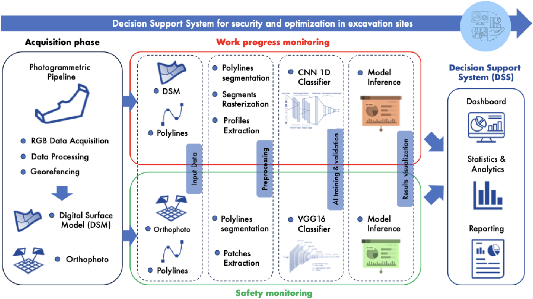
Overview of the proposed Decision Support System (DSS) for security and optimization in excavation sites. The workflow consists of three main phases: data acquisition, Deep Learning-based processing, and result visualization. The system performs two main monitoring tasks: work progress (red) and safety (green) monitoring. The results are integrated into the DSS, which provides a structured dashboard, analytics, and reporting tools to support decision-making in excavation site management.
During the acquisition phase, RGB images are captured through UAV flights. A key advantage of using RGB images instead of more advanced systems like LiDAR is the significantly reduced costs.7,8 Subsequently, the processing pipeline for orthophoto generation is initiated. Orthophotos are aerial photographs or satellite images that have undergone geometric correction, known as orthorectification. 9 The photogrammetric pipeline encompasses calibration, alignment, dense cloud generation, producing Digital Surface Model (DSM) data and orthophoto generation.
Given the diverse types of data available, we have identified two primary objectives: monitoring the progress of work and ensuring the security of an excavation area. For the first objective, the system must recognize and classify various work phases, including Closed Excavation (CE), Open Excavation (OE), and Pipe Laying (PL) areas (Figure 2).

Images of the work phases considered in this study: a) Closed Excavation (CE), b) Open Excavation (OE), and c) Pipe Laying (PL) areas of oil and gas construction sites. All the flights were performed with a DJI Phantom 4 RTK drone (d).
In this case, DSM data are utilized to evaluate excavation phases. For the second objective, the system aims to identify safety fences that define the perimeter of the excavation area from RGB orthophotos. To address these tasks, two different DL architectures are employed: a 1D (1-Dimensional) CNN for classifying work phases, 10 and a VGG16 network 11 for detecting the presence or absence of safety fences.
In the final step, the outputs from each network are integrated to drive a Decision Support System (DSS). This DSS automatically generates a report reflecting the updated status of the excavation area, encompassing both progress and safety aspects. This capability represents a significant practical advantage for human operators, as to our knowledge, existing literature lacks systems capable of autonomously producing reports to monitor both the status and safety of an excavation area. The combination of drones’ data acquisition, advanced analytics, and interactive reporting positions the DSS as an indispensable tool in modern construction management. It enhances efficiency and serves as a reliable source for decision-making, ultimately driving project success.
To summarize, the main contributions of the work are:
the collection and annotation of a real-world dataset from four different excavation areas, with multiple UAV flights per site to have data representing various stages of work progress; a novel pipeline integrating DL for monitoring progress and safety in excavation areas; the development of a container-based DSS that automates reporting and decision-making.
Real-time monitoring activities enable the automatic detection of work progress issues, anomalies, and hazardous situations.12–14 This process facilitates instantaneous and accurate assessment of ongoing activities, providing monitoring authorities with real-time data for timely decision-making and immediate action when necessary. 15
For data collection, two methods are typically employed: LiDAR and RGB photogrammetry. LiDAR maps complex terrains with dense vegetation cover, and it can detect small objects even in low-light or nighttime conditions. However, drawbacks include high cost, sensitivity to weather conditions like fog or rain, and limitations in capturing very small or thin details. Conversely, RGB sensors are widely available, more cost-effective, and still provide sufficient detail for a wide range of applications, particularly when combined with photogrammetry techniques. Photogrammetry is a low-cost way to produce high-resolution data, suitable for generating easily understandable maps and models (such as DSM) and detecting variations. 16 This process ensures precise measurement of true distances by providing an accurate representation of the Earth surface, correcting for factors such as topographic relief, lens distortion, and camera tilt. This capability is especially beneficial for the visual change detection task, aimed at precisely identifying differences between a reference (historical) image and a new test image depicting the current situation. 17 Moreover, RGB imaging allows the system to detect both geometric information and visual content such as colours and textures, enabling the dual functionality of progress monitoring and safety fencing detection in our use case. When dealing with images, challenges can become increasingly daunting due to variations induced by environmental factors, such as lighting conditions, weather patterns, and other environmental variables. These variations act as disturbances since the goal is to detect changes in images that are unrelated to these environmental factors. In addition, due to the distinct shooting angles of drones compared to traditional cameras, the accuracy in aerial photos is not optimal. 18 Numerous authors have conducted extensive research in this field. Some authors Chen et al., 19 and Ke et al. 20 have proposed algorithms that primarily focus on mitigating the effects of irregular motion in UAVs.
In recent years, DL algorithms, especially CNNs, are increasingly used in computer vision for quickly detecting and monitoring variations, with wide applications in civil engineering.21,22 In particular, CNNs23,24 are among the most widely adopted and effective tools in the monitoring context.18,25,26 For excavation area monitoring, the ability to automatically learn hierarchical features from images can be crucial for understanding the spatial relationships between different elements such as machinery, workers, and structures, 27 exhibiting robustness to variations in scale, orientation, and lighting conditions. 28 This is particularly important in this scenario, where the visual environment can be dynamic and diverse. 29 Moreover, CNNs can be updated or fine-tuned as the construction project progresses, 30 allowing for continuous learning and adaptation to evolving area conditions. This adaptability is valuable for addressing changes and optimizing monitoring strategies over time. 31
Recent advancements have also focused on integrating other AI techniques with CNNs to enhance fault detection and monitoring capabilities. For instance, a study by Kumar et al. 32 introduces a lightweight CNN model combined with an LSTM-AM framework to guide fault detection in fixed-wing UAVs, emphasizing the potential for improved performance and energy efficiency in edge-of-things applications. Additionally, several recent works have explored UAV-based monitoring for infrastructure assessment and excavation-related activities. In Pan et al., 33 the authors proposed a probabilistic deep reinforcement learning approach for optimal monitoring of buildings adjacent to excavation sites. This method highlights how advanced AI techniques can improve decision-making in excavation-related safety and monitoring tasks. Similarly, a knowledge distillation approach has been developed for recognizing excavation activities. 34 This work focuses on improving activity recognition in excavation sites, which aligns with the need for automatic classification of work phases in UAV-based monitoring systems. Other studies have investigated the role of UAVs in infrastructure inspection and intelligent route planning. In Pan et al., 35 the authors introduced a UAV-human collaboration model to optimize flight path planning for infrastructure inspection, demonstrating how UAVs can enhance efficiency and adaptability in monitoring workflows. Furthermore, a visual inspection and diagnosis system has been developed for detecting structural issues in bridge rivets using CNN-based methods, showcasing the increasing adoption of AI-driven UAV monitoring solutions in civil engineering. 36
While these studies demonstrate the growing impact of UAVs and DL in construction and excavation monitoring, our work uniquely focuses on integrating excavation phase classification and security fence detection into a single, automated DSS. This contributes to filling a research gap by combining UAV imagery with deep learning to support both progress tracking and safety compliance in excavation areas.
Materials and methods
This study develops an automated pipeline to enhance monitoring of work progress and safety in oil and gas excavation sites. The integration of drone technology facilitates the collection of aerial data, which is then processed using DL algorithms. This methodological approach not only automates data gathering and processing, but also enhances the analysis, enabling more accurate predictions of site conditions and potential hazards.
This section will detail the data collection, pre-processing stages and the specific DL algorithms employed for both the monitoring of work progress (Section 3.1) and safety fences (Section 3.2). Additionally, it will outline the data processing pipeline consisting of a container-based architecture for a serverless computing execution (Section 3.3).
Deep learning approach for work progress monitoring
In this section, the overall workflow for classifying the status of an excavation area is shown. Figure 3 illustrates a DL-based pipeline for processing UAV aerial images of excavation sites to determine their operational status using 1D CNN classification model on DSM data. The process consists of several steps:
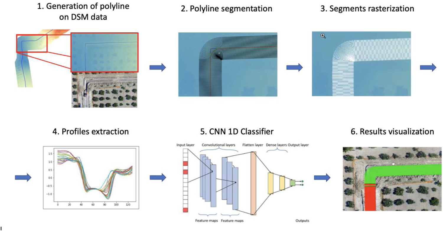
Overview of the deep learning-based pipeline for work progress monitoring. The process begins with the generation and projection of a georeferenced polyline onto DSM data, defining the excavation path. This is followed by segmentation into transversal segments, rasterization, and extraction of elevation profiles. These profiles serve as input for the 1D CNN classifier, which classifies excavation phases. The final output provides a visual representation of the classified excavation status for each segment.
the workflow begins with generating and projecting a polyline (imported as a georeferenced trace) onto DSM data, delineating the planned pipeline path based on project plans (Section 3.1.2). the polyline area is segmented into perpendicular sections, with a settable length and distance between each other (see Section 3.1.3). These elements will define all the cross-sectional areas (i.e. profiles) that will subsequently be classified by the model. the transversal segments are converted into a raster image, a grid of pixels, with lighter cells indicating the excavation area (Section 3.1.4). the cross-sections of the rasterized segments are extracted. These profiles represent variations in elevation across the excavation site, as extracted from the DSM (Section 3.1.5). a 1D CNN architecture is employed for classifying the status of the excavation profile over the three classes CE, OE, and PL (Section 3.1.6). the aerial image with areas colour-coded reflects the classifier’s output — in this case, green indicating segment profiles classified as OE while red for CE (Section 4.3.1).
In this study, three main work phases (classes) were considered to monitor the work progress (Figure 2). The first is closed excavation (CE), where the groundwork is laid out before any actual digging begins, ensuring that it follows the planned route, or where the trenches are backfilled once the pipes have been laid. Then, the project can proceed to the open excavation (OE) phase, where the actual digging of trenches occurs, followed by the pipe laying (PL) phase, where pipelines are physically installed into the ground. While these phases do not encompass all possible scenarios, they represent critical stages where tracking is essential for both project progress and safety compliance.
Aerial surveys at four Italian excavation sites (Gaeta, Caulonia, Benevento, and Balice) were conducted at heights of 30, 50, and 75 meters to optimise data acquisition. Flights at 100 meters were not employed in this study; instead, they were used to evaluate the suitable resolution in the data acquisition process: for instance, at this altitude, it was not feasible to discern the pipe laid in the excavation. All the flights were performed with a DJI Phantom 4 RTK. Flight paths were designed to maximize coverage of the excavation area while ensuring efficient data collection. The UAV follows a structured grid-based pattern based on georeferenced site maps and predefined waypoints. This systematic approach ensures that the acquired images provide a complete and consistent dataset for analysis.
At the Gaeta site, comprehensive data collection was achieved with 11 drone flights executed over time. This approach was essential for capturing the full spectrum of work phases, ensuring that each stage of excavation was thoroughly documented. The granularity of data obtained from Gaeta offers a temporal narrative of the site progression, from initial groundwork to the final stages of excavation. Balice site saw fewer flights (7) compared to Gaeta because the operations progressed more rapidly through the phases of interest to our study (and the monitored portion of the construction site was very small). In contrast, the sites at Caulonia and Benevento underwent fewer flights. Specifically, Caulonia was surveyed with 4 flights, while Benevento had 3 flights. This was due to the constraints of project schedules, which limited the opportunity to acquire data for the PL phase. Further information is given in Table 1. For each site, the distribution of extracted profiles for each work phase is reported. The profiles are generated according to the procedure outlined in the following sections.
Summary of drone flight data collection for excavation sites: Gaeta, caulonia, benevento, and balice.
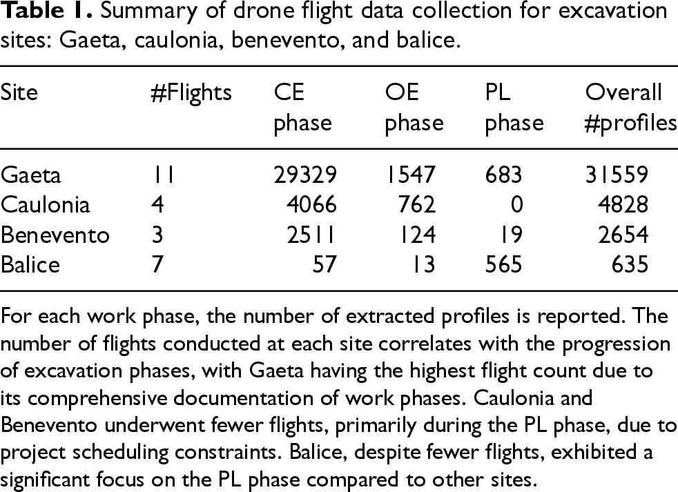
Summary of drone flight data collection for excavation sites: Gaeta, caulonia, benevento, and balice.
For each work phase, the number of extracted profiles is reported. The number of flights conducted at each site correlates with the progression of excavation phases, with Gaeta having the highest flight count due to its comprehensive documentation of work phases. Caulonia and Benevento underwent fewer flights, primarily during the PL phase, due to project scheduling constraints. Balice, despite fewer flights, exhibited a significant focus on the PL phase compared to other sites.
The orthophotos used have three RGB channels, saved in TIFF format. Each image is associated with a ”world file” with a TFW extension containing six lines of text, each representing a georeferencing parameter for raster images. These parameters constitute the coefficients of an affine transformation describing the position, scale, and rotation of the raster on the map. For example, if a raster image is shifted 10 meters east and 5 meters north, scaled by a factor of 1.2, and rotated 15 degrees, the transformation parameters encode these adjustments to align the image correctly in the mapping system. To ensure the correct visualization of the image with the appropriate projection, it is necessary to select the appropriate Reference System (RS) within the Geographic Information System (GIS) software. In the case of the orthophoto mentioned, the reference system is identified by the EPSG code 32633, also known as UTM33N, a standardized coordinate reference system used for geospatial mapping in central Europe.
The orthophotos include their corresponding DSMs, which have a single channel containing 32-bit floating-point data (see Figure 4). They are saved in a GeoTIFF file format that allows the incorporation of georeferencing information within the file itself. Information needed to establish the exact spatial reference for the file may include the map projection, coordinate system, and geodetic datum. The DSM is imported into QGIS software 37 with the same reference system as the orthophoto.
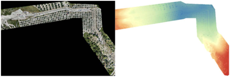
Images from QGIS software of the orthophoto (left) and the DSM (right). The DSM has a single-channel grayscale, but to better visualize elevation differences, a single-band “false colour” is employed.
The first necessary step involves the manual creation of a polyline, which is a sequence of connected segments forming a single object. This polyline is designed by the human operator to indicate areas earmarked for pipeline installation, according to project specifications. Using QGIS, an ESRI Shapefile (SHP file extension) was generated. Its geometry is of the LineString type, as discussed in the previous section. The orthophoto greatly facilitated the visualization of potential excavation areas and identified obstructions, such as vehicles and buildings. As shown in Figure 5, a notable challenge arises from the presence of a non-differentiable point, especially in regions where the polyline creates an approximate

Section of an excavation polyline, displayed in blue on QGIS software. The highlighted non-differentiable point represents a discontinuity in the excavation trajectory, which must be handled correctly to ensure accurate segmentation and profiling in the subsequent analysis.
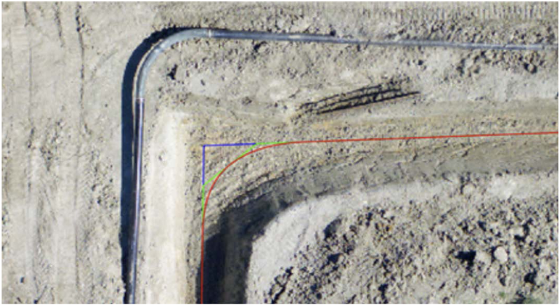
Image showing the original polyline (in blue), the interpolated polyline (in green), and the final polyline obtained from the Chaikin smoothing process (in red).
After establishing a singularity-free polyline, the subsequent objective was to generate a series of segments orthogonal to it. A sequence of points is generated along the path at intervals corresponding to the specified input distance. For each of these points, a longitudinal segment is created. The default values chosen for this process were a distance of 0.1 meters between segments (referred to as longitudinal ticks) and a segment length of 7 meters. These parameter values were determined through consultations and empirical testing with industry technicians. The 0.1-meter spacing was selected to ensure a sufficient density of sampling points without excessive computational overhead, while the 7-meter segment length was validated to balance spatial coverage and maintain alignment accuracy with real excavation features. Each segment is characterized by two attributes: a unique identifier code and the distance, measured in meters, from the starting point of the path (Figure 7).
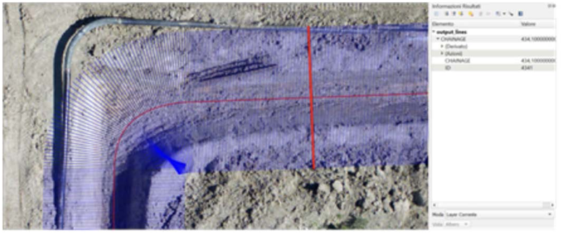
Segments are depicted in blue, while the polyline they intersect is shown in red. Specifically, the selected segment with an ID of 4341 is highlighted in red.
After completing the previous step, which involved generating segments perpendicular to the polyline, the subsequent task is to convert this vector data into raster format. During this phase, each transversal segment is assigned to a distinct gray-scale value, thereby imprinting these segments onto the raster image (Figure 8).
Screenshot from QGIS displaying two active layers. The base layer represents a portion of the DSM, visualized using a single-band false colour scheme to enhance elevation differences. The overlaying layer consists of rasterized segments, each assigned a distinct grayscale value, facilitating spatial analysis and classification.
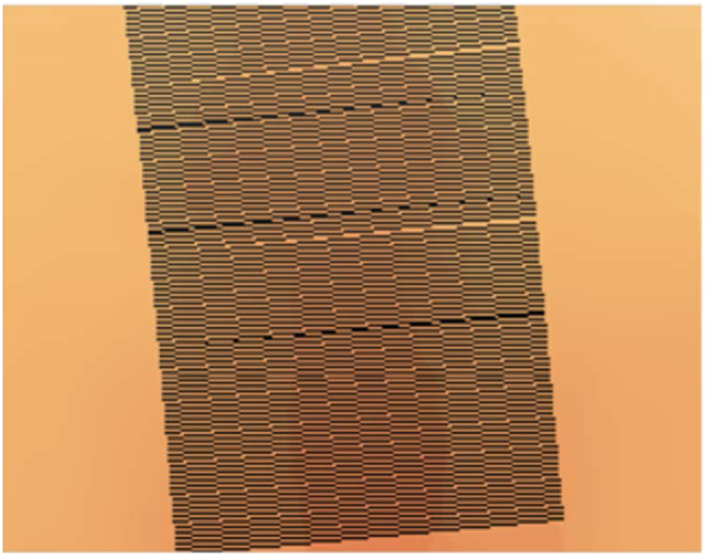
With an ordered dictionary containing all the Y-X coordinate pairs corresponding to the pixels of each rasterized segment, these coordinates are reported on the original DSM to derive the corresponding elevation values, or more precisely, surface values. In this process, original DSM data are subjected to an image smoothing step (specifically, a Gaussian blur with
Then, each profile requires appropriate labelling to generate a dataset suitable for the training phase of the CNN architecture. Specifically, concerning the elevation profiles, in this study labels can be categorized into ’0’ for CE, ’1’ for OE, and ’2’ for PL. Subsequently, an output JSON file is generated to encapsulate all elevation information of the profiles, along with the corresponding annotations.
Figure 9 shows an example of extracted profiles for each class. It is evident that the elevation range is greater for the OE and PL classes compared to CE. Furthermore, the distinction between OE and PL can be observed: in PL, the elevation range is reduced due to the presence of the pipeline inside, which is also discernible from the profile. However, the distinction between the two classes is not always clear-cut due to potential variations in the excavation depth and pipeline size, resulting in a similar overall shape. Additionally, noise from disturbances at the excavation site or generated during the acquisition procedure often contributes to this ambiguity. Figure 10 highlights the difference between clean profiles and profiles with noise.
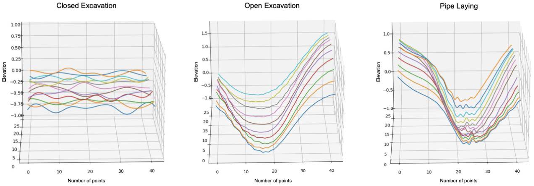
Some profiles of Closed Excavation (CE) (left), Open Excavation (OE) (center), and Pipe Laying (PL) (right) from flight #5 over the Gaeta site. CE represents sections where excavation has been completed or is yet to be opened, OE corresponds to active excavation areas with an open trench, and PL indicates sections where pipes have been placed inside the trench.
Example of OE profiles extracted from flight #5 over Gaeta site. The difference between clean profiles and profiles with noise is highlighted.
The DL architecture used to identify the status of the excavation area is a 1D CNN. 10 This architecture was selected due to its suitability for processing one-dimensional sequential data, such as time series or signals. In particular, 4 one-dimensional convolutional layers were used, including an input layer with a larger filter size compared to the subsequent layers to effectively capture more initial features. Following this, an average pooling layer was used, extracting average values from a specified grouping size, as it demonstrated superior empirical results compared to a classical Max pooling layer. Lastly, two layers of fully-connected neurones were implemented, where the first utilized a ReLU (Rectified Linear Activation Function) 39 as an activation function, and the subsequent and final layer employed a softmax activation function. The softmax function transforms a vector of K real numbers into a probability distribution with K possible outputs, 3 in this case. The architectural parameters of the network were validated through an ablation study to assess their impact on performance and ensure a balance between model complexity and accuracy.
Experimental procedure
For training the model, the optimization algorithm used was Adam. 40 A balanced sparse categorical cross-entropy was used as the loss function to minimize. This function sets the weights for each class in inverse proportion to the label frequencies in individual classes, partially addressing the class imbalance issue during the search for optimal model weights. For the selection of batch size, learning rate and number of epochs, it proved advantageous to use a low batch size, set at 8, with a learning rate of 0.001 for a total of 30 epochs. All hyperparameters were tuned in the separate validation set using a grid-search approach. Additionally, two classes of callbacks have been implemented into the model training: (i) EarlyStopping, which halts the training when the loss function value on the validation dataset begins to increase again, thereby limiting overfitting and reducing the required number of epochs; and (ii) ModelCheckpoint, which saves best model weights during training.
Considering the unbalanced nature of the dataset, two data augmentation technique were implemented to generate additional instances of minority classes:
SMOTE (Synthetic Minority Oversampling Technique),
41
that involves synthesizing new instances of minority classes. The process includes selecting neighbouring elements at homogeneous intervals, drawing lines between these elements, and introducing new samples along those lines. Flipping the training dataset: it entails reversing the order of profiles and labels relative to a vertical axis. By doubling the available data for model training, it contributes to a more diverse and robust training set.
To evaluate the generalization capability of the trained model, various splits of the collected dataset have been identified within three main distinct experimental settings:
Generalization on the same flight: 60% of the data from flight Generalization on other flights within the same construction site: data from flight Generalization across flights from different construction sites: data from flights on construction site X {
Generalization refers to the model’s capacity to categorize flight profiles based on specific criteria, such as the same flight, another flight, or another excavation area. The latter scenario, which is the most challenging, also happens to be the most intriguing as it reflects the practical application of the model (i.e., utilizing a previously trained model on a new excavation area). In all cases of dataset splitting, we have employed the stratification technique to ensure that each dataset faithfully mirrors the original distribution of classes.
In this section, the overall workflow for the safety task is shown. Figure 11 illustrates a DL-based pipeline for processing UAV aerial images of excavation sites to determine the presence of security fencing using VGG16 classification model on RGB images.
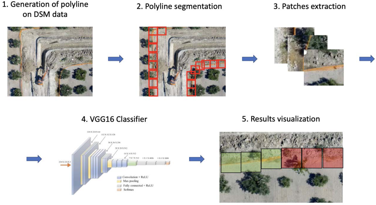
Overview of the deep learning-based pipeline for safety fencing monitoring. The process consists of a polyline manually or automatically defined along the excavation perimeter to delineate the expected safety fencing placement. Then, the defined polyline is divided into smaller segmented areas extracted from UAV-acquired orthophotos. Each patch is processed through a VGG16 classifier to determine the presence or absence of safety fencing. The final classification results are displayed, with different colours representing correctly fenced (green) and missing fencing (red) sections.
In this case, we consider RGB images rather than with DSM data, as safety fences are not detectable in DSM but are easily distinguishable in RGB images. The process consists of several steps:
the human operator generates polylines delineating the designated areas for fence placement (Section 3.2.2). the orthophoto is divided into smaller tiles with a settable dimension along the traced polylines (Section 3.2.2). individual tiles are extracted from the larger image for further processing. VGG16 Classifier: VGG16 CNN architecture is employed for classifying the tiles as ’No Fence’ or ’Fence’ (Section 3.2.3). the results of model classification are shown, representing areas with or without fencing by a colour-coded indication (Section 4.3.1).
The dataset used comprises same flights describe in Section 3.1.1. A total of 4608 for ’no fence’ and 5867 for ’fence’ patches were extracted from RGB orthophotos, according to the procedure described in next Section 3.2.2. The number of samples per class for each site are given in Table 2.
Summary of drone flight data collection for excavation sites: Gaeta, caulonia, benevento, and balice. The number of extracted patches for ’no fence’ and ’fence’ classes is reported.
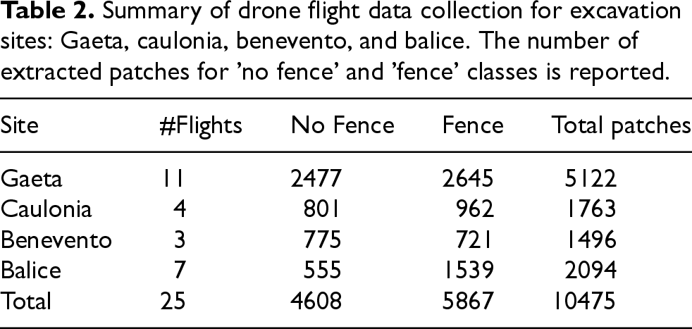
Summary of drone flight data collection for excavation sites: Gaeta, caulonia, benevento, and balice. The number of extracted patches for ’no fence’ and ’fence’ classes is reported.
Starting from the polyline delineating the intended placement of the fences, also in this case defined by the human operator and stored as an ESRI Shapefile, centres of the patches to be extracted are determined along its length at predefined intervals specified by the user. Next, the orthophoto is processed using the GDAL library (https://gdal.org/index.html), and the coordinates of the pixels and tile vertices are computed (Figure 12). The dimensions of the tiles can also be customized by the user; for our experiments, it was configured to
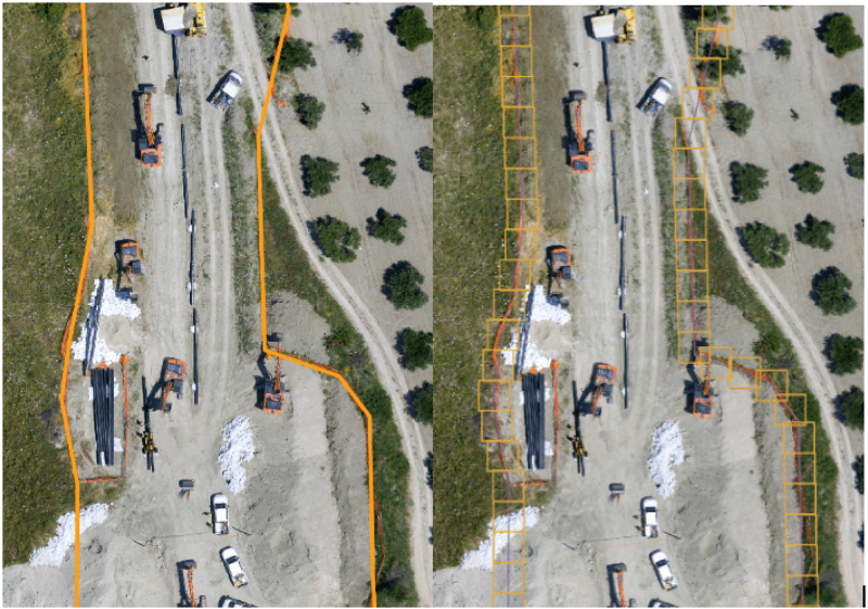
Representation of the polyline (left) and the extracted tiles (right) for the selected fencing.
The DL model employed is the VGG16 classifier,
11
a state-of-the-art CNN model for supervised image classification. The convolutional part of the architecture consists of 13 convolutional layers. Each of the 5 convolutional blocks has filters with a 3
Experimental procedure
The proposed model was compared with other state-of-the-art CNN architectures for image classification, namely AlexNet 42 and ResNet18. 43 These models were selected for two key reasons: (i) their competitive performance in the ImageNet challenge, and (ii) their relatively simple design (i.e., not too deep), which facilitates the extraction of low-level features for fine-tuning. AlexNet was included as a computationally efficient baseline with respect to VGG16, while ResNet18, with its residual connections, enhances feature extraction and is particularly effective in distinguishing subtle variations, like in excavation site structures. Additionally, a more complex vision transformer architecture, the Swin Transformer, 44 was also employed. Its hierarchical structure allows it to process images at multiple scales, i.e. (H/4, W/4), (H/8, W/8), (H/16, W/16), and (H/32, W/32), progressively capturing both fine-grained details and broader spatial context.
A transfer learning approach was utilized to fine-tune the networks, leveraging pre-trained weights from ImageNet. 45 While the selected models leverage pre-trained weights, our dataset differs as it focuses on UAV-based excavation imagery with large-scale terrain features and almost uniform textures. However, it is well established that transfer learning provides significant benefits, as low-level features such as edges and textures are transferable, while higher-level features require fine-tuning for domain adaptation. For the VGG16 architecture, all layers were frozen except for the last four convolutional layers.
We used a mini-batch stochastic gradient descent (SGD) optimizer and explored optimal hyperparameters, including batch size, initial learning rate, and momentum, within the ranges {32, 64, 128}, {1
Data processing pipeline
A pipeline based on Amazon Web Services (AWS) and Docker containers has been developed to support both work progress monitoring and safety monitoring tasks in excavation areas. This system consists of multiple interconnected modules, each responsible for a specific function in the workflow.
The work progress monitoring pipeline (Figure 13) follows a structured three-step process:
Segmentation Module: the process starts with an API Gateway request triggering a Lambda function, which downloads the excavation polyline shapefile from Amazon S3. The polyline is then segmented into smaller parts, which are stored in the segment table, while the complete segmented polyline is saved in the shapefile table. Preprocessing Module: in this phase, the DSM file is retrieved, and the segmented polylines are rasterized to align with the DSM data. The processed profiles are converted into JSON format and stored in Amazon S3, with their metadata recorded in the profiles table in a PostgreSQL database. Inference Module: the preprocessed profiles are then passed to the DL inference module, where a trained DL model classifies the excavation phase for each segment. The predicted class is saved in the results table, and the outputs are formatted for visualization in QGIS, facilitating real-time tracking of excavation progress.
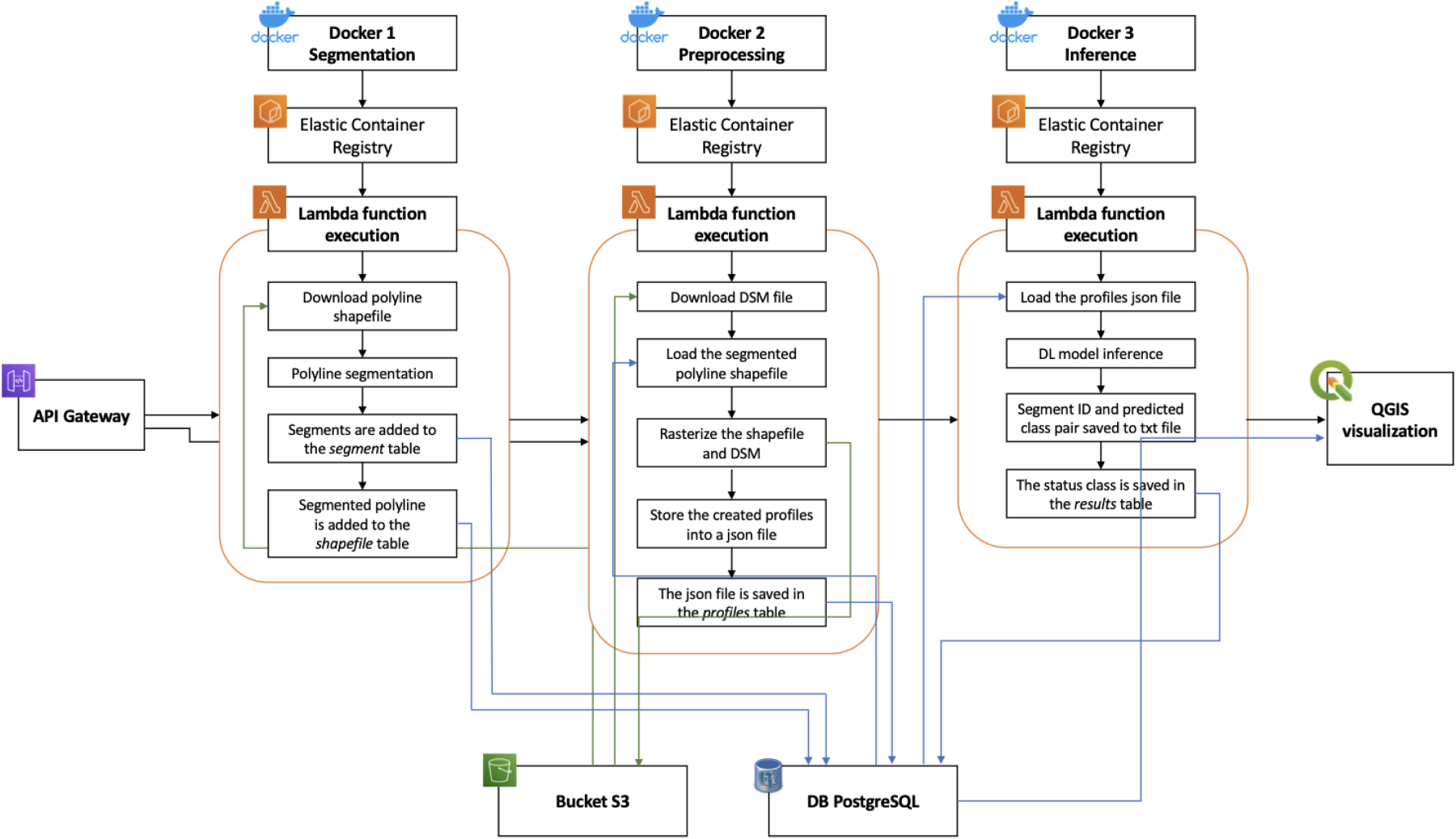
Data processing pipeline for work progress monitoring task.
The safety fencing monitoring pipeline (Figure 14), while similar in its use of AWS and Docker-based processing, is structured as a single dedicated module focused on detecting safety compliance using DL. This module follows a comparable approach, where UAV imagery is processed through a segmentation, classification, and visualization workflow to assess the presence of safety fencing along the excavation perimeter.
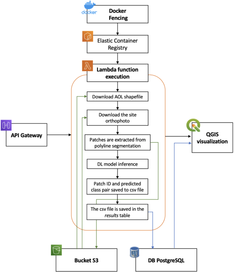
Data processing pipeline for safety monitoring task.
Each module is encapsulated within Docker containers, ensuring portability and scalability. The workflow begins with Docker images uploaded to Amazon Elastic Container Registry (ECR), which are then processed using AWS Lambda functions. These functions execute the code on demand, automatically scaling based on processing needs. The integration of API Gateway allows external services to invoke specific modules via REST APIs.
The collected data and the results from these processing methods are seamlessly integrated into a digital platform with repository, management, and reporting functionalities for excavation area activities (see Section 4.3). This platform operates within a georeferenced environment, creating a comprehensive and universal system that encompasses various stages. Through this approach, companies in the oil and gas sector achieve automated control over diverse processing steps and enhance site safety, all while improving collaboration with requesting organizations, such as public entities.
Results of the work progress monitoring
Throughout the experimental phase, we performed various tests to validate the accuracy of the proposed model. In this context, the evaluation of the model generalization on flights from another excavation area is the most crucial for assessing the model’s reliability, even if the most challenging scenario.
Generalization on the same flight
For this test, flight 5 of Gaeta site was considered, as it provided relatively sufficient samples across all three classes of interest, with the following distributions across 2869 total profiles: 2403 CE, 364 OE, and 102 PL. For the test set, 20% of the data was considered, split in a stratified manner. From the confusion matrix in Figure 15(a), the results obtained reveal 557 profiles correctly identified against 17 misclassified profiles out of a total of 574, resulting in 97% accuracy. The results of all metrics are shown in Table 3.

Confusion matrices showing model performance in Gaeta site flights. (a) 20% of Flight 5 as test set and (b) Flight 8 profiles as test set.
Summary of performance metrics (accuracy, precision, recall, F1-score) of the work progress monitoring classification model under different generalization scenarios: (i) the same flight used for training, (ii) other flights from the same excavation area, and (iii) flights from a different excavation area.
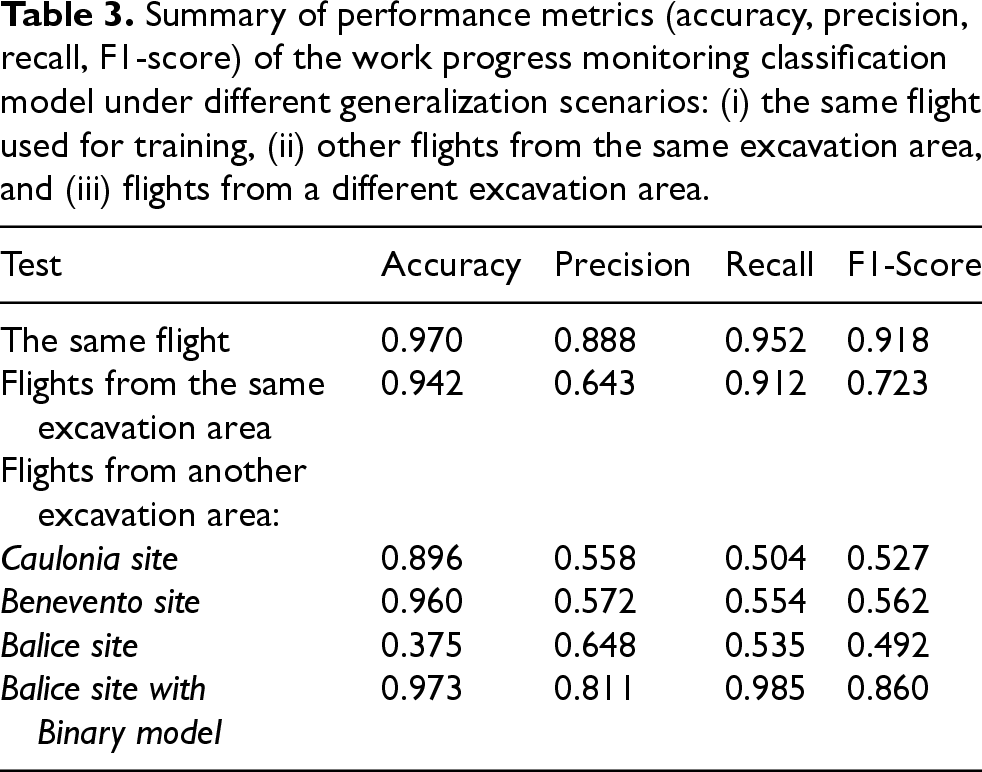
For this test, data extracted from all flights in Gaeta were considered as training and validation sets, excluding flight 8, which was used as the test set. The results obtained reveal 2692 profiles correctly identified against 167 misclassified profiles, out of a total of 2859 profiles (Figure 15(b)). This corresponds to a model accuracy of 94% in predicting profiles on a new flight from the same excavation site on which it was trained. The results of all the other metrics are shown in Table 3. One crucial aspect to consider in evaluating the model’s performance is the dataset balance. Class CE has significantly more examples compared to the other classes, indicating a high level of imbalance. However, the model demonstrated a good degree of accuracy in all the classes, PL as well, even if there are few false negatives with respect to OE.
Generalization on flights from another excavation area
Test on Caulonia site: For this test, data extracted from all flights in Gaeta and Balice were used as training set, Benevento flights as validation sets, and Caulonia flights were used as the test set. The results obtained include 4326 profiles correctly identified versus 502 incorrect profiles, out of a total of 4828 profiles (as shown in Figure 16). This corresponds to an 89% accuracy of the model in predicting data from flights of another excavation area compared to the one it was trained on. However, the predominance of samples in the CE class significantly influences the accuracy evaluation of the model. Classes with fewer examples are not accurately represented due to this class imbalance. Moreover, the model erroneously predicted instances as belonging to the PL class, despite the absence of any examples of this class in the ground-truth data.
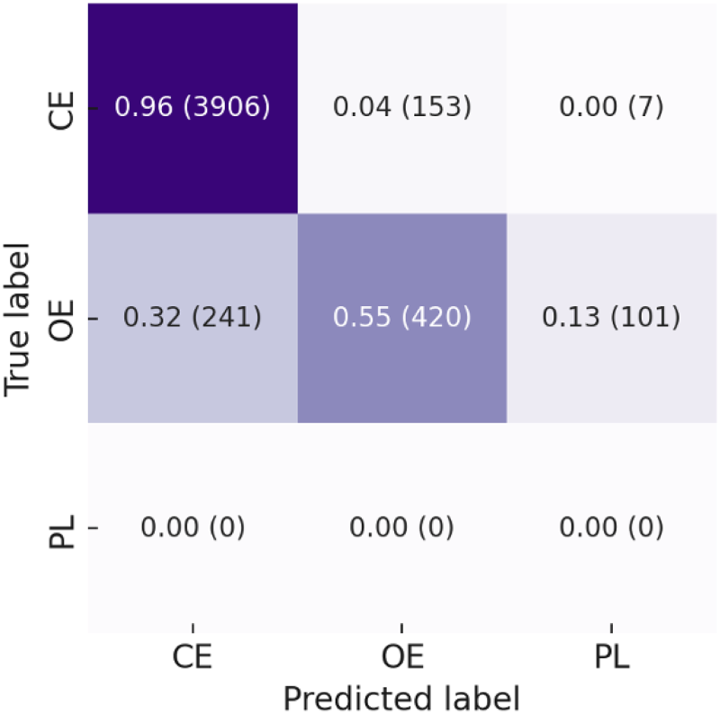
Confusion matrix showing model performance in Caulonia flights as test set.
Test on Benevento site: Since there were no PL profiles in Caulonia to test the model’s generalization in all classes, flights from Benevento excavation area were used as a test set. For this test, data extracted from all flights in Gaeta and Balice were used as training set, Caulonia as validation set and Benevento flights were used as the test set. From the analysis of the confusion matrix (Figure 17), it is evident that the performance for the CE and OE classes aligns proportionally with that observed in Caulonia. Concerning the PL class, only 3 out of 19 profiles are correctly classified, indicating a challenge in distinguishing these profiles from those in the OE class. The similarity in profile shapes suggests that the elevation differences, which differentiate between OE and PL, might be less pronounced in certain excavation areas, such as Benevento, compared to others like Gaeta (see Figure 18). Moreover, the limited number and diversity of training data may hinder the model’s ability to generalize accurately to profiles from different excavation areas. Notably, the absence of the inner tube profile in the training data and variations in elevation differences between OE and PL across different areas contribute to classification difficulties. Furthermore, the discriminative elevation differences observed in Gaeta may not hold true in other excavation areas without model re-training. This discrepancy could be linked to variations in actual flight elevation, further complicating the classification task. However, the model does not require full re-training for each new site; a single annotated flight containing representative excavation phases is typically sufficient for fine-tuning and local adaptation.
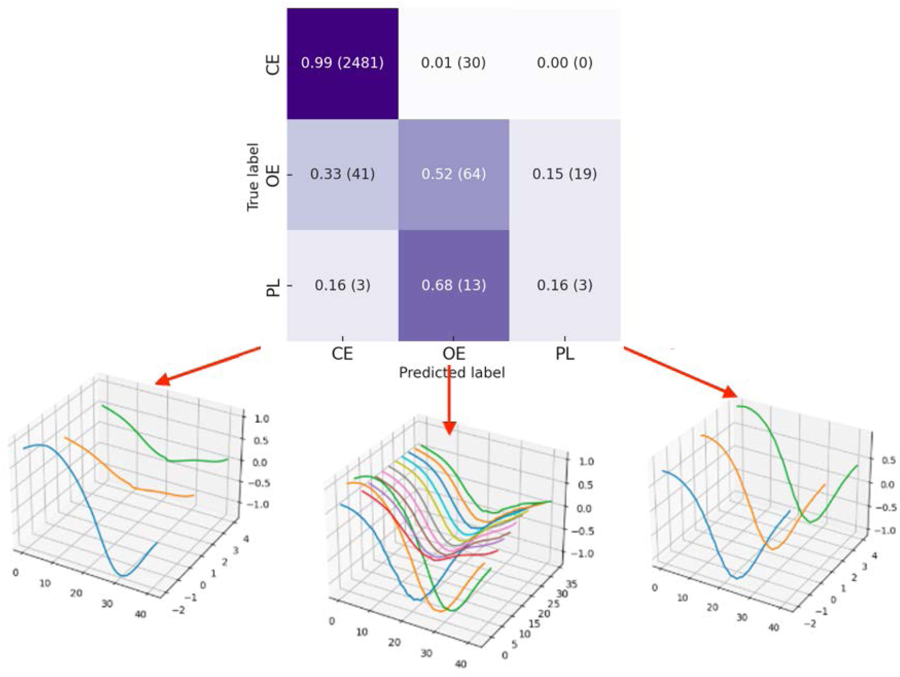
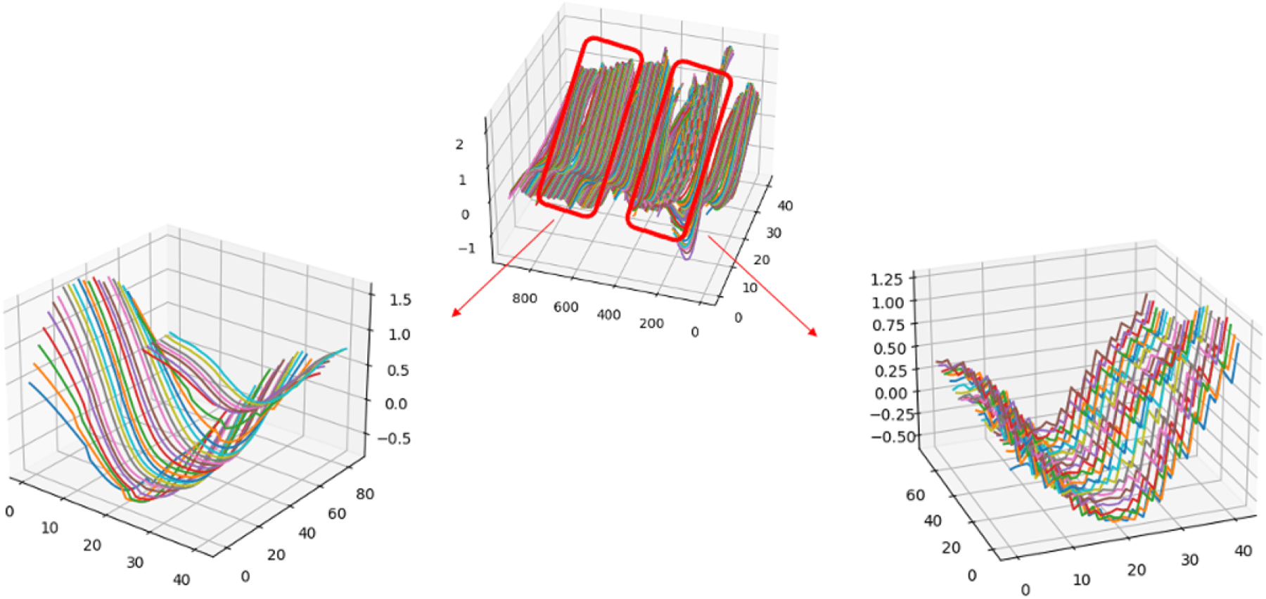
Confusion matrix showing model performance in Benevento flights as test set (class ’0’ is CE, class ’1’ is OE, class ’2’ is PL). Below, a detailed plot of the correctly classified profiles (right) and the incorrect ones.
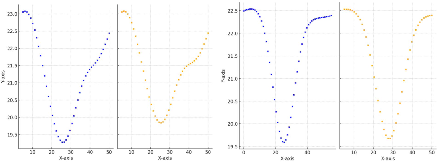
Examples of OE (blue) and PL (orange) profiles obtained from a Gaeta flight at 75 m (left) and a Benevento flight at 75 m (right). Notably, there is a distinct difference in the patterns between the two excavation areas. In Gaeta, the difference between minimum points of OE and PL profiles is 0.56 m, while in Benevento, this difference is reduced to 0.11 m. This discrepancy underscores the variability in profile shapes across different excavation sites, highlighting the challenges in accurately classifying the OE and PL phases.
Test on Balice site: Since the analysis of the PL phase profiles often reveals only a decrease in elevation compared to the same excavation without a pipe, due to the interpolation of the DSM, this phenomenon can nevertheless serve as a criterion for classification. Consequently, a two-stage solution was implemented. As a first step, a binary classification model is employed to classify only CE and OE phases. Subsequently, a post-processing step is required, involving a ’rule’ that assesses the elevation difference of the classified OE profiles between the previous and current flight: if the difference exceeds a certain threshold defined empirically by the company based on the cross-sectional area of the pipe, the profile is classified as PL. Upon comparing the results in Table 3 obtained from the model trained directly with the three classes against the binary classification combined with the post-processing approach, it becomes evident that the latter methodology resolves nearly all the confounds of the model, achieving a 97% accuracy (Figure 19).

Comparison between the results obtained with a) one-stage model and b) two-stage solution on Balice test set. (a) Results of the three classes model (CE, OE, PL) and (b) Results of the binary model (CE, OE) combined with post-processing for discriminating OE-PL classes.
For this experiment, the dataset was split with 80% images for training and the remaining 20% for testing, following a hold-out criteria at site-level. Specifically, Balice flights (with different qualities of light conditions and terrain) were designated for the testing phase. This approach was adopted to assess the algorithm’s generalization ability under diverse environmental conditions. Additionally, 20% of the training data was further divided into a validation set to identify the optimal hyperparameters for the model.
Classification performance
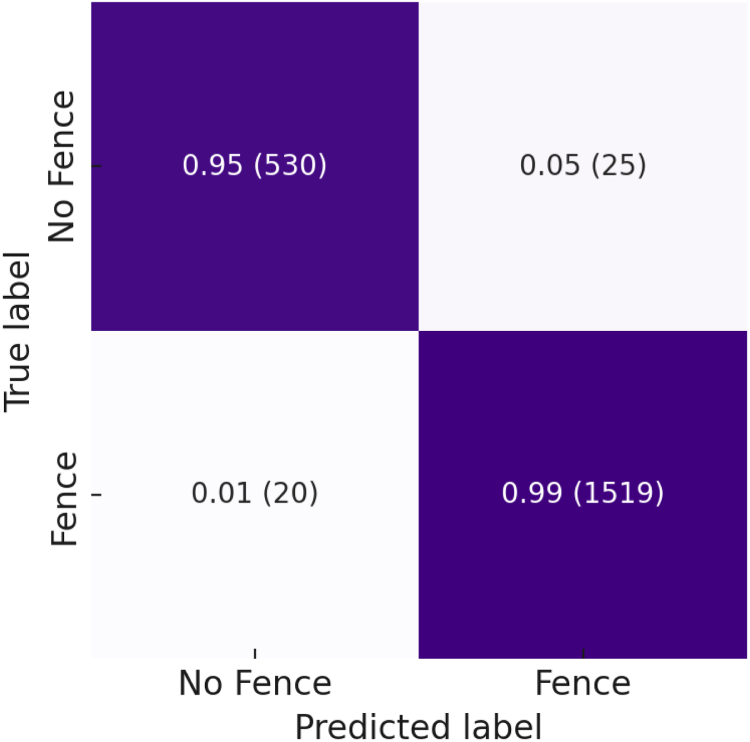
Table 4 displays the classification performance of VGG16, ResNet18, AlexNet, and SwinTransformer on the test set for solving the fencing classification task. VGG16 outperforms all other state-of-the-art models in terms of Accuracy, Recall, Precision, and F1 score. Additionally, analysis of the confusion matrix depicted in Figure 20 reveals:
the model misclassifies 25 ’No Fence images as ’Fence’. However, in reality, a fence is present in 24 out of 25 of these photos. Therefore, the algorithm correctly identifies samples that were annotated incorrectly; the model incorrectly labels 20 ‘Fence’ images as ‘No Fence’. Yet, in reality, there is no fence present in only 12 out of 20 of these photos; out of the total misclassified images - which include erroneously annotated ones - 36 out of 45 errors (80%) are observed. Hence, the algorithm effectively makes only 9 errors, suggesting that the accuracy could be even higher than the reported 98% mentioned earlier.
To further validate the statistical significance of our results, we conducted an ANOVA test (F-statistic
To conduct a more detailed analysis of the model’s errors, the Grad-CAM technique was employed, 46 which provides an activation map highlighting the relevant regions of the image for class prediction, offering a visual ’explanation’ of the classification process. From the visual results below (Figure 21), it can be observed that out of the total 45 errors made by the model, as reported in the confusion matrix, only 9 appear to be actual misclassifications. For instance, in images labelled as ’No Fence’, most cases indeed feature a ’Fence’ as predicted by the model. In other instances, there are still orange elements, not clearly identifiable as a ’Fence’ or something else, on which the CNN focuses and thus predicts as ’Fence’. We chose to assess the performance of the model on the original dataset, including its annotation errors, to evaluate the difficulty of the task and to demonstrate that the model is robust even when the human expert fails.
Classification performance of VGG16, resNet18, alexNet and swinTransformer for solving fencing classification task. Inference time (IF) is computed as seconds per image.

Classification performance of VGG16, resNet18, alexNet and swinTransformer for solving fencing classification task. Inference time (IF) is computed as seconds per image.
Results related to Balice flights for fencing monitoring.
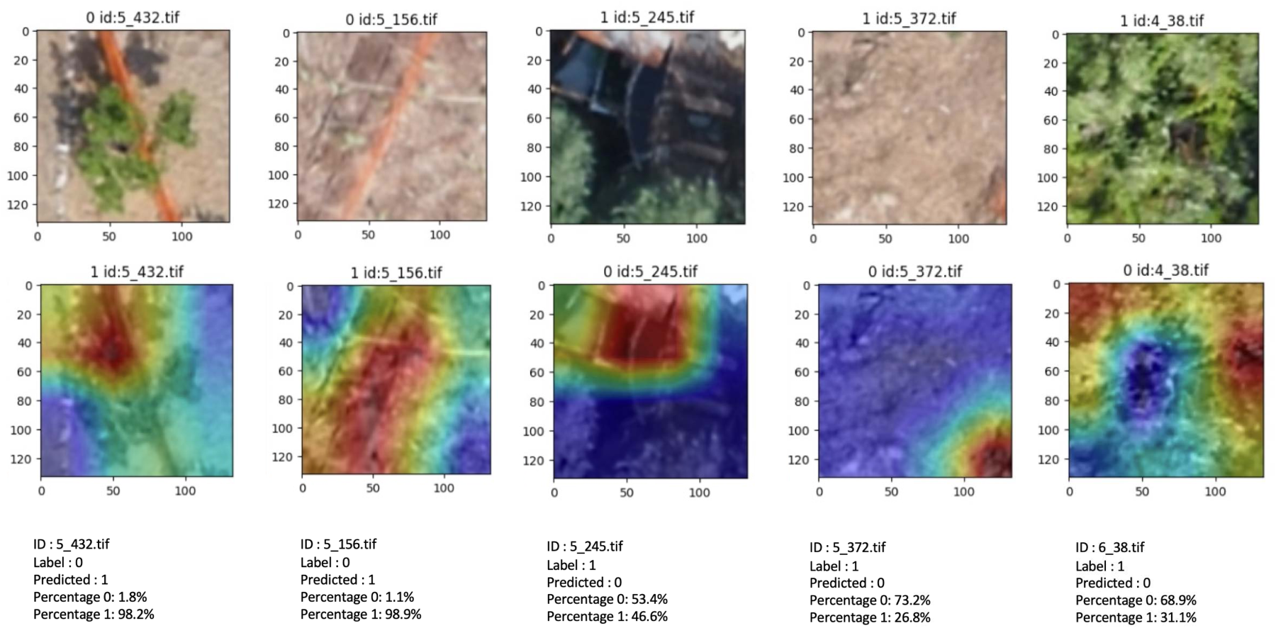
Some examples of the application of Grad-CAM for Model Error Analysis. This visualization uses the Grad–CAM technique to highlight areas in the images that influenced the model’s predictions, thereby providing insight into the classification decisions. Class ’0’ indicates ’No Fence’, class ’1’ is ’Fence’; ’Label’ is for ground-truth annotation, ’Predicted’ is the model inference. It is possible to notice that sometimes annotations - performed in automatic way - are wrong (first three images from the left). In other cases, the setting is very challenging, leading to incorrect ’No Fence’ predictions as in the last two images.
The final DSS is equipped with a rich dashboard that serves as the command centre, providing stakeholders and project managers with a comprehensive overview of the project progress and vital metrics. The core of the DSS dashboard is designed for ease of use, offering a user-friendly interface that allows for real-time monitoring of various excavation area activities. As depicted in Figure 22(a), the dashboard leverages orthophotos from drones to present a high-resolution visualization of the excavation area. Moreover, a key feature is showcased: a dynamic temporal slider that enables users to conduct a visual comparison between two different drone flights over the same excavation area, captured at distinct time intervals. This comparative function is essential for monitoring the progression in the site and the various phases detected by the DL model over time, as well as for identifying any changes made or potential anomalies observed.
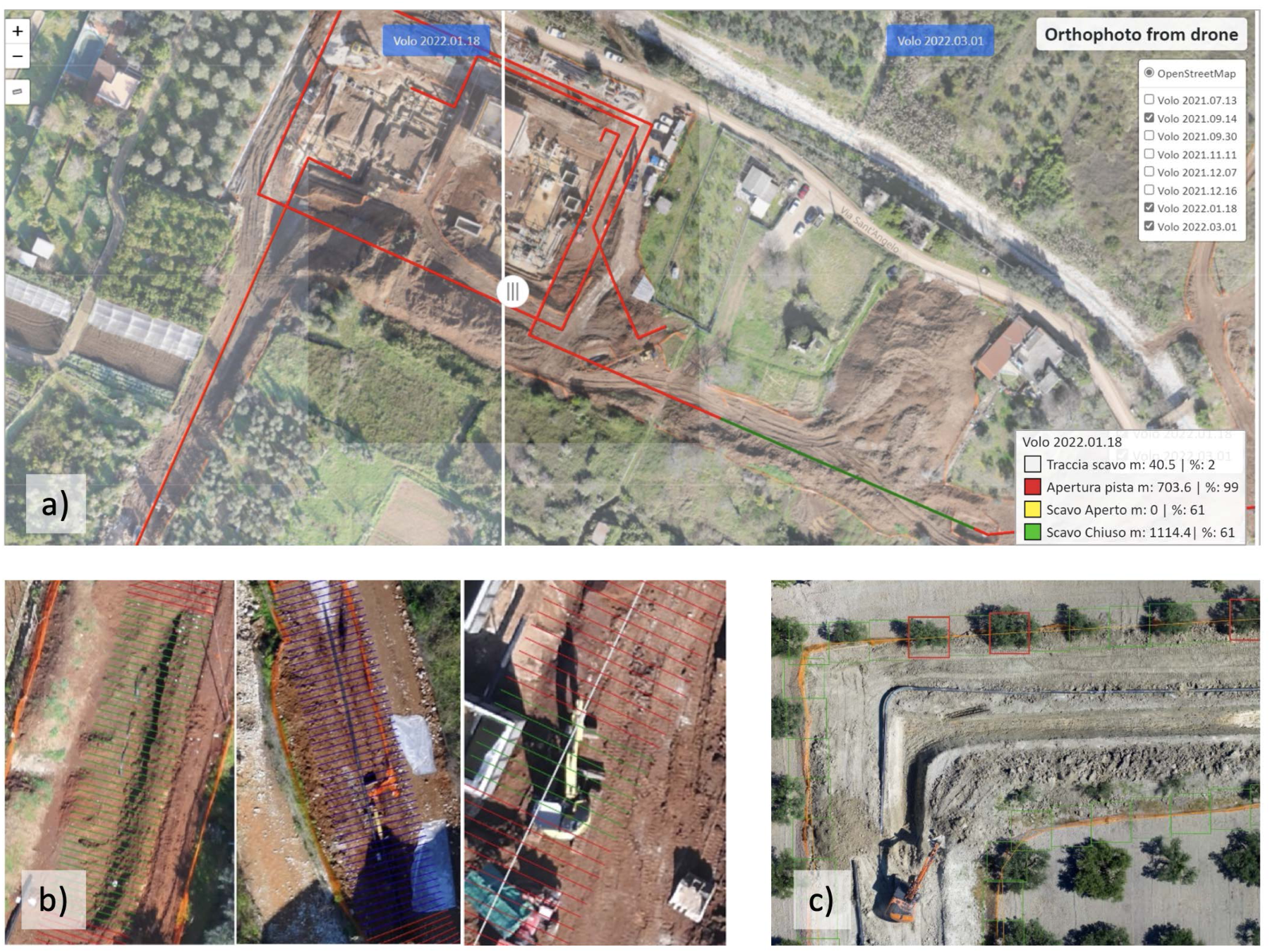
a) Visualization of the model predictions across the entire excavation area, with the comparison of different drone flights; b) Example of correct classification of OE (left); Example of correct classification of PL (center); Example of incorrect classification due to the presence of a heavy vehicle (right); c) Visualization of the network inference results: green patches indicate the presence of a fence, while red patches indicate no fence.
For the work progress monitoring, the interface displays the model predictions highlighting the different classes with colour-coded indicators, i.e. CE in red, OE in green, and PL in blue (Figure 22(b)). Results are displayed through communication with the QGIS software, by means of two operations facilitated by the programme through the properties of each layer:
Union of a layer with a data source: this involves merging the output-lines layer, containing all profiles, with the file generated by the predictions of the DL algorithm. This union is carried out through the ‘ID’ parameter. Symbolization of the data derived from the join, particularly from the ’LABEL’ parameter in the file. It focuses mainly on categories such as CE, OE, and PL.
As regards the safety monitoring, the coloured patches indicate areas where the VGG16 classifier has inferred the presence or absence of the fence network: green patches signify the presence of a fence, while red patches indicate areas with no fence, enabling a quick visual assessment of perimeter security (Figure 22(c)). Importantly, each patch is georeferenced, allowing the operator to precisely locate the area on the map. This enables efficient planning of on-site inspections, particularly for patches flagged as ”no fence”. These can then be validated by the operator to verify whether fencing is actually missing or simply occluded (e.g., by a tree or equipment). The integration of georeferenced outputs into QGIS thus ensures that both progress and safety assessments are spatially contextualized and easily actionable by field personnel.
Reporting is streamlined within the DSS, with the ability to automatically generate detailed reports that include progress monitoring as part of the site management process. These reports are structured to present clear and actionable insights, with percentages indicating the progress status for different site sections, as illustrated in Figure 23. This includes the comparison of planned versus actual progress, empowering the project management team to track milestones and adjust workflows as necessary. This automatic report generation module ensures that project stakeholders receive real-time, data-driven insights without requiring constant manual supervision. This structured information flow enhances decision-making efficiency by providing a clear overview of project progress and compliance, supporting timely and informed interventions where necessary.

Dashboard for project progress monitoring: on the left box, bar charts illustrating the comparative progress status for specific area segments. The light blue bars represent the planned progress percentage for each project phase, while the orange bars indicate the actual completion percentage as monitored on the reported date. This visual representation serves as a report from the DSS, providing an at-a-glance confirmation of project adherence to planned timelines and swift identification of areas requiring focused attention.
Considering the task of work progress monitoring, it is evident that deep DL models demonstrate high performance when applied to data resembling the training set, such as data from the same flight or flights within the same excavation site. However, challenges arise in generalizing the model performance to data from different excavation areas, particularly concerning the PL class. This underscores the necessity for a more diverse dataset during training to improve model generalization. Despite these challenges, the three-class model (CE, OE, and PL) excels in distinguishing between CE and OE. Although accurately identifying the PL class proves challenging, especially due to potential inaccuracies in DSM capturing, specialized post-processing techniques effectively mitigate confusion with the OE class. A significant factor impeding the training of individual models is the uneven distribution of the classes, with a notable abundance of the CE label compared to the other two. Moreover, the profile characteristics of these labels vary considerably based on the excavation area and flight altitude. Another critical issue is the unreliable capture of the PL in the DSM, which leads to its loss during point cloud interpolation. This complexity hampers the ability of the DL model to differentiate between OE and PL. It should be interesting to consider LiDAR sensors mounted onboard of UAV to improve the quality of derived DSM with a higher density of points over the monitored area. Regarding the safety task on fencing monitoring, the results obtained from the analyzed dataset are promising. The distinctive colour feature and network geometry render the task manageable for robust models like VGG16. However, the relative similarity among available images may hinder a comprehensive evaluation of the algorithm robustness. Variations in illumination and shading can impact model performance, while differences in image resolution and input signal quality may affect inference accuracy. Additionally, similarities in texture or colour between the fence and surrounding terrain pose challenges for the classifier in accurately discerning areas with and without a fence. The integration of automated report generation into construction monitoring workflows contributes to improved situational awareness and decision-making. By reducing reliance on manual assessments, the system minimizes human error and facilitates proactive issue resolution. While currently focused on monitoring and reporting, future developments could explore extending the system toward more decision-support functionalities, such as predictive analytics for project delays or real-time alerts for safety non-compliance.
Conclusions
This paper presents a workflow designed to automate the monitoring of excavation area progress and fencing presence using advanced DL methods. The approach not only tracks these elements but also generates detailed real-time reports, enhancing efficiency, accuracy, and safety in project management. Our approach is novel in integrating a DSS for excavation monitoring, representing a key advancement in project safety and management. The system aligns with EU-OSHA’s ”Safety and Health at Work in the Digital Age” campaign, contributing to workplace safety in excavation areas (https://osha.europa.eu/it). By integrating digital technologies and innovative approaches to ensure workplace safety, our proposed system resonates with the objectives of this campaign, contributing to the advancement of safety in the excavation areas. A key strength of our approach is its adaptability to various deep learning techniques. While our experiments primarily focused on specific DL models, the framework is designed to remain flexible and not constrained to a single deep learning paradigm. This adaptability allows for the integration of alternative architectures, such as other recurrent models or Transformers architectures, which could be explored in future research. Future work may include monitoring additional phases like pipe welding, even using alternative acquisition methodologies such as LiDAR or Airborne Laser Scanning (ALS) for improved terrain profiling and classification accuracy. Additionally, integrating multi-spectral imaging could enhance our approach by capturing material variations, temperature changes, and improving visibility in low-light conditions. This would strengthen safety monitoring and anomaly detection in excavation sites. Future research will explore the integration of multi-spectral data through multimodal DL approaches, enabling the fusion of RGB, thermal, and other spectral modalities to improve classification. Finally, a continuous learning approach could also enhance model performance by incorporating feedback and corrected classification errors. In addition to construction site management, another promising application of our approach could be the monitoring of manufacturing production stages, enabling real-time tracking of production processes. Future research will explore how our methodology can be adapted to industrial manufacturing environments, leveraging automation and AI-driven insights to enhance operational performance. Furthermore, other advanced machine learning approaches, such as Dynamic Ensemble Learning 47 and Finite Element Machine 48 could be explored to improve model adaptability, computational efficiency, and robustness in dynamic environments.
Footnotes
Funding
The authors disclosed receipt of the following financial support for the research, authorship, and/or publication of this article: this work was supported within the research agreement between Università Politecnica delle Marche, Techfem Spa, and Sinergia EPC Srl.
Declaration of Conflicting Interest
The authors declared no potential conflicts of interest with respect to the research, authorship, and/or publication of this article