
Abstract
As large-scale collaborative, cross-cultural ethnographic research becomes easier and easier to realize, certain ethnographic methods and analyses should be correspondingly more available, inviting, and accommodating. We have therefore created AnthroTools, a package for the free, open-source language R, with a variety of tools and functions suitable for both multi-factor free-list analysis and Bayesian cultural consensus modeling. Free-list data elicitation is a simple technique for ethnographic research. However, especially for cross-cultural free-list data, background preparation is considerable and often requires specific software. In addition, although current cultural consensus analysis tools offer very sophisticated analyses, they also either require specialized software or have computationally taxing methods. AnthroTools expedites these techniques, rapidly performs diagnostics, and prepares data for further analysis. In this article, we briefly discuss what this package offers cross-cultural researchers and provide basic examples of some of its functions.
Introduction
Analytical tools in cultural research often suffer from the need for a considerable amount of processing, cleaning, and preparation before analyses. Although extant free software such as ANTHROPAC/UCINET (Borgatti, 1996; ANTHROPAC henceforth) is ready-made for consensus and content domain analyses, such software often requires data to be organized in ways not suitable for integration with greater data sets and requires navigating software-specific interfaces that are not readily transferable to other programs. Because of this, we created AnthroTools (Jamieson-Lane & Purzycki, 2016), a simple package for use in R (R Core Team, 2012) to facilitate data management and analysis for social scientists interested in cross-cultural research. Currently, AnthroTools is equipped with two primary modes of analysis: (a) free-list data analysis and (b) cultural consensus analysis, both of which are foundational for cross-cultural and ethnographic research (see Bernard, 2011; Handwerker, 2001). In this article, we introduce the theory and practice of both methods of analysis, discuss AnthroTools in the context of other tools currently available, and provide walkthrough examples of the package’s utility to perform said analyses. We refer readers to the package’s help menu (run
Free-List Tasks
Free-list data elicitation techniques are invaluable for assessing the content and structure of explicit human thought (Gravlee, 1988; Quinlan, 2005; Romney & D’Andrade, 1964; Schrauf & Sanchez, 2008; Smith, 1993; Smith & Borgatti, 1997; Smith, Furbee, Maynard, Quick, & Ross, 1995; Thompson & Juan, 2006). Free-list tasks generate data that—when appropriately analyzed—readily approximate our mental models of any given domain. Shared models and their content are “cultural models” (D’Andrade, 1981; Goodenough, 1957).
In these tasks, participants list objects in a given domain. At its core, the task lends itself to accounting for the ubiquity of specific items, but also to concept salience (i.e., its cognitive accessibility and/or importance; see below) across the minds of individuals. There are also many other useful accompanying methods to free-listing such as ranking, evaluation, and sorting (Brewer, 2002). Free-lists are useful as a preliminary step toward more focused research efforts such as scale designs and pile sorting (Bernard, 2011; Brewer, 2002; Handwerker, 2001). Moreover, the presence, absence, or co-occurrence of listed items, item frequencies, and/or salience scores may also be used as dependent or independent variables in targeted studies (e.g., Purzycki, 2016; Schrauf & Sanchez, 2008) and thus may serve as an end in themselves.
Researchers have regularly used free-lists for nearly half a century. Some domains of inquiry using this technique have been the animals people know (Henley, 1969), color terms in English (Smith et al., 1995) and Estonian (Sutrop, 2001), wildflowers (Robbins & Nolan, 1997), plants that treat intestinal worms (M. B. Quinlan, Quinlan, & Nolan, 2002), things that people need to live a good life (Dressler, Borges, Balieiro, & dos Santos, 2005), the kinds of fruits they know (Bernard & Ryan, 2009; Hough & Ferraris, 2010), things that people think gods like and dislike (Purzycki, 2011, 2016; Purzycki et al., 2016), dishes of food across social classes in Argentina (Libertino, Ferraris, Osornio, & Hough, 2012), models of what constitutes good or bad people (Purzycki, 2016), and many, many others.
Free-list tasks are quite simple to execute, and provided that questions are relevant, they are virtually effortless for participants from all walks of life to answer. Researchers can limit the number of items listed, or ask participants to exhaust their available knowledge. In addition to responses, recording the order in which participants offer them is also important, as it lends itself to calculating cognitive salience or the accessibility of specific items. Items listed earlier are typically more salient and often more ubiquitous within a sample (Romney & D’Andrade, 1964). As discussed below, free-list data do require more backend processing than, for instance, scale-based quantitative data. However, the task has the benefits of not requiring forced responses (a common concern), it is a naturalistic method and easy for samples who have difficulty with scales, and it is quite easy to recode data using whatever scheme a researcher wishes to use thus facilitating cross-cultural comparison. The task is therefore ideal for navigating the relationship between emic and etic models of cultural information (Harris, 1976; Headland, Pike, & Harris, 1990; Pike, 1967).
Analysis
Despite the simplicity of the method, free-list data lend themselves to a wide variety of analyses. Aside from presence or absence of list items or overall item frequencies, we can also calculate item salience. As mentioned above, item order indicates the salience of a specific item for individuals; earlier listed items are taken to be more accessible components of mental models than those listed later. For example, if we were to ask someone to list things he or she thinks of when we say “dog,” they might say “cat” first. If so, then “cat” has a salience score of 1. Individual salience is simply the inverse order of items listed divided by the total number of items listed. So, if he or she listed “Labrador” third in a list of 20 items, its salience score is 0.9 (18 / 20 = 0.9). If the participant listed “purple” last, “purple” gets a salience score of 0.05 (1 / 20 = 0.05). Equation 1 is the standard procedure for calculating item salience for individuals:

where n is the total number of items listed by an individual and k is the order in which an item was listed (e.g., k = 3 for “Labrador” in the above example).
Cultural models, however, consist of clusters of items with the highest frequency and often highest mean salience in a sample. In other words, widely shared components of mental models are the cultural content of human thought. Group salience is referred to as “Smith’s S” and is simply the group mean of item salience (Borgatti, 1998; M. Quinlan, 2005; Smith, 1993; Smith et al., 1995). If, in a sample of 10, “cat” had an overall average salience score of 0.95, we can confidently infer that cat was listed often and early in lists. Cognitively speaking, we might then say that there was a very strong connection between the conceptual units for “dog” and “cat” (see Strauss & Quinn, 1997). If only one person in a sample of 10 listed “purple” and it had a salience score of 0.05, its Smith’s S would be 0.005 (0.05 / 10 = 0.005) suggesting virtually no predictable conceptual links at all. Other such calculations abound (see Sutrop, 2001).
Although the method of analysis seems reasonably straightforward, doing such calculations “by hand” in a spreadsheet is notably time-consuming and requires reverse coding the order of items, calculating item salience by number of items people listed, repeating the process for each individual, and regularly sorting and resorting the data. In response to this, some dedicated people developed software to better facilitate data processing.
Current Software
The standard software for analyzing free-list data is ANTHROPAC (Borgatti, 1996; Borgatti, Everett, & Freeman, 2002) or FLAME (Pennec, Wencélius, Garine, Bohbot, & Raimond, 2016). ANTHROPAC requires that one organize free-list data in the following format in a text file (Table 1):
Generic Example of Free-List Data for Use in ANTHROPAC.

For multi-site projects with large sample sizes, creating this input method in a text format can be time-consuming and is not readily compatible with otherwise standard data storage formats such as spreadsheets, which better facilitate data integration. ANTHROPAC in particular includes no capacity for multi-factor free-list data analysis. An alternative, FLAME (Pennec et al., 2016), works directly in Excel, has a slightly different data entry requirement, but does allow multi-factor analyses and has very useful plot and table functions. However, if one does not have or is not inclined to use for-pay software, uses a dated version of Microsoft Office, and/or has a very large data set, then he or she must resort to other alternatives (see Borgatti, 2015, for review). And finally, integrating outputs with greater data sets (e.g., demographics) requires the use of further programs.
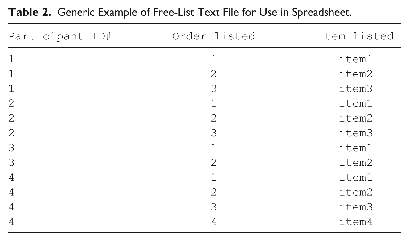
One might also organize free-list data in a spreadsheet with the format detailed in Table 2. This method is helpful for conducting cross-cultural work in teams, as it is intuitive for those who typically work in a spreadsheet format and spares researchers the effort of creating long text files. This method is also helpful for creating quick tables with spreadsheet software (e.g., “pivot” or “pilot” tables in Excel or Calc, respectively). However, subsequent calculations (e.g., of item salience) or transformations (e.g., dichotomizing presence and absence) can be time-consuming and prone to error, particularly if one has a large data set with many participants and groupings. If researchers are not inclined or able to write and maintain macros that often require updating with subsequent versions of software, these tasks can be especially tedious and frustrating if specific functions do not work or require debugging. In addition, macros for one office suite rarely transfer to others making the analyses difficult to achieve without the right software, and hindering transfer of relevant macros between researchers.
Generic Example of Free-List Text File for Use in Spreadsheet.
AnthroTools overcomes these limitations and allows researchers to (a) quickly analyze free-list data; (b) convert them into various data sets that are more immediately usable for merging with other data and subsequent analyses; (c) take advantage of the versatility of the free, open-source language R (R Core Team, 2012) that has a plethora of extant packages that handle typical analytical accompaniments to free-list tasks (e.g., multi-dimensional scaling, correlational matrices, principal components analysis, regression, etc.). R has full graphics capabilities and handles a variety of data file formats. AnthroTools also (d) includes built-in help files with illustrations and examples for ease in use. And, in the event that researchers already have data in the ANTHROPAC format (.txt files), it can readily convert data in this format into a standardized spreadsheet for immediate use.
As described in more detail below, we also created a variety of options for transforming free-list data into useful tables for further integration and analysis (e.g., using free-list data as a dependent or independent variable, running principal components analysis, etc.). These options include (a) tables with binary data indicating whether or not an individual listed a specific item (ideal for logistic regression), (b) tables of the frequency of items (ideal for free-list data that are subsequently coded using a standardized coding rubric), (c) tables that report the sum of salience for each individual item per participant, (d) a table including the order values of listed items, and (e) a table reporting the maximum salience for each item per individual. Subsequent generation of participant × participant or item × item matrices (e.g., for use with multi-dimensional scaling) are already built into R’s framework. Virtually every other step from this stage in analysis is already available in R’s many other packages and default functions.
Cross-Cultural Free-Listing
Researchers regularly use free-lists to rapidly make sense of cultural models within a sample. However, cross-cultural researchers may wish to collect data in the same or similar cultural domains from multiple sites or from multiple groups (e.g., Purzycki et al., 2016). Indeed, we developed the software to handle such cross-site data quickly and efficiently. For example, if your theory predicts that Item X will be more salient in Group Y than in Group Z, then grouping salience scores is necessary. If you predict that a certain class of items is going to be more prevalent in one group or another, again, grouping is imperative. If some domains should contain very similar items regardless of culture, once again, chunking salience and frequencies by group is required to effectively examine this. AnthroTools can chunk free-list data by any factor you wish (e.g., gender, religious group, cultural site, age group, etc.). Simply identifying how to chunk calculations will immediately generate cross-cultural sets, reports, and matrices that are ready for global and local analyses helpful for team-based cross-cultural research management. To illustrate, we offer a brief walkthrough of a free-list analysis below. Like many R packages, AnthroTools includes built-in examples for all of its primary functions. We highlight some of the main features in this article, but more functions and details are available within the package and in the package documentation on the website.
Walkthrough Example
To install AnthroTools, run the following code in R:
The only additional package upon which AnthroTools relies is “devtools” (Wickham & Chang, 2016).
Salience analysis
To illustrate, let us assume that you have data from people who freely listed the kinds of fruits they knew (Bernard & Ryan, 2009). After installing and loading the package, simply running
will call up the sample free-list data we created. To view the data set (Table 3), run:
Truncated Data Set of Freely Listed Fruits.
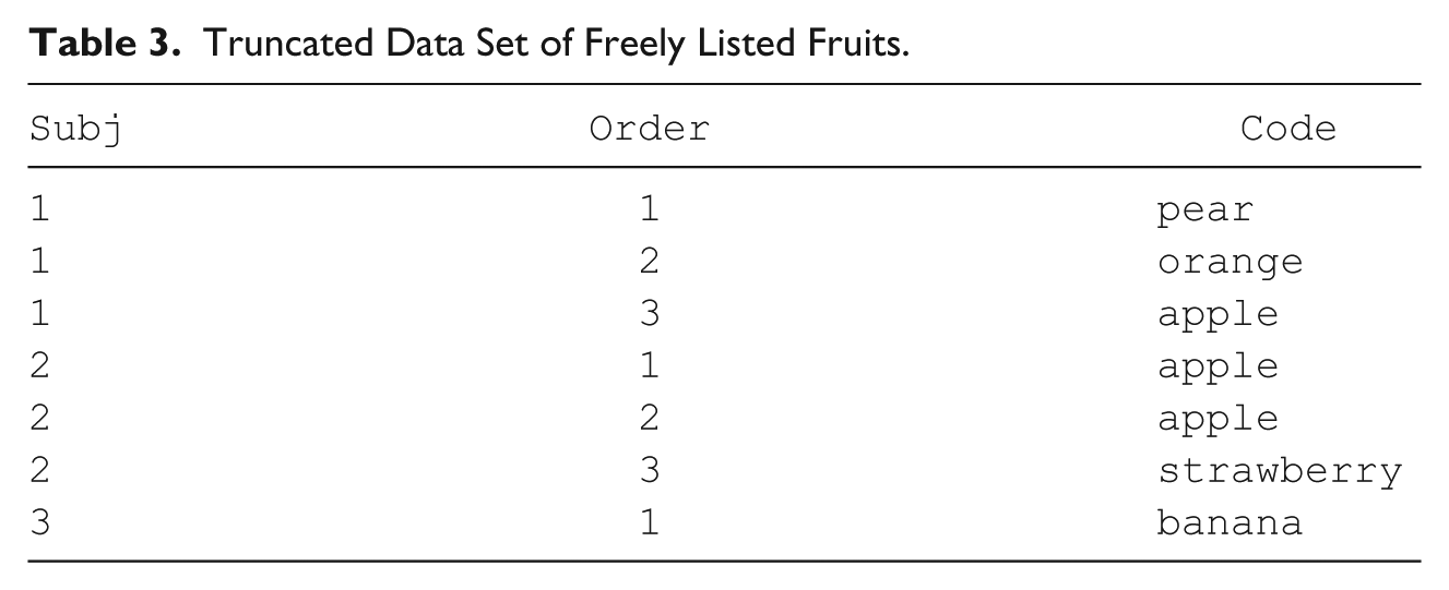
Note that in this data set, there are only three variables: “Subj” is the participant ID number, “Order” is the order in which participants listed items, and “CODE” is the data point. In total, there are 20 participants.
The CalculateSalience command generates each item’s salience score and creates a new column for this score. We will create a new object called “FL” that will be this new data set:
Table 4 is a truncated version of this new set with “Salience” scores added as a new column:
Truncated Data Set of Freely Listed Fruits After Calculating Salience.

The full syntax for CalculateSalience is as follows:
This allows you to call your variables whatever you want and associate them with the function’s operations (e.g., if your participant ID variable is called “ID” in your data set, the code would be Subj = “ID” for that component).
The function “SalienceByCode” takes this new data set with the by-item salience scores and creates another output specifically designed to handle overall salience by item code (Table 5). Run the following:
Salience Analysis of Free-List Items.
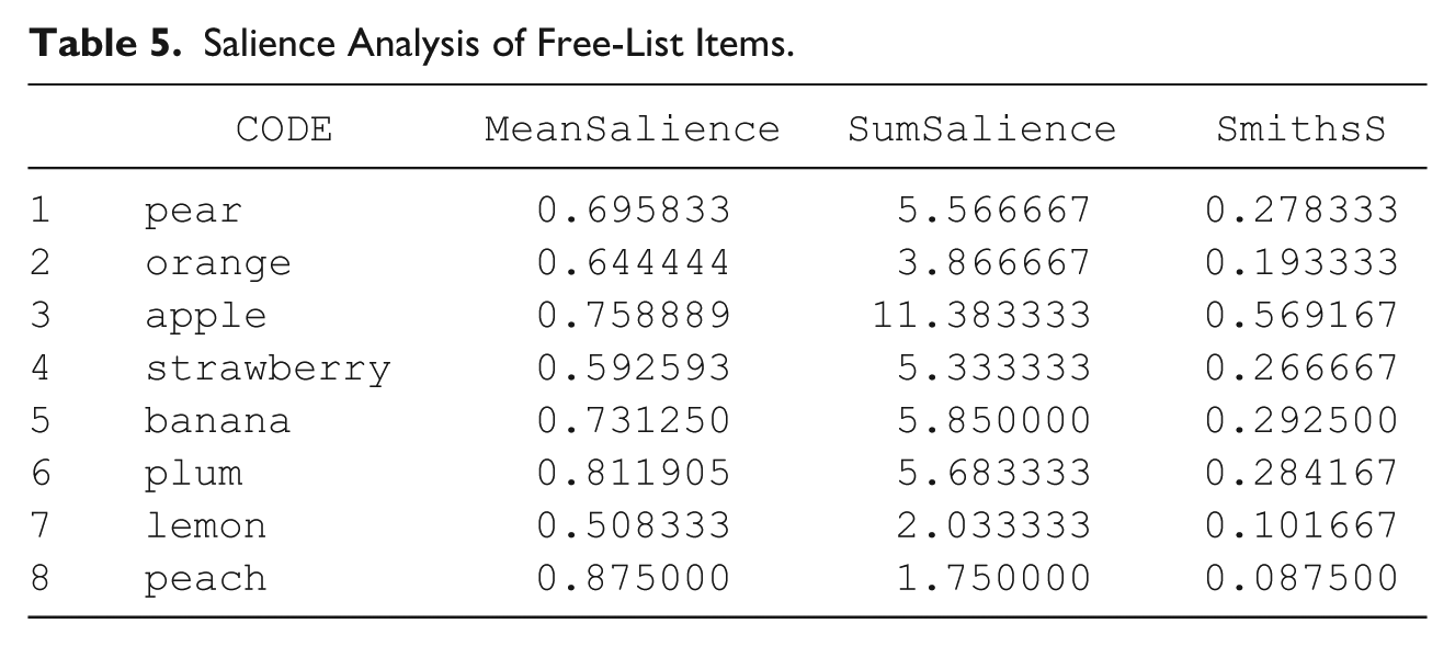
This argument calculates by-item mean salience and the sum of salience scores. It calculates Smith’s S by dividing the sum of salience scores by number of participants in the sample (again, in this case, n = 20; Borgatti, 1998; M. Quinlan, 2005; Smith, 1993; Smith et al., 1995).
As mentioned above, data points often get repeated due to individual responses or post hoc recoding. To avoid the subsequent inflation of Smith’s S values, we created the “dealWithDoubles” argument to allow flexibility in handling such instances. On the default setting, the function will assume that no such cases arise. If there are such cases, R will report an error and encourage you to use the “dealWithDoubles” command. So, if you run the same script above, but delete the “dealWithDoubles” argument, you will see the error notifying you of repeated items (notice that Subject 2 lists “apple” twice).
Aside from DEFAULT, you also have the options MAX, MEAN, SUM, and IGNORE. MAX indicates that you want the computer to attend only to the first time a respondent lists a particular CODE, and ignore subsequent mentions (e.g., if someone lists “apple” twice, it only keeps track of its earliest listing). For MEAN, the computer determines each respondent’s mean salience for repeated items and uses this value to calculate Smith’s S. For SUM, you are asking the computer to determine each respondent’s total salience with respect to a given code. If this value is greater than “1,” R will report an error identifying the source of the problem and recommend normalization (see below). IGNORE is merely a way of suppressing errors and is thus not recommended. The full syntax for SalienceByCode is as follows:
Tables for further analyses
As noted above, we created a variety of options for transforming free-list data into useful tables for further analyses (e.g., using free-list data as a dependent or independent variable, running factor analysis, etc.). The general syntax is as follows:
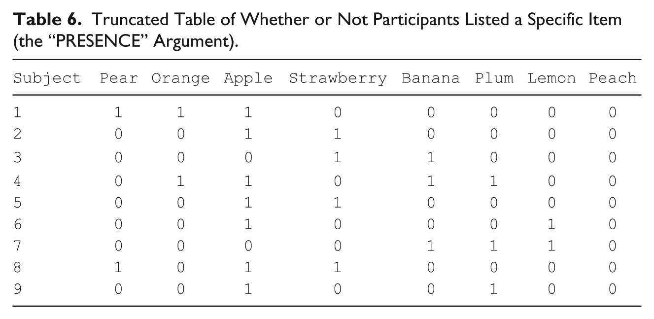
Currently, there are five types of tables: “PRESENCE,” “SUM_SALIENCE,” “MAX_SALIENCE,” “HIGHEST_RANK,” and “FREQUENCY.” “PRESENCE” converts data into a “1” if participants mentioned the specified code and “0” if they did not (Table 6). This might be helpful for logistic regressions where your dependent variable is whether or not someone listed a specific type of item or to generate proximity matrices. If you use “SUM_SALIENCE,” then you will get the total salience each person has associated with each code. If you use “MAX_SALIENCE,” then you will get the maximum salience, that is, the salience of the code the first time it was mentioned. “HIGHEST_RANK” creates a Participant × Item matrix of the order in which each item initially appeared for each individual. These are especially useful for multi-dimensional scaling to craft visual mental maps of items. If you specify “FREQUENCY,” then you will get a count of how often each code was mentioned by each person. This might be useful in general linear models, especially when your data consist of relatively frequently repeated items. Quick summations for each column can be made with R’s built-in colSums() command. To illustrate, if we run the following code on the FL data set, we get a table with binary presence/absence data for lists.
Truncated Table of Whether or Not Participants Listed a Specific Item (the “PRESENCE” Argument).
Again, such tables may be useful in and of themselves or in tandem with other data sets of the same participants to make predictions about or using frequency and salience. Moreover, cross-cultural variation in item salience is also of importance and interest. If, for instance, you conduct the same free-list task among multiple, culturally disparate groups, chunking salience by group may be necessary. We now illustrate this procedure in AnthroTools.
Grouping salience calculations
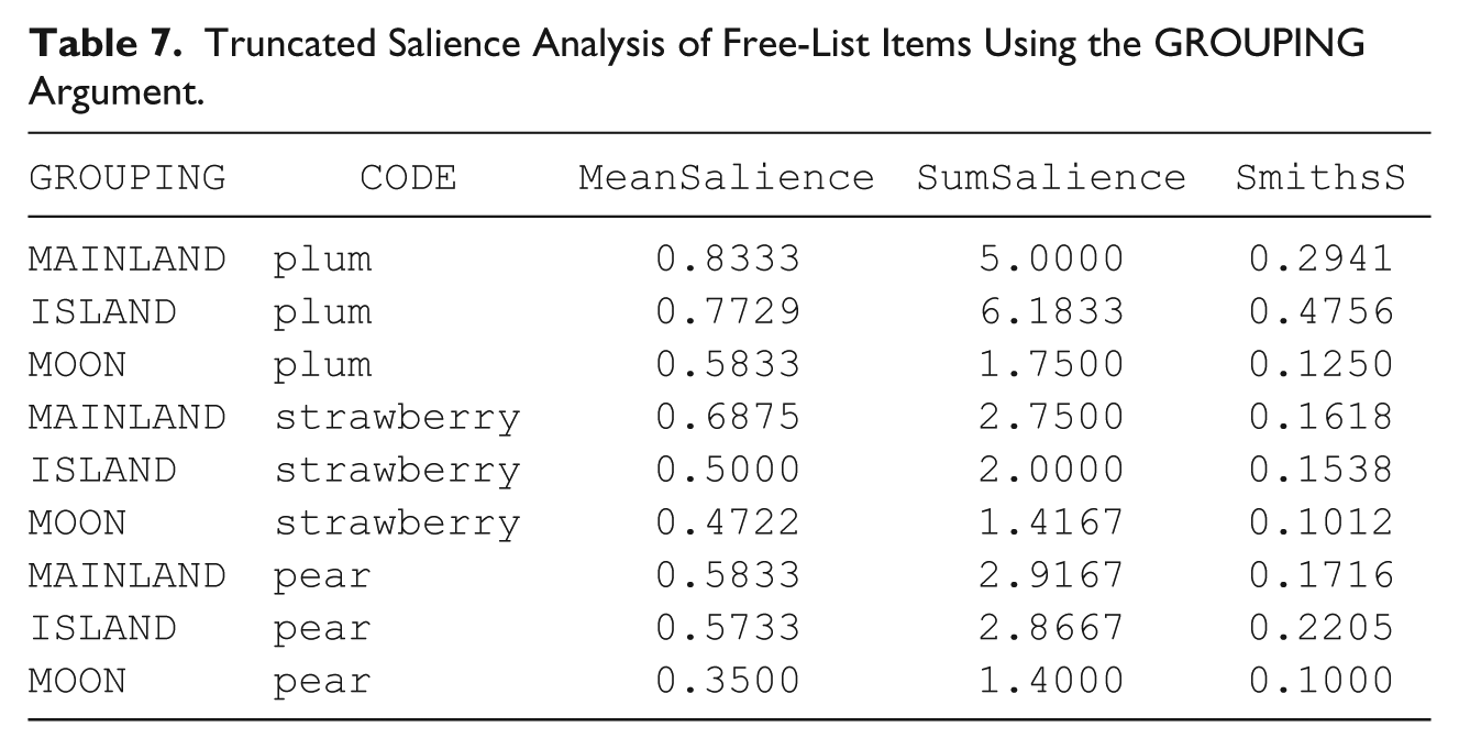
Grouping allows salience analysis to be carried out on individuals belonging to different groups (e.g., different field sites). This option is optimal for cross-cultural or any comparative study where participants are grouped by any given factor. Again, simply identifying which factor you wish to consider by using the GROUPING argument will perform the full task. Subject code overlap between groups is permitted, and salience calculations can be done on a group-by-group basis for each item code. The following includes syntax for the toy example included in the package. You will see that the final output is a table calculating salience by item, by group.
The output will look something like Table 7. The GROUPING variable here divides the analysis by sample or cultural group—the mainlanders, people from the island, and some people from the moon. Note that we sorted by CODE. Mean salience, sum of salience scores, and Smith’s S are all calculated based on within-group sample sizes (we truncated the table and the decimal places). The FreeListTable function also works with the grouping argument, so one may generate similar data sets (binary, frequency, etc.) with the grouping variables intact.
Truncated Salience Analysis of Free-List Items Using the GROUPING Argument.
Cleaning free-list data
Free-list data and their analyses face common problems, and we designed AnthroTools to be able to address them
The second addresses variation in how many items participants list. In open-ended free-lists, some individuals will list many items thus swamping salience scores. AnthroTools can rescale and normalize salience scores across individuals. The third cleaning function addresses salience inflation. And again, as is often the case, data points get repeated; participants sometimes list specific items more than once. Alternatively, if free-list data are subsequently recoded using a prefabricated scheme, data will often appear to repeat (e.g., someone says “cat” and “tiger” and you wish to lump these together in your “feline” category). Repeated items can inflate Smith’s S values in automated analyses. AnthroTools handles such items with multiple types of corrections including calculations based on earliest listed repeated items and the mean salience of such cases.
Cultural Consensus Analysis
Cultural consensus analyses (Anders & Batchelder, 2012, 2013; Anders, Oravecz, & Batchelder, 2014; Caulkins, 2004; Miller, Kaneko, Bartram, Marks, & Brewer, 2004; Oravecz, Anders, & Batchelder, 2013; Oravecz, Vandekerckhove, & Batchelder, 2014; Romney, Weller, & Batchelder, 1986) were designed to assess inter-informant agreement, expertise, and cultural knowledge. It is especially suitable for multiple-choice and dichotomous yes/no questions, where the interviewer does not necessarily know the correct answer or where the notion of a “correct” answer may itself be misguided. The traditional form of analysis searches for correlations between respondents’ answers and uses these to infer the level of “expertise” of each respondent, before going on to determine which answer is considered correct by the majority of respondents (weighted such that more attention is paid to respondents with greater expertise). By conducting consensus analysis with multiple groups, a researcher is able to systematically determine similarities and differences in what answers are deemed “correct.”
Such analysis might be applicable to such questions as “What is the name of this plant?” or “Out of these five examples, which is most likely poisonous?” or “Is your deity omniscient?” Indeed, consensus analysis has been useful in a variety of domains ranging from evaluations of which material items indicate being a successful individual (Dressler, 1996) and social views of the wives of miners from Yorkshire (Caulkins & Hyatt, 1999) to assessments of traffic medians and safety (Kim, Donnell, & Lee, 2008) and European views on obesity (Ulijaszek, 2007).
The analysis depends on several main assumptions (Hruschka & Maupin, 2013; Romney et al., 1986), but the two most crucial are that questions have a single “correct” answer and that all questions are in the same domain. The traditional form of consensus analysis rests on the assumption that you are asking multiple-choice questions, and that for any given question, participants know the answer to the question with some probability p and guess the answer with some probability 1 − p. Here, p is expected to vary between participants depending on their “competence” but does not vary between questions; it is assumed that all questions are of similar difficulty and within the same domain of knowledge (see more below).
Successful consensus analysis will produce two major outputs. First is an answer key for your survey items; it will tell you what the “correct” answer is for each question based on a variety of calculations. Second, it generates competence scores for each individual, indices that approximate the degree to which each participant resembles the cultural model.
The Logic of Cultural Consensus Analysis
This section explains the traditional logic behind cultural consensus theory and analysis, followed by sections reviewing extant software and a walkthrough example of consensus analysis in AnthroTools.
The first step in the analysis is to estimate the value of p—the probability of knowing the right answer—associated with each individual. This is done by finding the correlation between individuals’ answers,
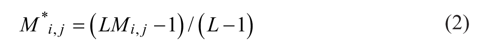
Here, L represents the number of possible answers to a given question.
Assuming all questions and individuals are relatively independent of one another, this value (the rate of both knowing the answer) should be equal to the product of the p values for the two individuals. 1 Thus, for every pair of individuals, we have the following equation:
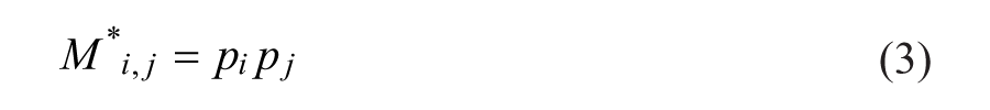
Here, we refer to the i,jth entry of the matrix, and the values of p refer to the competence of subjects i and j.
In general, this system will result in more equations than unknown variables, and thus cannot be solved exactly. However, assuming that all the assumptions of consensus analysis have been met, the set of equations should be approximately soluble. The AnthroTools package does this using what we will call the “Comrey Iteration” (Comrey, 1962, see more below). 2
Once we have determined the competence scores of each individual, the “correct” answer to each question can be inferred from the survey by using Bayes’ theorem:

In the particular case of consensus analysis, this translates to “the probability of answer A being correct for Question 1 given our current survey results is equal to the probability of seeing this particular series of answers given that A was correct, multiplied by the prior probability that A was correct, and divided by the probability of seeing this particular series of answers (without knowing anything about the answer).” 3
Walkthrough Example
Basic consensus analysis
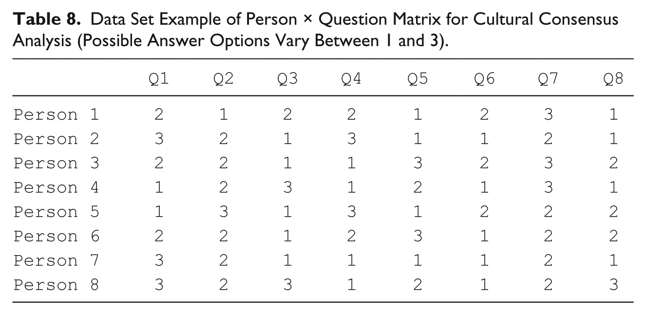
AnthroTools automates consensus analysis with the “ConsensusPipeline” function. The following is a walkthrough of our toy example. First, call up the data set:
Table 8 represents the example data set:
Data Set Example of Person × Question Matrix for Cultural Consensus Analysis (Possible Answer Options Vary Between 1 and 3).
To run the consensus analysis, simply invoke the function “ConsensusPipeline” and indicate the number of total possible answers to your multiple-choice key (in this case, it is 3):
These results contain the calculated answers, the competence assumed for each person, the actual test scores found for each person (assuming the answers calculated are correct), and the probability distribution for each of the answers. Note that in general, we are primarily interested in the answers calculated, but looking at the other results can be useful for informing you if your input has led to strange results (e.g., negative probabilities). Output 1 has the following elements: $Answers, $Competence, $origCompetence, $TestScore, $Probs, and $reportback.
Output 1. Cultural consensus analysis output
The $Answers section provides the culturally “correct” answers provided by the function, whereas $Competence reports the estimated cultural competence for each individual. In this case, then, Persons 2 (≈ 0.73) and 7 (≈ 0.97) had the highest two competence and test scores, suggesting cultural expertise. $origCompetence is the competence score before the transformation into the [0, 1] range. Assuming, of course, that the answer key is correct, $TestScore reports test scores for each individual whereas $Probs is the probability that each answer is correct for a given question. For example, 0.9984683724 is the calculated probability that “3” is the correct answer to the first question, while 0.955268538 is the program’s belief that “1” is the correct answer for question four.
We also provide various qualitative reports in the output. $reportback gives important feedback from the analyses. In the case of strange results, it may be worthwhile to examine whether or not the assumptions have been satisfied. The return value “reportback” has a written summary detailing such anomalies, including the competence scores that are out of bounds, along with the “Comrey Ratio” 4 used to determine whether it is likely that a single domain is present. “reportNumbers” yields the raw numbers from this summary, should you wish to analyze them.
In particular, for the above analysis, we notice that the “Comrey Ratio” is below 3. According to a standard “rule of thumb” ratio commonly referenced in the literature (e.g., Borgatti & Halgin, 2011; Weller, 2007), this ratio can be used to determine whether or not the assumption that all participants belong to a single unified culture (with a single correct answer key)—if this ratio is three or above, the assumption of a single unified culture is treated as valid; below this ratio, the assumption is considered suspect. However, in $reportback, the reported ratio was ≈1.32. This indicates that, according to this rule of thumb, the above survey cannot be assumed to come from individuals of a single culture, despite the fact that the data are computer-generated and were generated in a manner satisfying all assumptions of the model (single culture, independent answers, all questions in a single domain with equal difficulty).
Stress testing
To explore this phenomenon, we created the functions “GenerateConsensusData” and “ConsensusStressTest,” the former of which can be used to simulate a single survey, whereas the latter can simulate a large number of surveys and then perform consensus analysis on each of them. As input, they both take a number of individuals (per survey), a number of questions, and a number of allowable answers (per question). The Stress Test also requires the number of surveys to simulate. In both cases, the user can also choose to “lock” the competence of individuals setting all competence values of the group to the same value.
These functions prove useful when attempting to determine whether a given result is “normal” in some sense. Again, in our test case example above, we found the Comrey ratio to be only 1.32—well below the 3:1 ratio recommended rule of thumb.
The stress test reports back a wide variety of statistics (please see the command help(ConsensusStressTest) for full details), but in particular, it can be determined what fraction of surveys resulted in a ratio greater than 3:1:
Upon running the above command ourselves, we found that for this size of survey, a mere 1.2% of all simulated surveys were able to pass the 3:1 rule of thumb. This suggests that the threshold currently recommended in the literature may need to be reconsidered—possibly taking into account survey size and number of participants. Alternatively, other statistical tests no longer dependent on this ratio of factor weightings may be more appropriate. For now, however, in the absence of stronger systematic methods for assumption checking, we offer the Consensus Stress Test as a tool for generating “typical” data for the researcher to compare against statistically.
Current Software
Like AnthroTools, ANTHROPAC conducts consensus analysis, but not in its updated Bayesian formulation. Oravecz et al. (2014) created a standalone program that offers this alternative for binary data, and Anders (2014) created the R package CCTpack for those who prefer to remain within the framework of R and handle a variety of data using contemporary Bayesian estimations. Both have a variety of very sophisticated applications. Our observations so far are that these more thorough methods spend significant amounts of time in their parameter estimation, particularly for large data sets, whereas the more approximate method provided in our package provides a significantly quicker result. In cases where simply determining the “correct” answers is required, and your data set is large enough to limit the issues caused by approximation, AnthroTools may thus prove useful as a quick and streamlined exploratory measure (especially useful for field researchers), with the heavier tools offered by these sources used for validity testing and more advanced analytical techniques.
Conclusion
Our primary goals for developing this tool were to make free-list and consensus analyses easier to manage, readily accessible, more efficient, and immediately useable for field researchers interested in content domains. It should be especially helpful for researchers doing cross-cultural work, or working with large samples. It is our hope to inspire cultural anthropologists to use these powerful and useful methods who would otherwise avoid free-list data and cultural consensus analyses because of their backend work or mathematical esoterica. For those already using these tools, we hope this makes the process easier.
Footnotes
Acknowledgements
We thank Patricia Andreucci, H. Russ Bernard, Carol Ember, W. Penn Handwerker, Cristina Moya, John Shaver, Susan Weller, and Aiyana Willard for their input and also gratefully acknowledge our anonymous reviewers’ feedback. We dedicate this work to the memory of Roy G. D’Andrade.
Declaration of Conflicting Interests
The author(s) declared no potential conflicts of interest with respect to the research, authorship, and/or publication of this article.
Funding
The author(s) disclosed receipt of the following financial support for the research, authorship, and/or publication of this article: The Cultural Evolution of Religion Research Consortium (CERC), sponsored by the Social Sciences and Humanities Research Council of Canada (SSHRC), and the John Templeton Foundation financially supported the authors during the preparation of this work.