Consensus Analysis for Populations With Latent Subgroups: Applying Multicultural Consensus Theory and Model-Based Clustering With CCTpack

Abstract

Advanced consensus analyses are made available with the cultural consensus theory (CCT) framework, which is a model-based methodology used to closely derive the consensus knowledge of a group or population (e.g., a culture). The relevant data are their questionnaire responses about a subject domain. CCT has been established as a main methodology for ethnographic studies in social and cultural anthropology, and it has also been incorporated into other areas of the social and behavioral sciences as an effective information-pooling methodology. Recently, there are major advances in CCT, including (a) the multicultural extension, which can detect latent subgroups of a population, each with their own consensus answers to the questionnaire items; (b) the development of new models for several questionnaire designs, true/false, ordered category (Likert) scales, and continuous scales; (c) the estimation of important parameters that affect the response process; and (d) the development of Bayesian hierarchical inference for these CCT models. The joint analysis of these features positions such CCT approaches as some of the most advanced consensus analysis methods currently available. That is, they jointly (and hierarchically) estimate the consensus answers to the questionnaire items, the degree of knowledge (cultural competence) of each individual, the response biases of each individual, the difficulty (cultural salience) of each questionnaire item, and the subcultural group of the individual. In this article, we provide an overview of these major advancements in CCT, and we introduce CCTpack, which is currently the only software package available that handles all these extensions, especially (a) and (b).

Keywords

consensus analysis populations model-based clustering latent class models questionnaire data signal detection theory mixture modeling

Introduction

Consensus beliefs, opinions, and expertise are rich sources of information with many uses, ranging from applications to anthropology, social research, and politics; commercial, Internet, and service uses; evaluations of persons (e.g., expertise or belief detection) and items (quality); and more. Cultural consensus theory (CCT; Batchelder & Romney, 1986, 1988; Romney, Weller, & Batchelder, 1986; Weller, 2007), which involves information aggregation techniques and models, provides advanced methods to retrieve and calculate such consensus information. For example, Batchelder and Anders (2012) showed that CCT models can detect consensus answers better than the majority rule, even during cases of only six respondents; and Anders and Batchelder (2012) showed that CCT models are capable of detecting cultural subgroups with diverse beliefs, which would otherwise provide misleading conclusions about the dominant group consensus. Third, CCT models benefit from improved accuracy in consensus detection, as they filter out response biases and item difficulty in the aggregation—descriptive calculations, such as majority rule or response means, cannot obtain the same handling of variance (e.g., see Anders & Batchelder, 2012; Anders, Oravecz, & Batchelder, 2014; Batchelder & Anders, 2012; France & Batchelder, 2014; Oravecz, Anders, & Batchelder, 2013; Oravecz, Faust, & Batchelder, 2014; Oravecz, Vandekerckhove, & Batchelder, 2012). These kinds of developments can markedly improve the precision of our data analyses, consequently improving the kinds of inferences researchers can make about consensus, culture, and other valuable, latent information from collected data. Furthermore, Anders (2014) has recently developed an R package, CCTpack, that provides pipelined implementations and diagnostics for such CCT methods, and CCT model-based clustering (one or more groups) for binary, categorical, and continuous data. This article reviews these recent major developments, and demonstrates how CCTpack can be utilized by anthropologists to perform these advanced consensus analyses.

The following is an illustration: To learn about consensus beliefs about a particular topic (postpartum hemorrhage) and in a particular context (in Bangladesh culture), Hruschka, Kalim, Edmonds, and Sibley (2008) interviewed three groups with graded experience. These groups consisted of skilled birth attendants (S) who received formal training in birth attendance, traditional birth attendants (T) who are without formal training but employ traditional Bangladeshi techniques in birth attendance, and Lay-Women (L) who are without any occupational experience in birth attending. Example questions involved are as follows:

Is the mouth of the womb not closing after birth (atonic uterus) a cause of too little bleeding?

Is vitamin or blood deficiency treated with amulets or blessings?

Is a slow flow of bleeding a sign of normal bleeding?

A priori, one would expect that these different occupational groups would constitute several consensuses, and indeed Hruschka et al. (2008) found that the data did not satisfy the classic CCT guideline for a single consensus (e.g., the 3:1 eigenvalue ratio; Weller, 2007).¹ As a consequence of this violation, a CCT modeling before the developments of Anders and Batchelder (2012) would be invalid to apply. These authors hence introduced CCT models that can handle consensus data with subgroups, providing consensus analysis with model-based clustering. The culture number diagnostic was also updated, as to instead examine the number sizable eigenvalues before a linear trend is observed, which then relates to the number of consensus groups in the data. Then, the validity of the CCT model fit is tested as to how well it reproduces the eigenvalue trend in the data. Note here that these eigenvalues indicate the amount that the respondents agree with one another, and they are obtained from a factor analysis of the respondents correlated with one another. For this example data set, as displayed by the black line in the left plot of Figure 1, the eigenvalue trend provides for at least two sizable magnitudes before a linear trend is observed, suggesting multiple clusters of consensus.

Figure 1.

Principal component analyses of the respondent-by-respondent correlation matrix of the postpartum hemorrhage data, used to assess the number of underlying consensuses (groups) in the data.

In the study, three Bangladeshi groups were interviewed, but do they really form three subcultures of distinct beliefs? This question can be answered by applying multicultural CCT models specified at two and three cultures, and examining which performs better on the quality of fit diagnostics (discussed in more detail later). In this case, a two-culture model performed best on such diagnostics, and as displayed in Figure 1, each of the many model simulations (gray lines) clearly reproduces the eigenvalue trend of the observed data. With these developments, we thus obtain a model that can fit multicultural data and retrieve the consensus answers of each group—even when there are fewer consensus groups than the number of initial identities interviewed (e.g., S,T,L). Note that as an alternative approach to such multicultural modeling (model-based clustering), one may also consider running the three identities separately with single-culture CCT models. However, this assumes a priori that occupational experience will define each individual’s consensus group. Such an assumption could likely be false. For example, could there be some (T) traditional birth attendants who are also skilled in (or more practicing of) standard medical knowledge as the (S) skilled birth attendants? Could this also be the case for several (L) laywomen who have related occupations/interests? Could some (S) skilled birth attendants be more prescribing to cultural and spiritual beliefs? In these cases, the derived consensuses will be less accurate, and some individuals will not be correctly clustered or evaluated. In fact, we will see such results in the following output: Rather, occupational experience is correlated with but does not define consensus membership.

The CCT model fit results are illustrated in Figure 2, based on 14 respondents of each identity: S, T, L, and 50 questions.² The left plot provides the consensus expertise of each respondent (scale 0-1, ascending order) and their model-based clustering (“Cluster 1,” “Cluster 2”); the bottom row (S,T,L) is their original classification from the data. From here, it is clear to see that identity membership to cultural subgroups (S,T,L) does not guarantee that this individual’s belief/knowledge corresponds most closely to their identity membership. For example, the two clusters derived constitute the following: “Cluster 1,” a group largely in formal medicine (mostly S, some T, and two L), in which the T and L tend to have lower competency; and “Cluster 2,” a group largely in traditional practice (T, L, and two S) in which T and L tend to have similar competencies. Hence, some L and T in Cluster 1, for example, may have received education elsewhere about formal medicine regarding postpartum hemorrhage (and prescribe to this more than cultural practices), and the two S in Cluster 2 may persist with their cultural and/or spiritual beliefs (despite their professional practice). Note also that as previously mentioned, another advantage of such consensus modeling is the capacity to make person and item evaluations. Here, the professional expertise of some S individuals may be evaluated by their competency ordering in Cluster 1.

Figure 2.

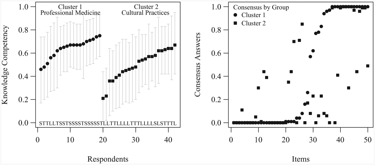
CCT model fit results on the postpartum hemorrhage data (42 respondents, 50 items).

Next, the right plot of Figure 2 provides the consensus answers (ascending order by Cluster 1) for each cultural subgroup for the 50 items (ordered likewise in Supplementary Appendix A, which also provides these answers). As discussed previously, prior work has shown that these model-derived answers can be more accurate than descriptive aggregations, such as the majority rule. Note that the values here, ranging between 0 and 1, represent the degree of consensus for these answers (or are probabilities of the answer being 1 or “true”).³ Indeed by observing the plot, a comparison of the two groups shows that similar consensus answers were obtained for about 30 of the items, and that the groups are actually distinguished by different beliefs for the other 20 items (where the squares do not overlap, or are distant from, the circles). Cluster 2 has more middling consensus values than Cluster 1. This result is rational, as formal medicine is less flexible in treatment protocol than in cultural traditions, which may be more susceptible to mixed or debatable protocols in treatment. Finally, we note that there are other useful parameters (e.g., item difficulty, response biases) that are estimated by the model, which improve the recovery of these consensus answers and groups, than CCT models (or other statistical methods) that do not include these parameters. These additional parameters shall be discussed in subsequent sections.

Through this introductory illustration, we have demonstrated the value and basic mechanics of model-based consensus analysis for multi- and single-cultural data. The readers who are interested to directly apply such methodology to their data may advance to the CCTpack walkthrough in Section “CCTpack Walkthrough” (note that the prior two sections “CCT Data Diagnostics” and “Interpreting CCT Parameters” are also helpful). The upcoming sections provide important information about CCT, its background, its variety of models, and generalities for how they are implemented. For example, the section “Development Over Time of Methods to Apply CCT and Relationships to CCTpack” discusses the developments over time in applying such CCT methods and other packages in relation to CCTpack. The section “The Hierarchical Bayesian Approach and Its Advantages for Consensus Analysis” discusses the hierarchical Bayesian estimation framework, which is used to implement such advanced applications. The section “The CCT Data Diagnostics for Binary, Ordered Categorical, and Continuous Consensus Data” more thoroughly explains quality of fit diagnostics, as provided in Figure 1, for assessing the validity of a model on a data set. The section “Interpreting CCT Model Parameters” provides an example demonstration of how to interpret the CCT model parameters after a model fit. Then, the section “CCTpack Walkthrough” provides a full walkthrough in CCTpack between data loading, model application, diagnostics, and results. The general discussion follows: Finally, Supplementary Appendix B provides a useful quick-reference guide for each of the CCT models that handle binary, ordered categorical, and continuous data (the models available in CCTpack).

CCT

In general, multiperson, questionnaire-based studies ultimately seek to discover an appropriate description of the underlying opinions, beliefs, or preferences of a given cultural population. Typical questionnaire data analyses usually involve aggregating the responses within each item using a central tendency measure, which can result in a crude summary of shared knowledge or preference. For example, these analyses can be improved upon considering that in many cases of real data, (a) populations may consist of a mixture of substantial subcultures, which are failed to be captured by central tendencies (and/or can perturb them); (b) human respondents vary in their knowledge expertise, and could be weighted accordingly in the aggregation; (c) questions may vary in perplexity or difficulty, and this could be accounted for as well; and (d), a more accurate aggregation also results when each individual’s response biases are filtered out of the total aggregation. These considerations have been developed into a formal, cognitive model-based data analysis methodology that advances above basic aggregation techniques, by taking into account these population (or subcultural) component clusters and influential cognitive factors. This described methodology comprises the essence of CCT, especially its recent developments.

CCT, also known as an advanced consensus analysis framework, is applicable to what we term as consensus data. Consensus data can hence be summarized by four characteristics: a set of individuals providing responses to a set of items that pertain to a shared knowledge domain, where each respondent may be appropriately clustered into a group that shares a consensus (e.g., a culture, or a group with individuals ranging in knowledge about a common set of “culturally” correct answers). In such questionnaire studies, both the number of latent consensus groups and the consensus answers of each group are usually unknown. Providing answers to, as well as the details about these unknown factors, describes the principal roles of CCT methodology, and especially why such multicultural diagnostics and detection methods can be valuable for such research projects. Particularly, the recent developments of CCT that we focus on involve model-based clustering methods to appropriately estimate these features, as well as cognitive metrics pertaining to the individuals/items themselves (e.g., respondent knowledge, response biases, and item difficulty). These cognitive factors may substantially affect the response process, and are hence used to improve the model fit accuracy of the cultures (clusters) retrieved and their latent consensuses. This is done by effectively weighting respondents according to knowledge, accounting for accuracy issues across items of varying difficulty, and filtering out individuals’ response biases from final aggregates.

Noteworthy Advancements in CCT

The beginnings of CCT methodology were developed in the 1980s (Batchelder & Romney, 1986, 1988, 1989; Romney, Batchelder, & Weller, 1987; Romney, Batchelder, & Weller, 1986). The methodology principally involved a canonical model (the General Condorcet Model [GCM]) for data consisting of a single culture (or a single-culture assumption), in which the individuals have made binary (true/false, yes/no) responses to a questionnaire about a shared knowledge domain. Inferences from this fundamental approach have been used extensively in anthropological research (see Weller, 2007). Recently, CCT modeling capabilities have been largely advanced in at least four ways: (a) to more data types than just binary data, such as to ordered categorical data (Anders & Batchelder, 2013) and continuous data types (Anders et al., 2014), which, respectively, introduced two new CCT models; (b) to the detection of latent subgroups (multiple cultures) and their respective consensus answers for each of these data types, providing a model-based clustering methodology for cultural analysis (Anders & Batchelder, 2012); (c) to improvements in aggregation (e.g., more reliably deriving the consensus values) by parsing along influential factors such as respondent biases, level of knowledge, and the item difficulty parameters that are estimated (e.g., Batchelder & Anders, 2012; Oravecz et al., 2013); and (d) to implementing the models with the hierarchical Bayesian framework (see aforementioned references), which, among various advantages, can improve parameter recovery in cases of smaller data sizes (Rouder, Lu, Speckman, Sun, & Jiang, 2005; Rouder, Lu, Sun, Speckman, Morey, & Naveh-Benjamin, 2007).

Development Over Time of Methods to Apply CCT and Relationships to CCTpack

We have emphasized some recent advancements in CCT methodology that notably consist of its extension to multicultural clustering models (and culture number diagnostics), as well as its extension to handle ordered categorical data and continuous data, in addition to the more classical binary data case. Importantly, hierarchical Bayesian implementations were also developed for all these model extensions, which facilitated the application of these more complex models. Hierarchical Bayesian implementations (see Kruschke, 2011; Lee, 2011; Rouder & Lu, 2005) can refine the quality of data aggregation (e.g., consensus and group derivation) by accounting for more factors that may substantially affect the response process.

Background

Prior to these advancements, the most popular CCT model was developed only for binary data, and it necessitated a single-culture assumption: The consequence is that the interpretations of the model’s parameters are only valid to the extent that one can prove the data consist of only a single culture. This model is usually termed the single-culture GCM (Batchelder & Romney, 1986, 1988; Romney et al., 1987; Romney et al., 1986). Since its beginnings, the single-culture GCM has served as a notably important and fundamental model for consensus analysis methodology, and has been extensively used in anthropological research (see Weller, 2007).⁴ To assess the single-culture assumption, CCT methodology has developed data diagnostics to help infer how many cultures may be existent in the data, such as by the eigenvalues obtained from a factor analysis (Comrey, 1962; Jolliffe, 2002) of the respondent-by-respondent correlation matrix (see Anders & Batchelder, 2012, for a detailed discussion).

Consequently, the first CCT packages were developed for the single-culture GCM, and are called ANTHROPAC (Borgatti, 1996) and UCINET (Borgatti, Everett, & Freeman, 2002). These packages allow application of the model with only heterogeneous knowledge competency, and otherwise fix response biases as neutral across respondents: For example, for all respondents, a 50/50 response guessing bias is used for items in which the respondent does not know the consensus answer. Hence, other factors that could improve data aggregation, such as heterogeneous response biases or item difficulties, cannot be estimated with these first packages. Both these packages utilized a clever but inferentially inefficient “method-of-moments” procedure to estimate the parameters of the GCM (see Batchelder & Romney, 1988).⁵ Then following these packages, Karabatsos and Batchelder (2003) developed the first software package to advance model estimation techniques for the single-culture GCM into the Bayesian framework (see Gelman, Carlin, Stern, & Rubin, 2014), as well as for the model to estimate heterogeneous response biases and item difficulties. By this development, they markedly advanced aggregation potential of the GCM; and they offer S-PLUS (Everitt, 2001) code with their article for this application.

Recent Bayesian Methods

Then, some notable advancements were recently made for applying the single-culture GCM to the Bayesian framework at further levels and customizations: First, Bayesian Cultural Consensus Toolbox (BCCT; Oravecz et al., 2012) offers nonhierarchical Bayesian applications of the single-culture GCM and estimation of all the response factors of the model (as well as the option to fix any of them as neutral). Second, the Hierarchical Condorcet Modeling Toolbox (HCMT)⁶ offers similar functionality (and some important extensions) but with the advance of hierarchical Bayesian model estimation. The usefulness of hierarchical Bayesian techniques in the context of CCT or cultural analyses is discussed next in Section “The Hierarchical Bayesian Approach and Its Advantages for Consensus Analysis.” The two notable and unique extensions provided in HCMT involve (a) a version of the GCM which allows individuals to respond with “Don’t Know” in addition to true/false, yes/no, A/B, and (b) the option to regress covariate (e.g., participant age, item length) effects on the estimated single-culture GCM parameters. For single-culture applications of the GCM, the HCMT is currently the most advanced package available, and offers the most customizability for this model. CCTpack is also a software package that provides hierarchical Bayesian implementations, and it will be discussed at the end of this section.

Recent Non-Bayesian Methods

Alternatively, there are several non-Bayesian packages for CCT applications that have been recently developed as well: First, there are CAML (Aßfalg & Erdfelder, 2012) and AnthroTools (Purzycki & Jamieson-Lane, 2017), which also fit simplified model versions of the GCM (restrictions to single culture) using maximum-likelihood methods as discussed in the first CCT packages; and furthermore, AnthroTools offers modeling methods for free-listing response data. Second, FlexCCT (France, Vaghefi, & Batchelder, 2013) is available, and can fit continuous responses to the single-culture case using maximum-likelihood methods, with two basic response bias options. One advantage of the maximum-likelihood approach is that it can generally achieve model fit in much less time than Bayesian inference, though at a cost of fitting more rudimentary model versions. Occasionally, these rudimentary models may be a poorer representation of the data when the influential factors comprising the data are more complex (e.g., multiple cultures, item difficulty, response biases).

CCTpack

Given these accounts, if one is interested in multicultural analysis with the GCM and/or single/multicultural analyses for ordered categorical or continuous data (notably with hierarchical Bayesian inference implementations), CCTpack is currently the only software package available that provides facilitated application of all of these models as well as their multicultural extensions. The package allows fitting all of the aforementioned cognitive parameters that can substantially affect the response process, such as heterogeneous knowledge competency, response biases, and item difficulty. The package can also handle participants who did not answer all the questions (missing data); and in the case of such missing data, the package provides estimates (makes predictions) of what a respondent would have answered to the items that he or she did not provide responses to. Furthermore, data diagnostics for the single/multiple cultural truth assumptions, based on mathematical properties of each model, are provided, which can help determine the number of cultures in the data. Furthermore, data diagnostics are provided to determine if heterogeneous item difficulty should be specified as well. In the following sections, we develop the approach by discussing the advantages of the hierarchical Bayesian framework, the CCT diagnostics for analyzing consensus data, and an overview of the three CCT models that, respectively, pertain to binary, ordered categorical, and continuous data that CCTpack provides. In Section “CCTpack Walkthrough,” a package tutorial (or walkthrough) is provided.

The Hierarchical Bayesian Approach and Its Advantages for Consensus Analysis

A noteworthy advantage of utilizing the hierarchical Bayesian framework as a model estimation approach for consensus research work is that it can minimize error in model estimation, and allow one to obtain more reliable parameter estimates in cases of smaller sample sizes (Rouder & Lu, 2005; Rouder et al., 2005; Rouder et al., 2007). This is typically achieved by modeling these samples of participants and items involved in the questionnaire study as sharing (statistical) properties from respective populations (e.g., items share properties more in common than the participants, and vice versa). Specifically, distinct stochastic population distributions, such as normal distributions, are specified as a source for the participants and items (and furthermore, subcultures can be modeled as from separate population distributions). In this way, the approach has been found to improve estimation for smaller sample sizes by constraining error and maximizing information that can be gained from the data (see Gelman, 2006; Kruschke, 2011; Lee, 2011; Rouder, Morey, & Pratte, 2015). For example, within-participant (or item) information is used to better estimate the between-participant (or item) information and vice versa (i.e., individual-level estimates are propagated to the group-level estimates and vice versa).

Furthermore, other reasons the Bayesian framework can improve reliability in estimation are that the parameters are estimated simultaneously; the parameters are integrated over the uncertainty of all other parameters, and as so, the error can be distributed more evenly across the estimated parameters. This is contrasted with maximum-likelihood or deviance minimization techniques, where estimations of one or multiple parameters can be serially done to derive the other parameters (e.g., from method of moment equations), in which error is more difficult to constrain or less evenly distributed. In addition, the Bayesian framework allows prior distributions to be specified for each of the parameters to further constrain error in estimation (see Gelman et al., 2014, for an explanation of Bayesian terms).

A second important note for why the hierarchical Bayesian framework is advantageous for consensus analysis, or these CCT model implementations, is that it is a framework which enables one to even apply such complex statistical models when it was not possible before to estimate such models. That is, the more complex expression of model likelihood that comes with these more advanced CCT models, for example, the multicultural extension and/or all of their cognitive metrics jointly estimated, renders them highly difficult to estimate with the more classical approaches, such as maximum-likelihood estimation. In fact, we currently do not know of any implementations of multicultural CCT models that are estimated with maximum-likelihood approaches. Thus, the Bayesian, especially hierarchical Bayesian, frameworks are quite valuable CCT model estimation approaches, and are capable of improving precision and performance in model estimation.

The CCT Data Diagnostics for Binary, Ordered Categorical, and Continuous Consensus Data

Validity of Group Measures

As noted previously, data aggregation measures (whether simple central tendencies or consensus model parameters) that describe a single population can be considered distorted or inappropriate measurements when the data involve subcultures / subgroups with notably different consensuses. Clustering these subgroups into their separate consensuses can improve the validity of the results. Alternatively, one might be interested to apply such a single-culture model to the data but provide a diagnostic based on mathematical properties, which supports the validity of a single-culture assumption. CCT methodology provides such kinds of diagnostics to discern appropriate assumptions of how many cultures are evident in the data and if the model satisfies them. We will discuss such diagnostics later in this section.

Quality of Data Aggregation

Second, we have noted that data aggregation can be improved by filtering the aggregation procedure according to factors that substantially affect the response process: For example, when individuals are weighted by their knowledge, and their response biases are filtered out, item difficulties can help us better estimate individual knowledge. For example, better estimates of individual knowledge may be obtained when we account that beginners may often get the easy questions correct, but often only the experts get the harder questions correct. When we estimate heterogeneous item difficulty, we can potentially improve model estimation. Furthermore, such improved data aggregation can improve the precision to which the consensus answers are recovered. However, sometimes this can make the model more difficult to estimate (e.g., longer model estimation time, clusters more intensive to recover), and CCT also has a diagnostic for if heterogeneous item difficulty is recommended for fitting the data.

These two aforementioned diagnostics have been developed for single/multicultural and hetero/homogeneous item difficulty, CCT models for binary data, ordered categorical data, and continuous data (which are overviewed in the next section); and CCTpack involves automatic generation of these diagnostics. Guidelines for how they are used and function are as follows (see also Anders & Batchelder, 2012, 2013; Anders et al., 2014, for more mathematical details):

Model Fit Diagnostic for Culture Numbers (Groups)

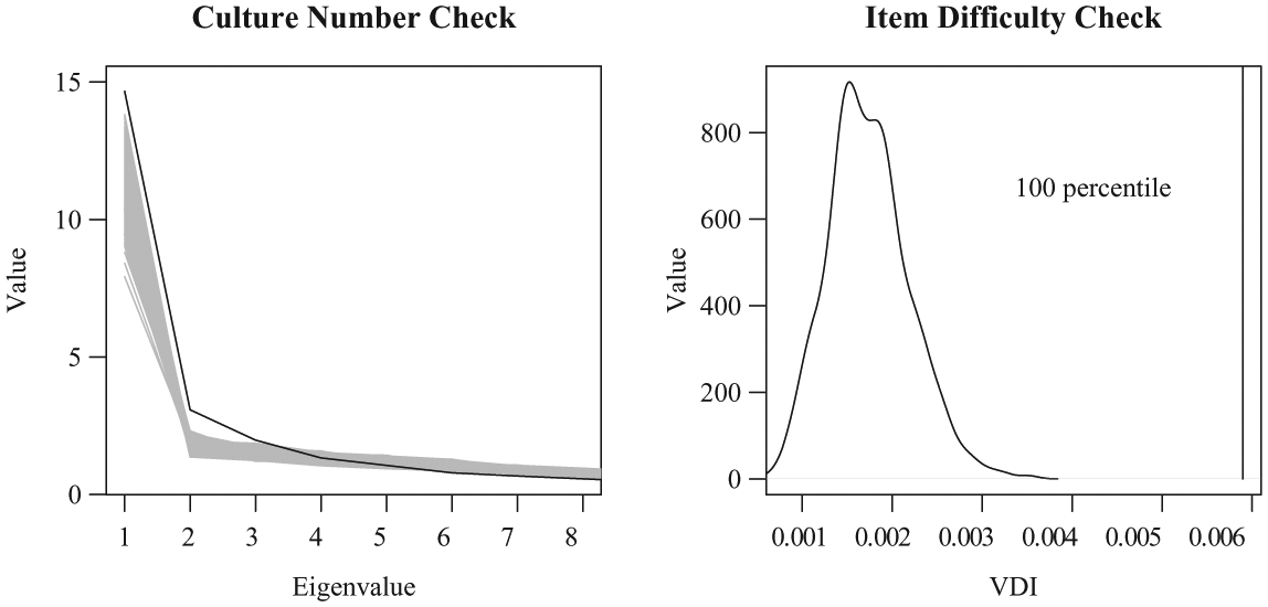
Based on mathematical properties of each of these models for binary/categorical/continuous data, the factor coefficients (e.g., eigenvalues) that pertain to how well the respondents agree with one another (e.g., of the respondent-by-respondent correlation matrix) may be obtained by a components analysis, and then plotted. This is commonly referred to as a scree plot; see the black line in the left plots of Figures 3 and 4. The number of sizable factors existent before an approximate linear trend is produced has shown to provide a reasonable indication for how many consensus groups may be existent in the data. Hence, before specifying how many cultures to fit a CCT model, it is recommended to inspect these scree plots, which we can produce from analyzing the respondent-by-respondent agreement trends in the data. Then, following a successful CCT model fit of the data, it is important to determine if the model has appropriately captured the scree plot trend that the original data produced. This is done by what is called a posterior predictive model check. In such a check, using the model parameters obtained from the model fit to the data, data sets are simulated (here 500 random sets), and hence checked if they correspond to the actual data observed. A scree plot is produced for each of these simulated data sets, and one observes if the simulated data sets appropriately correspond to the actual data set (Figure 3, left plot) or alternatively, fail to satisfy this diagnostic (Figure 4, left plot). Note that as the size of the first eigenvalue is often proportional to the total number of participants, in cases of large data sets (e.g., many participants) one may need to zoom in on the first several factors to better asses this diagnostic. This proportionality characteristic may also explain why the previous rule-of-thumb 3:1 eigenvalue ratio (e.g., see Weller, 2007) to assess the single-culture assumption may often fail to detect subcultures in large data sets (e.g., Hruschka et al., 2008).

Figure 3.

CCT culture number (left) and item difficulty (right) diagnostics.

Figure 4.

CCT culture number (left) and item difficulty (right) diagnostics.

Model Fit Diagnostic for Item Difficulty

A similar kind of posterior predictive model check can be used to determine if heterogeneous item difficulty is recommended in the model fit. Though assessing this property comes second in importance to the cultural number diagnostic check, as the interpretations from the parameters obtained from a CCT model can still be considered appropriate when data are fit with homogeneous item difficulty (though to involve a coarser aggregation) than with heterogeneous item difficulty that may sharpen results. This diagnostic hence serves as a tool to determine to what degree it may be important to specify heterogeneous item difficulty. Particularly, it involves a statistic called the variance dispersion index (VDI), which involves a comparison of the variance of responses within each of the items across the items (see Equation 15 of Anders & Batchelder, 2012). Hence, if the VDI is large, how items are responded to is highly varied across items, indicating support for heterogeneous item difficulty and vice versa. As before, one can simulate data sets from the model parameter estimates and see if model-predicted VDI statistics fall in the range of the observed statistic in the real data, as in Figure 3 (right plot), or alternatively, fail to satisfy this diagnostic as in Figure 4 (right plot). Consequently, if this check is not satisfied with homogeneous item difficulty, then heterogeneous item difficulty is recommended to be specified in the model.

Interpreting CCT Model Parameters

After a successful application of the model and verification of its fit diagnostics, an interpretation of the model parameters may be pursued. As previously mentioned, current CCT model applications can maximally provide (parameters for the following) a derivation of the item consensus values, respondent knowledge, response biases, and item difficulties; and if a multicultural application is performed, then also the group membership allocation for each respondent (and each subculture’s answer key and item difficulties). A Bayesian model application will result in a distribution of values for each parameter, and generally the mean is used as a reliable point estimate for each parameter’s true value called a posterior mean value. Then around this posterior mean value, interval bars (similar to confidence intervals) are determined by the distribution of values (e.g., 95% of the values; see Kruschke, 2011, for more details).

Figure 5 provides a demonstration (as they would be plotted by CCTpack) of the point estimates for each of the model parameters from a Bayesian application of a multiculture (here, two-culture) GCM to binary data (e.g., yes/no, true/false, A/B questions). In fact, we include the results from the postpartum hemorrhage data discussed in the Introduction: 42 respondents, 50 questions. In the top-left plot of the figure, the binary item truths, Z, for Culture 1 are represented by black circle symbols, whereas the binary item truths for Culture 2 are represented by white square symbols. Note here, however, that they are not in ascending order by Culture 1’s values as in the Introduction/Supplementary Appendix A. Then, the second plot, containing the item difficulty for each item λ, has the same kind of circle/square notation; 0 corresponds to the easiest items, 1 corresponds to most difficult. Here, the interval bars are not depicted to avoid excessive or obstructive markup within the plot. Note that for each parameter, the index v pertains to the culture number, and is hence in the set culture {1, 2}; and the index k is for the items and is in the set of items {1, 2, . . ., 50}. Then as for index i, these are the respondents in the set {1, 2, . . ., 42}.

Figure 5.

A demonstration of CCT model parameters obtained from a multicultural (two-culture) fit to binary data, using a Bayesian implementation.

Consensus Values

The consensus values Z, for each culture (v) and item (k), are provided as Z_vk in the first plot of Figure 5. As mentioned previously, here for the GCM, these answer values represent the degree of consensus. Hence, values close to 1 represent strong consensus of “yes/true/A” answers while values close to 0 represent strong consensus of “no/false/B answers.” Some previous CCT users may be accustomed to only dichotomous answers provided, without this more detailed information about the degree of consensus. These dichotomous answers are simply obtained by rounding these Z values (e.g., closest to 1 or 0). Then as for the other CCT models that handle item-scale questions, for example, ordered categorical and continuous data (Latent Truth Rater Model [LTRM]/Continuous Response Model [CRM]; see Figure 10), note that the consensus answers are instead called T_vk; they represent the item’s true position on the scale, and in this case, the degree of consensus is better discerned by the credible intervals (error bars).

Item Difficulty Values

The item difficulties, λ_vk, are provided in the top-right plot of Figure 5. They are also culture specific,⁷ and are ordered in the same correspondence as the consensus answers in the plot to the left. These λ_vk values reflect the difficulty to respond correctly to each question. For the GCM (the binary data model in the current plot), λ_vk = .5 is baseline level, so any values below .5 reflect the degree of item easiness, while values above .5 reflect the degree of item difficulty. Note that for the LTRM/CRM, λ_vk = .0 is the baseline level (see Figure 10), so likewise below 0 is easier while above 0 is harder. It is important to remark that these item difficulty parameter values provide for a better estimation of the consensus answers, as well as each individual’s knowledge or response dynamics. These parameters are described next.

Respondent Competency

The respondent competencies, θ_i, are provided in the bottom-left plot of Figure 5 for the 42 individual respondents. In this plot, the symbols represent the group memberships (model-based cluster assignments) of the individuals; respondents with a black circle belong to Culture 1, respondents with a white square belong to Culture 2. This symbology of the respondents corresponds to the same group symbology for the items in the top two plots of the figure. In the case of the GCM here, θ_i is the probability between 0 and 1 that the individual responds correctly to any given question, and λ_vk, the item difficulty, scales this in the case of a particular item. For the item-scale models (LTRM/CRM, example in Figure 10), this competency parameter θ_i is instead called E_i. It measures their deviation from detecting the item’s true position on the scale, and this parameter is also scaled by item difficulty, λ_vk.

Response Biases

The participant response biases, g_i, are provided in the bottom-right plot of Figure 5 for the 42 individual respondents. The symbology is the same as in the respondent competency plot (lower left) previously discussed. For the GCM, g_i is the probability between 0 and 1 that an individual guesses “true” (or the response coded “1”) on a question in which he or she does not know the answer. Then as for the item-scale models (LTRM/CRM, example in Figure 10), there are two response biases: a_i, that is, the extent to which respondents prefer extreme values (a_i > 0) versus middling values (a_i < 0); and b_i that is the extent to which respondents prefer values on the left of the scale (b_i < 0) or right of the scale (b_i > 0). Hence, baseline or neutral respondent biases for each of these parameters are given by a_i = 0 and b_i = 0.

Respondent Group Membership

The respondent group membership, Ω_i, does not have its own plot in Figure 5, but is instead depicted by common group symbols in the bottom two plots. Two clusters (cultures) were fit with this CCT model, so any person’s group membership is either 1 or 2. It is also worth noting that a respondent’s competency (bottom-left plot) is a reasonable indicator (though not decisive) for the matching strength of this person to his or her cultural cluster.⁸ Note that as we use a cognitive response model that parses for answer key, competency, item difficulty, and response biases, these latent clusters recovered by the model are advanced analyses compared to classic clustering approaches. In the following CCTpack walkthrough, we will show how to easily access these group membership values.

CCTpack Walkthrough

Being in the form of an R package, CCTpack is both widely accessible and freely available. The following subsections provide a demonstration of how to utilize the package, with a provided multicultural data example. The example data consist of a group of urban Guatemalan residents surveyed as to whether each disease (item) is better treated with a “hot” or “cold” remedy (Romney et al., 1986). The purpose of the investigation was to assess if ancient Mayan beliefs pertaining to whether certain diseases require a “hot” or “cold” remedy have persevered in urban Guatemalan culture. In this example data set, 14 random missing responses were added (of 23 respondents × 27 items = 621 total possible responses) to demonstrate the model’s capacity to handle missing data. Here, the data provide for a good practical example, especially due its smaller size (23 × 27), which allows for model fitting times on the scale of just a few minutes.

Installation

To get started, one must first download and install the general R software program from the official website:

https://www.r-project.org/

Then, JAGS (Plummer, 2003), which performs the MCMC sampling and tuning, needs to be downloaded and installed from the official website:

http://sourceforge.net/projects/mcmc-jags/files/

Once R and JAGS are installed, then the CCT package called CCTpack can be installed—it is currently hosted on the Comprehensive R Archive Network (CRAN). CCTpack can be downloaded and installed by typing the following in the R console:

install.packages(“CCTpack”, dependencies=TRUE)

The function setting dependencies=TRUE installs any R packages that CCTpack may depend on, and which your R version does not already have installed. Note that if compatibility issues are encountered, it is recommended that the user install the most recent versions of R and JAGS. Once CCTpack is installed, the package can be loaded within any R session using the following command:

library(“CCTpack”)

Loading Data

After loading the CCTpack library, the next step is to load the data that will be fit by the model. The example data of this walkthrough can be loaded using the command:

data(hotcold)

Then, these data can be accessed any time by typing hotcold.

Notes

Data for the package should be prepared in a matrix format in which the respondents occupy the rows and the items occupy the columns. Any missing responses to items should be specified as NA. When the data are appropriately specified, CCTpack will detect the number of respondents and items; the number of missing responses; the data type: binary, ordinal, or continuous; and selects the appropriate CCT model to analyze the data. Binary data will be analyzed with the GCM, ordered categorical data with the LTRM (Anders & Batchelder, 2013), and continuous data with the CRM (Anders et al., 2014)—see also the Appendix for a quick-reference guide of the models.

When loading data into CCTpack, keep in mind that at the time of this writing, CCTpack is currently developed to analyze the following three types of data formats: (a) binary data, coded 0 or 1; (b) ordered categorical data, coded 1, 2, . . ., C; and (c) continuous data, coded in (0,1). Therefore, the applicability of our data to CCTpack depends on whether it can correspond to one of these three data formats. Some data can be appropriately transformed to these formats. For example, continuous data with positive magnitudes can be appropriately transformed to (0,1) by using the following linear transformml: y = (x − min(X)) / (max(X) − min(X)), where X is the data matrix and x is the data cell value; and in the case of continuous data in the reals (e.g., −∞,∝), these values can be transformed to (0,1) with the inverse logit transformml: y = 1/(1 + exp(−x)). As a default, if continuous data are not transformed to (0,1) before they are loaded into the software, the inverse logit transform is automatically used by the program, in which the program will account for values of 0 as 0.001 and values of 1 as 0.999.

Specifying Cultures and Item Difficulty

Before fitting the model to the data, one should specify how many cultures (e.g., separate clusters that have distinct consensus beliefs) to estimate from the data. As discussed previously, the number of potential cultures in the data may be inferred from a factor or scree plot analysis (e.g., the number of sizable factors before a linear trend is observed). To produce the appropriate scree plot, the following command is used:

dat <- cctscree(hotcold)

The factor component values plotted in the scree plot can be accessed by

cctfac(dat)

For the Hot-Cold data, as illustrated in the scree plot in Figure 6, two substantially large apparent factors are exhibited. Thus, two cultures can be entered for the fit as clusters = 2. With regard to item difficulty, the questionnaire that gave rise to the data may have substantial differences across items (e.g., some diseases are more prevalent), so varied item difficulty is reasonable to estimate, and is selected as itemdiff = T. Note that different model fits may be assessed by the validation diagnostics (posterior predictive checks, for example, Section “The CCT Data Diagnostics for Binary, Ordered Categorical, and Continuous Consensus Data”), and subsequently by model quality of fit statistics, such as the Deviance Information Criterion (DIC; Spiegelhalter, Best, Carlin, & van der Linde, 2002), provided in this package.

Figure 6.

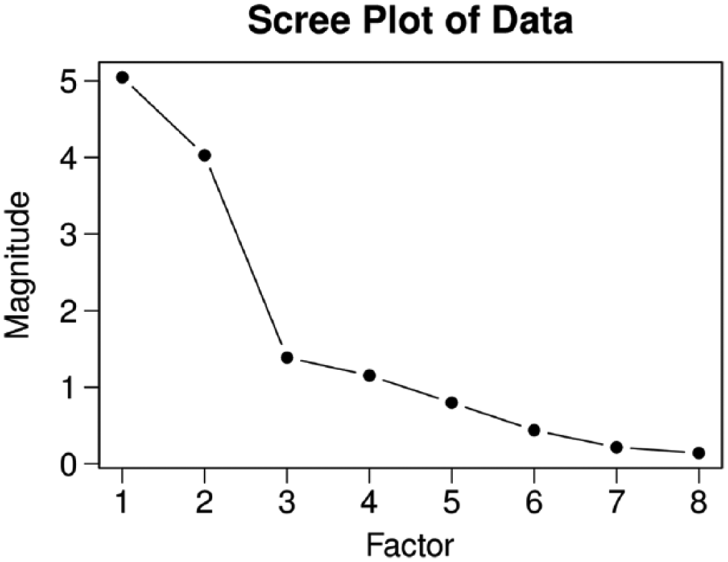
The scree plot generated from the dat <- cctscree (hotcold) command.

Applying the CCT Model

To apply the model with these settings to the data, the following command is used:

cctfit <- cctapply(data = hotcold, clusters = 2, itemdiff = T, seed = 1,samples = 10000, chains = 3, burnin = 2000)

The settings clusters = 2 and itemdiff = T, respectively, specify two cultures to be estimated, with heterogeneous item difficulty. Setting seed = 1 specifies the random generator, so if this command is run on another R session, the results should be replicated. The model will be estimated via hierarchical Bayesian inference. The fitting process takes an amount of time proportional to the complexity of the model, its assumptions (number of cultures, item difficulty), the size of the data, and the number of chains and samples specified. For example, due to their complexity, the LTRM or CRM may take noticeably longer to estimate than the GCM. When the inference is complete, the number of Rhats above 1.10 and 1.05 is reported, in addition to the DIC. Rhat, or $R$ , is a statistic that can indicate if a parameter estimate (through Bayesian sampling) may have nonconverged chains, and may be inappropriate to interpret (e.g., when $R > 1.10$ ). The DIC is a model fit criterion that may be used to compare the goodness of fit between two different model applications on the same data, in which lower values of the statistic are preferred (see Gelman et al., 2014, for a deeper explanation of Bayesian inference terms).

Notes

When a multiculture CCT model is applied to data, label-switching (Stephens, 2000) phenomena may occur. Label switching is defined by the situation in which the labels of the parameters between two or more MCMC chains are different, although they contain intended, corresponding data. For example, Culture 1 in Chain 1 may be labeled as Culture 2 in Chain 2; and the parameter values within these cultures will have highly similar, if not approximately the same cultural consensuses. When label switching occurs, the $R$ values will indicate that the chains did not converge, even though they may very well have. Label switching often occurs in fitting mixture models such as the multiculture CCT models, where the components are arbitrarily numbered during a MCMC run. To merge the data from several chains to estimate the posterior distribution of the parameters, it may be necessary to post edit the chains to bring the chains into conformity. The label-switching problem and its solution for multiculture CCT models are discussed in Anders and Batchelder (2012, 2013). CCTpack automatically applies such an algorithm to address this issue and returns the chains to the most consistent labeling possible. Thus after CCTpack applies its label-correcting algorithm, it will recalculate the $R$ values, so one may assess convergence accurately. It will also recalculate the DIC using the appropriate labeling.

Checking the Integrity of the Results

If the chains appear to have obtained proper convergence, then one may use the diagnostics discussed in Section “The CCT Data Diagnostics for Binary, Ordered Categorical, and Continuous Consensus Data” to assess the appropriateness of the model for the data. These two diagnostics, the culture number and item difficulty checks, can be calculated using the following command:

cctfit <- cctppc(cctfit)

One moment, calculating posterior predictive checks

Posterior predictive checks complete

[1] “VDI Culture 1 : 54.8 percentile”

[1] “VDI Culture 2 : 74.6 percentile”

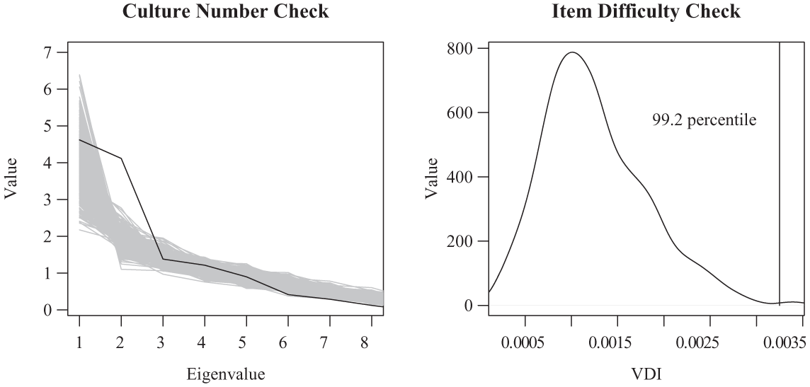
The command will produce the plots as in Figure 7, and give accompanying statistics (e.g., the VDI) for the item difficulty check. These checks can also be queued for calculation prior to the model run, by using the option, runchecks = T, in the cctapply() function. After the checks are run, their statistics, for both the model-predicted data and the observed data, can be, respectively, accessed by the following commands:

cctfit$ppeig cctfit$dateig

cctfit$ppVDI cctfit$datVDI

Figure 7.

The PPC plot containing the PPCs (diagnostics) that are important to verifying the validity of the number of cultures assumed and item difficulty options, and is generated from cctfit <- cctppc(cctfit).

The results in Figure 7 indicate that both checks are satisfied in this application. As discussed previously (Section “Interpreting CCT Model Parameters”), the culture number check is satisfied when the black line (scree plot of the data) is overlaying or highly similar to the gray lines (many scree plots produced from multiple data sets predicted by the model fit). Then, the item difficulty check is satisfied for the GCM when the VDI statistic for each culture lies within the 10th to 90th percentile of the distribution of VDI statistics, which is calculated from these many predicted data sets of the model fit.

Next, as in Section “The CCT Data Diagnostics for Binary, Ordered Categorical, and Continuous Consensus Data,” we demonstrate how these diagnostics can indicate if a model with poor specifications is applied to the data. For example, if one runs the single-culture model on the data set clusters = 2 and without item difficulty itemdiff = F, then Figure 8 shows that this model fails to satisfy each of these model checks. Particularly, the second factor is largely missed in the first plot, and the VDI of the real data is unsupported by being at the 99th percentile. Given that these two checks are instead satisfied with the first model, that is appropriately specified with two cultures and heterogeneous item difficulty, one can consider that the model’s psychometrics are appropriate for the respondents and items in the data. Thus when using CCTpack, when either of the two checks are found not to be satisfied, one may consider selecting a different number of cultures or a different item difficulty assumption for improved performance.

Figure 8.

Depiction of inadequate performance on the culture number check and item difficulty check; from running the model inappropriately specified at one culture and no item difficulty, on the example data set.

Viewing and Examining the Results

The posterior results of the model may be visualized by

cctresults(cctfit)

In addition, a tabular readout of the item answers, difficulties, and Bayesian-credible intervals is provided by the following commands:

cctitem(cctfit)

cctitemhdi(cctfit)

For example, using cctitem(cctfit), the following output is shown below: item is the item number; ans1_Z and ans2_Z are the consensus answers (in degrees of consensus), respectively, for Clusters 1 and 2; and Z is the parameter name (see top-left plot in Figure 9). These values can be converted to dichotomous answers simply by the command round(cctitem(cctfit)[,1:3]). Then, diff1_lam and diff2_lam are the item difficulty values, and “lam” represents the parameter name λ (top-right plot in Figure 9).

item ans1_Z ans2_Z diff1_lam diff2_lam

1 0.96 1.00 0.47 0.39

2 1.00 0.97 0.20 0.58

3 0.58 1.00 0.73 0.44

Figure 9.

The results plot containing posterior mean parameter estimates generated from the cctresults(cctfit) command.

Then using cctitemhdi(cctfit), the following output is given: While item is still the item number, there are eight columns here instead of the previous four for the item parameters. This is because these columns give the lower (l_) and upper (u_) Bayesian-credible intervals for each of these four parameters (ans1, ans2, diff1, diff2). These intervals are useful for interpreting the results or making your own plots of results. For example, the intervals used in the bottom plots of Figure 9 are obtained by cctsubjhdi(cctfit), which gives the subject parameter intervals:

item l_ans1 u_ans1 l_ans2 u_ans2 l_diff1 u_diff1 l_diff2 u_diff2

1 1 1 1 1 0.05 0.92 0.05 0.69

2 1 1 1 1 0.00 0.53 0.28 0.94

3 0 1 1 1 0.39 1.00 0.10 0.76

Then similar tabular readouts, but of the participant group memberships, competencies, biases, and Bayesian-credible intervals, are provided by the respective commands:

cctsubj(cctfit)

cctsubjhdi(cctfit)

The plot that is generated from the cctresults(cctfit) command is provided in Figure 9, which contains the model-estimated parameters for the N = 23 participants and M = 27 items. Note that if more than one culture is run, then the measures and memberships pertaining to each of the different cultures will be indicated by different symbols. For example, as in this case two cultures were specified to be estimated, in the first plot of the figure, the binary item truths for Culture 1 are represented by black circle symbols, while the binary item truths for Culture 2 are represented by white square symbols. Then, the second plot, containing the item difficulty for each item, has the same kind of notation. For each parameter, the index v pertains to the culture number, and is hence in the set culture {1, 2}; and the index k is denoted for the items and is in the set of items {1, 2, . . ., 27}.

In Figure 9, circles denote the first culture, whereas squares denote the second culture. The interval bars depict the 95% highest density intervals (HDIs; Kruschke, 2011); sometimes, interval bars are not depicted on the items (as in the top two plots) to avoid excessive or obstructive markup within the plot, but these intervals and further information may be gathered from accessing the cctfit data object, as in cctitemhdi(cctfit) or cctsubjhdi(cctfit). The bottom two plots of Figure 9 contain the cognitive parameters for the 23 individual respondents: knowledge competency and response biases. In these plots, the symbols represent the group memberships (model-based cluster assignments) of the individuals; respondents with a black circle belong to Culture 1, respondents with a white square belong to Culture 2. These cluster assignments may be viewed numerically with the cctsubj(cctfit) command.

In any readouts of the respondents and/or items (e.g., cctsubj(cctfit), cctitem(cctfit), equivalent to cctfit$subj and cctfit$item), the respondents and items are ordered in the same way as in the original data matrix that was loaded into the program. In a two-culture model, a value of “1” indicates that the respondent is estimated as a member of Culture “1” (the black circles in Figure 23, see the bottom two plots), and hence a value “2” indicates that the respondent is estimated as a member of Culture “2” (the white squares in Figure 23). Finally, note that interpreting the parameter values for each model may be difficult without a basic knowledge of the model. In this case, refer to Supplementary Appendix B and/or the original publications of these models: for example, for binary data, see Anders and Batchelder (2012); for ordinal data, see Anders and Batchelder (2013); and for continuous data, see Anders et al. (2014).

Quick Summary

A general summary of the fit object and data analyzed is provided by summary(cctfit), which produces the following output:

summary(cctfit)

Data: Binary Model: GCM

Respondents: 23 Items: 27

Observations: 98% Missing Values: 2%

Cultures: 2 Item Difficulty [X]

DIC: 740.54 pD: 133.82

Rhats > 1.10: 0 / 117 Rhats > 1.05: 0 / 117

PPC Calculated [X] VDI 55, 75

Samples: 12000 Chains: 3

Burn-in: 2000 Thinning: 1

As seen above, these statistics describe the data, the settings used for the fit, the quality of the fit, and the posterior predictive checks. As previously mentioned, we added 14 missing values to demonstrate the approach’s capacity to fit incomplete data. If cctfit <- cctppc(cctfit) has been run (e.g., as indicated by PPC Calculated [X]), then a table readout of these missing data estimates may be accessed by

cctmvest(cctfit)

Helpful Commands

summary(cctfit), cctresults(cctfit), cctitem(cctfit), cctsubj(cctfit), cctitemhdi(cctfit), cctsubjhdi(cctfit): Provide readouts and summaries of the model/parameter results, and their credible intervals (HDIs).

cctmvest(cctfit): If the data matrix has missing values, then after one has run the posterior predictive checks as cctfit <- cctppc(cctfit), the model will provide estimates of the most likely value for each respondent’s missing answers.

cctfit$ppeig, cctfit$dateig, cctfit$ppVDI, cctfit$datVDI: These commands, respectively, give the diagnostic statistics for model-predicted data and observed data (respondent agreement factor components and VDI statistics).

cctexport(cctfit,filename=“CCTpackdata.Rdata”): Will result in an R data object being saved with all of the information calculated; .JPEGs and .EPS files of the scree plot, results plot, and checks plot; and a .CSV file of the parameter estimates summary for quick reference. A quick save may be obtained by save.image(“CCTpackdata.Rdata”).

load(“CCTpackdata.Rdata”): Will respectively load the model fit results.

memory.limit(10000): Occasionally, multiple model fits may attempt to use more working memory than your computer has allocated for in R (for Windows OS). This will result in an R output error with an inability to allocate sufficient space. Frequently, this error can be resolved by augmenting the memory allocation to R. One can adjust this number to higher values for needed memory augmentations.

Example Results of the LTRM and CRM

CCTpack can also fit categorical and continuous data using the LTRM and CRM, and more details about these models are included in the Appendix. Note that as both the data type (more degrees of freedom) and the CCT models are more complex and advanced for these applications, the model run times are notably longer for these approaches.

Figure 10 contains example output of the LTRM model for ordered categorical data that has the simplified case of being single cultured (V = 1, hence all Ω_i = 1). This output may be produced using the following command:

Figure 10.

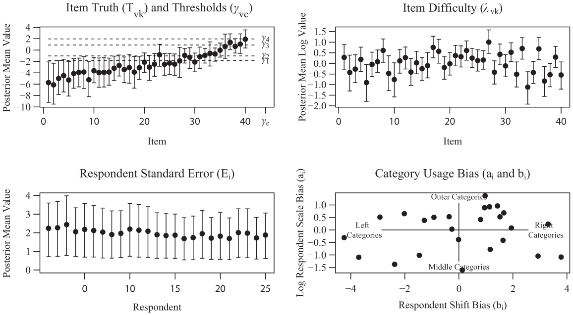
The results plot output from the model for ordinal (ordered categorical) data, containing posterior mean parameter estimates generated from cctresults(cctfit2).

data(raterdata)

cctfit2<-cctapply(data=raterdata, clusters=1, itemdiff=T, runchecks=F, seed=1, polych=F)

As before, table readouts of the parameter results can be obtained by cctitem(cctfit2), cctsubj(cctfit2), and the category boundaries γ_c in Figure 10 are obtained by cctcat(cctfit2). For categorical data using the LTRM, continuous truth values for the items, T_k, are estimated on the real line, as are a shared set of boundaries, the γ_c, among respondents, which describe the shared group responding tendency (category bins); both of these may be transformed back into the unit interval with the inverse logit transform to ease interpretation (as exp(x) / (1 + exp(x)). In addition, knowledge competency, E_i, and item difficulty, λ_k, on the positive reals are estimated, as well as response biases, a_i and b_i, which are plotted against each other to indicate individual responding tendencies that differ from the norm. One will also note that there is a polychoric correlation option for the LTRM polych = 1 in both cctapply() and cctppc(). Note that the polychoric correlations have been found to be more accurate for the categorical data scree plots and posterior predictive checks; however, they are much more time intensive to compute.

The CRM, the model for continuous data, estimates these same parameters as in the LTRM, except for the shared set of thresholds, as the continuous data are assumed not to be filtered through a set of thresholds to arrive at discrete increasing values (e.g., as opposed to the ordered categorical data). An example fit of the CRM may be achieved using

data(continuousdata)

cctfit3 <- cctapply(data = continuousdata, clusters=2, itemdiff=T, runchecks=0, samples=12000, burnin=2000, seed=1)

Discussion

A number of recent developments in CCT methodology and modeling have notably advanced its applicability and depth of data analysis, particularly (a) the capacity to detect latent subgroups in populations, each with their respective answer keys through model-based clustering and multicultural diagnostics, and (b) the ability to fit ordered categorical and continuous data in addition to the fundamental binary data case. Furthermore, improvements in accounting for factors that can substantially affect the response process (e.g., response biases, respondent expertise, item difficulty, cluster membership), as well as hierarchical Bayesian implementations for these models, have been made. These kinds of developments discussed herein can notably improve the precision of our data analyses, consequently improving the kinds of inferences researchers can make about consensus, culture, and other valuable, latent information from collected data. However, access to such methodology is difficult for nonexperts and those less acquainted with the approach. This literature has provided a concise, didactic overview of the methodology and its recent developments, and how CCTpack may be used to analyze data with these more advanced techniques. CCTpack discussed herein is currently the only software program developed to handle binary, ordered categorical, and continuous data for both single and multiple cultures (model-based clustering); and models the maximum number of factors currently developed in CCT to affect the response process (e.g., response biases, expertise, difficulty, cluster membership). This should improve the precision to which we infer the consensus answers, as opposed to simpler models. We have also discussed alternative programs readers may be interested in for other aims.

Future developments to CCTpack may consider greater customizability of the modeling specifications beyond those mentioned in this article and greater customizability of the Bayesian settings (though standard diffuse prior settings are specified already). Future developments may also integrate additional models that may be formulated in proceeding publications. Third, developments may also seek to reduce the model estimation time, particularly for the categorical and continuous data models, which tend to be notably longer to fit to the data. Nonetheless, currently CCTpack greatly facilitates access to CCT methodology to a wide readership, for which these techniques might otherwise be inaccessible, or at least much more laboriously accessible, such as by only a manual coding of the CCT models, their estimation techniques, the data and model fit diagnostics, and the model parameter plotting/interpretation.

Footnotes

Declaration of Conflicting Interests

The author(s) declared no potential conflicts of interest with respect to the research, authorship, and/or publication of this article.

Funding

The author(s) disclosed receipt of the following financial support for the research, authorship, and/or publication of this article: We acknowledge funding from the Centre National de la Recherche Scientifique (CNRS, French NSF); the following grants from the Agence Nationale de la Recherche :BLAN-1912-01, ANR-16-CONV-0002 (ILCB), ANR-11-LABX-0036 (BLRI), and ANR-11-IDEX-0001-02 (A*MIDEX); and a grant from the National Science Foundation (Grant #1534471) to the third author.

Supplemental Material

Supplementary material is available for this article online.

Notes

Author Biographies

Royce Anders is a postdoctoral researcher at Aix-Marseille University, France, specialized in human performance modeling, quantifying cognitive processes in decision making, developing cutting-edge measurement methods, and Bayesian approaches. He obtained his PhD in cognitive sciences from the University of California, Irvine, where he closely collaborated with the founders of classical cultural consensus theory. He was centrally implicated in launching a new wave of modern and advanced developments for the theory.

F.-Xavier Alario is a research director at the Centre National de la Recherche Scientifique (CNRS) in Marseille, France, specialized in cognitive psychology and language, with a number of involvements in methodological inquiry. His research examines psycholinguistics, human performance analysis, and experimental methods. More recently, he expanded his research toward the relationship between neurophysiology and cognition.

William H. Batchelder is professor of cognitive sciences at the University of California, Irvine, United States. He is highly regarded for his contributions in mathematical modeling and measurement methods in the social and behavioral sciences. Being one of the main founders of classical Cultural Consensus Theory (1986) and also being involved in major recent developments of the approach, his research is highly cited by anthropologists, psychologists, and social scientists.

References

Aßfalg

Erdfelder

(2012). CAML—Maximum likelihood consensus analysis. Behavior Research Methods, 44, 189-201.

Anders

(2014). CCTpack: Consensus analysis, model-based clustering, and cultural consensus theory applications to data (R package version 1.5.1). The Comprehensive R Archive Network (CRAN Repository), Retrieved from https://cran.r-project.org/web/packages/CCTpack/index.html

Anders

Batchelder

W. H.

(2012). Cultural consensus theory for multiple consensus truths. Journal for Mathematical Psychology, 56, 452-469.

Anders

Batchelder

W. H.

(2013). Cultural consensus theory for the ordinal data case. Psychometrika, 80, 151-181.

Anders

Oravecz

Batchelder

(2014). Cultural consensus theory for continuous responses: A latent appraisal model for information pooling. Journal of Mathematical Psychology, 61, 1-13.

Batchelder

W. H.

Anders

(2012). Cultural consensus theory: Comparing different concepts of cultural truth. Journal of Mathematical Psychology, 56, 316-332.

Batchelder

W. H.

Riefer

D. M.

(1999). Theoretical and empirical review of multinomial process tree modeling. Psychonomic Bulletin & Review, 6, 57-86.

Batchelder

W. H.

Romney

A. K.

(1986). The statistical analysis of a general Condorcet Model for dichotomous choice situations. In Grofman

Owen

(Eds.), Information pooling and group decision making: Proceedings of the second university of California Irvine conference on political economy (pp. 103-112). Greenwich, CT: JAI Press.

Batchelder

W. H.

Romney

A. K.

(1988). Test theory without an answer key. Psychometrika, 53, 71-92.

10.

Batchelder

W. H.

Romney

A. K.

(1989). New results in test theory without an answer key. In Roskam

E. E.

(Ed.), Mathematical psychology in progress (pp. 229-248). Heidelberg, Germany: Springer-Verlag.

11.

Borgatti

S. P.

(1996). ANTHROPAC 4.0. Columbia: University of South Carolina Press.

12.

Borgatti

S. P.

Everett

M. G.

Freeman

L. C.

(2002). UCINET for Windows: Software for social network analysis. Harvard, MA: Analytic Technologies.

13.

Comrey

A. L.

(1962). The minimum residual method of factor analysis. Psychological Reports, 11, 15-18.

14.

Everitt

B. S.

(2001). A handbook of statistical analyses using S-PLUS. London, England: Chapman & Hall.

15.

France

S. L.

Batchelder

W. H.

(2014). Maximum likelihood item easiness models for test theory without an answer key. Educational and Psychological Measurement, 75, 57-77.

16.

France

S. L.

Vaghefi

Batchelder

(2013). FlexCCT: Software for maximum likelihood Cultural Consensus Theory. Paper presented at the Conference on Educational Data Mining.

17.

Gelman

(2006). Prior distributions for variance parameters in hierarchical models. Bayesian Analysis, 1, 515-533.

18.

Gelman

Carlin

J. B.

Stern

H. S.

Rubin

D. B.

(2014). Bayesian data analysis (Vol. 2). Boca Raton, FL: Chapman & Hall.

19.

Green

D. M.

Swets

J. A.

(1966). Signal detection theory and psychophysics. New York, NY: John Wiley.

20.

Hruschka

D. J.

Kalim

Edmonds

Sibley

(2008). When there is more than one answer key: Cultural theories of postpartum hemorrhage in MATLAB, Bangladesh. Field Methods, 20, 315-337.

21.

Jolliffe

(2002). Principal component analysis. New York, NY: Springer.

22.

Karabatsos

Batchelder

W. H.

(2003). Markov chain estimation methods for test theory without an answer key. Psychometrika, 68, 373-389.

23.

Kruschke

J. K.

(2011). Doing Bayesian data analysis: A tutorial with R and BUGS. New York, NY: Academic Press.

24.

Lee

M. D.

(2011). How cognitive modeling can benefit from hierarchical Bayesian models. Journal of Mathematical Psychology, 55, 1-7.

25.

Macmillan

N. A.

Creelman

C. D.

(2005). Detection theory: A users guide (2nd ed.). Mahwah, NJ: Lawrence Erlbaum.

26.

Oravecz

Anders

Batchelder

W. H.

(2013). Hierarchical Bayesian modeling for test theory without an answer key. Psychometrika, 80, 341-364.

27.

Oravecz

Faust

Batchelder

W. H.

(2014). An extended cultural consensus theory model to account for cognitive processes in decision making in social surveys. Sociological Methodology, 44, 185-228.

28.

Oravecz

Vandekerckhove

Batchelder

W. H.

(2012). Bayesian cultural consensus theory. Field Methods, 26, 207-222.

29.

Plummer

(2003). JAGS: A program for analysis of Bayesian graphical models using Gibbs sampling. In Proceedings of the 3rd International Workshop on Distributed Statistical Computing (Vol. 124, p. 125).

30.

Purzycki

B. G.

Jamieson-Lane

. (2017). AnthroTools: An R package for cross-cultural ethnographic data analysis. Cross-Cultural Research, 51(1), 51-74.

31.

Romney

A. K.

Batchelder

W. H.

Weller

S. C.

(1987). Recent applications of cultural consensus theory. American Behavioral Scientist, 31, 163-177.

32.

Romney

A. K.

Weller

S. C.

Batchelder

W. H.

(1986). Culture as consensus: A theory of culture and informant accuracy. American Anthropologist, 88, 313-338.

33.

Rouder

J. N.

(2005). An introduction to Bayesian hierarchical models with an application in the theory of signal detection. Psychonomic Bulletin & Review, 12, 573-604.

34.

Rouder

J. N.

Speckman

Sun

Jiang

(2005). A hierarchical model for estimating response time distributions. Psychonomic Bulletin & Review, 12, 195-223.

35.

Rouder

J. N.

Sun

Speckman

Morey

Naveh-Benjamin

(2007). Signal detection models with random participant and item effects. Psychometrika, 72, 621-642.

36.

Rouder

J. N.

Morey

R. D.

Pratte

M. S.

(2015). Hierarchical Bayesian models. In Batchelder

W. H.

Colonius

Dzhafarov

Myung

J. I.

(Eds.), New handbook of mathematical psychology, vol. 1: Measurement and methodology. London, England: Cambridge University Press.

37.

Spiegelhalter

D. J.

Best

N. G.

Carlin

B. P.

van der Linde

(2002). Bayesian measures of model complexity and fit (with discussion). Journal of the Royal Statistical Society, Series B, 6, 583-640.

38.

Stephens

(2000). Dealing with label switching in mixture models. Journal of the Royal Statistical Society: Series B (Statistical Methodology), 62(4), 795-809.

39.

Weller

S. W.

(2007). Cultural consensus theory: Applications and frequently asked questions. Field Methods, 19, 339-368.

Supplementary Material

Please find the following supplemental material available below.

For Open Access articles published under a Creative Commons License, all supplemental material carries the same license as the article it is associated with.

For non-Open Access articles published, all supplemental material carries a non-exclusive license, and permission requests for re-use of supplemental material or any part of supplemental material shall be sent directly to the copyright owner as specified in the copyright notice associated with the article.

0.00 MB

0.06 MB