Trade Policies for Biofuels

Abstract

The purpose of the present article is to consider optimal trade policies for biofuels, taking into account the potential for carbon leakage and the complex set of policies used or discussed for biofuels. First, the authors consider the case of optimal trade policies and find that the combination of an import standard and a border carbon adjustment welfare dominates using only a border carbon adjustment (BCA). The import standard should be set such that the emissions per unit of output is as if the foreign biofuels industry were subject to the globally optimal green house gas (GHG) emission tax. Second, the authors study the same trade policies in the context of a blending mandate, which significantly alters the way the market works. Given the suboptimal implementation of a blending mandate, the optimal BCA depends on the domestic subsidy to biofuels production. High levels of subsidies may in fact imply a negative BCA; that is, the optimal policy would be to subsidize imports.

Keywords

biofuels blending mandate border carbon adjustment carbon leakage import standard trade policy

Introduction

There is an established consensus that greenhouse gas (GHG) emissions caused by human activities are warming the globe (Intergovernmental Panel on Climate Change [IPCC], 2007; Oreskes, 2004). The transport sector is a major contributor of GHG emissions. From 1990 to 2004, its total share of emissions in EU 25 grew from 17% to 24% (European Environment Agency [EEA], 2006). On a global scale, more than 20% of the world’s GHG emissions come from transport (United Nations Framework Convention on Climate Change [UNFCCC], 2009). These numbers are expected to grow in the years to come, partly because there are currently few alternatives to the conventional internal combustion engine–based on fossil fuels, and partly because of the expected increase in the number of vehicles, which in turn is the result of increasing income (Chow, Kopp, & Portney, 2003). Hence, there is a great demand for low-carbon fuels to replace the currently dominating fossil fuels. Biofuels provide an interesting set of opportunities to combat GHG emissions and are generating an increasing interest worldwide.

Biofuels refer to either ethanol made from fermenting sugar or starch or biodiesel made from oily plants. While ethanol replaces gasoline, biodiesel replaces conventional diesel. Given proper land use (Fargione, Hill, Tilman, Polasky, & Hawthorne, 2008; Searchinger et al., 2008), net emissions can be reduced as biofuels replace fossil fuels. Life-cycle analysis suggest that replacing gasoline with Brazilian sugarcane ethanol could result in emission reductions of 70% to 110%.¹ Biofuels are interesting to industrialized countries since the technology is nearly ripe. Ethanol made from sugarcane has from time to time been able to compete with gasoline depending on the prices of oil and sugar (Kojima et al., 2007). Moreover, the industry is optimistic about producing ethanol from cellulose competitively. This has the potential of reducing the costs of producing ethanol by more than 50% within 20 years (Hamelinck & Faaij, 2006), which would greatly enhance the chances of biofuels replacing fossil fuels on a larger scale in the future.

The European Union has stated an ambition to take a lead in biofuel deployment, and common goals for consumption have been made within the framework of the EU biofuels policy. The Biofuels Directive (European Commission [EC], 2003) set a target value of 5.75% biofuels of the total energy consumption in transport by 2010, and in the Renewable Energy Road Map (2006), the member states agreed on a minimum binding target of 10% market share for biofuels by 2020. However, if the targets are reached through imports, carbon leakage may become a problem. As the EU increases its use of biofuels, GHG emissions may increase from areas outside the EU, most notably from mid-income and poor countries that do not have binding restrictions on carbon emissions but may have great potential for producing biofuels. Today, the EU has a tariff on biofuel imports from some countries,² and further, in order to maximize the GHG emission reductions from the replacement of fossil fuels by biofuels, the EU is considering a certification scheme for biofuels.

The purpose of the present article is to consider optimal trade policies for biofuels, taking into account the potential for carbon leakage and the complex set of policies used or discussed for biofuels. There are several recent contributions on biofuels (see Moschini, Lapan, Cui, & Cooper, 2010, and their references), but these mainly relate to the United States and give little attention to the specific aspect of trade. The issue of trade policies to prevent carbon leakage in general has been treated by Hoel (1996) and Maestad (1998, 2001). Our analysis confirms some of the central results from this literature. First, it is efficiency enhancing from a global point of view to use border carbon adjustment (BCA) on import of biofuels to the extent that their production entails GHG emissions, and these emissions are not subject to any climate policy. Second, supporting a local biofuel industry either by production subsidies or by less stringent environmental regulation in order to “level the playing field” is not advisable.

We extend the analysis and include the possibility for GHG emissions abatement, which allows us to look at biofuel import standards. We show that an import standard should be set such that the emissions per unit of output is as if the foreign biofuels industry were subject to the globally optimal GHG emission tax. Moreover, the BCA should still be positive and equal to the marginal environmental damage from the last unit of output exported. The combination of a BCA and an import standard yields a welfare improvement compared to the case when only the BCA is used. As far as we know, these are all new results.

Our theoretical results face at least two serious challenges if applied to real-world conditions. First, monitoring and enforcement of an optimal import standard may be costly and partly offset the gains. Second, in case the exporting country also has production of biofuels for domestic usage, exporting firms have an incentive to export “low emission biofuels” and sell “high emission biofuels” to their domestic market, a problem known as shuffling (Bushnell, Peterman, & Wolfram, 2008). However, shuffling can be counteracted by applying the standard to the whole biofuels production in the exporting country, which is the case we analyze.

Furthermore, we explore the scope for misusing a BCA aimed at reducing carbon leakage. If trade policies are set to maximize the welfare of the biofuels importing region, and not to maximize global welfare, the beggar-thy-neighbor motive may lead to misuse. However, since the importing region only receives a part of the global damages from GHG emissions, the part of the BCA aiming at reducing emissions from imports will be smaller than desirable. Thus, although the importing region has an incentive to apply a beggar-thy-neighbor policy, the actual BCA may be close to the globally optimal BCA. To our knowledge, this is also a new result.

Finally, we consider trade policy with a blending mandate, which significantly alters the way the market works. A blending mandate is equivalent to an additional tax on conventional fuels and a general subsidy to all biofuels. Hence, if the only purpose of introducing biofuels is to reduce GHG emissions, a blending mandate will likely reduce global welfare. Moreover, in case the blending mandate is combined with a subsidy to domestic biofuels production, the optimal BCA may be negative. That such conditions may occur in reality is indicated by our simulation model using 2004 data for the European transport fuel market. We find that, given the current subsidy to biofuels production in the EU, the BCA on imported biofuels should be negative. The reason is that a blending mandate amplifies the distortive effects of all domestic policies, and thus, requires a far more drastic change in the BCA rate than in the case without a blending mandate.

The Model

Our intention is to illustrate some important principles that should guide trade policy for biofuels. We have chosen to model both the demand and the supply side of the market for transport fuels using straightforward functional forms. This enables us to derive explicit solutions that are easy to interpret and that can be used for numerical illustrations.

In the model there are two jurisdictions. Production of biofuels takes place in both jurisdictions by a representative producer of biofuels in each region. There is only one-way trade in the model, and Region 2 exports to Region 1. Region 1 has a climate policy that may favor the use of both imported and domestic biofuels, but in Region 2 there is no climate policy. In particular, the government in Region 1 can use the following instruments to regulate GHG emissions and the production of biofuels: Tax T_c on GHG emissions from the use of conventional fuels, tax T_B on GHG emissions from biofuels production, subsidy S₁ to domestic biofuels production, BCA t₁ on imported biofuels, an import standard γ₁ fixing GHG emissions per unit of output for imported biofuels, and finally, a blending mandate h₁ fixing the share of biofuels in transport. Although the model is general, Region 1 can be thought of as European Union and Region 2 a biofuel-producing country without climate restrictions like Indonesia or Brazil.

The Market for Transport Fuels

Biodiesel can be blended with regular diesel up to 20% without any adjustment of standard diesel engines. The corresponding figure for bioethanol is at least 10%. In 2008, the biofuels share in the EU transport market was about 3%. These figures imply that a substantial increase in biofuels sales can be achieved without any changes to the current transport vehicles. Hence, we assume that all transport fuels, that is, gasoline, diesel, biodiesel, and ethanol, are perfect substitutes.³ We measure all transport fuel in energy equivalents, that is, in metric ton of oil equivalents (TOE), and represent demand for transport fuels by a single demand function:

P_{i} = M_{i} - N_{i} Q_{i}, i = 1, 2,

(1)

where P_i is the price of transport fuel, M_i and N_i are parameters, and i denotes the region, that is, Region 1 and Region 2; Q_i is total quantity of transport fuel in TOE.

Even with a dramatic increase of the biofuel share within the European Union the impact on the global fossil fuel demand would be limited. EU-27 accounts for 17% of the global fossil fuel consumption, and a threefold increase of its biofuels consumption would imply a reduction in the global fossil fuel demand of only about 1%. In addition, OPEC no longer reliably exerts much market power and the competitive fringe is likely the dominant fraction in the market. Hence, for the type of biofuels policies we are discussing, it is reasonable to assume a completely elastic supply of conventional fuels (gasoline and diesel).⁴ Moreover, we assume that all production of conventional fuels takes place outside the two regions in our model.

Next, we normalize the import price of conventional fuels to zero and measure GHG emissions in the same unit as transportation fuels. Thus, the marginal cost of conventional fuels in Region 1 is T_c. In equilibrium, the price of transport fuels must be equal to the constant marginal cost of conventional fuels; that is, we have P₁ = T_c. Demand is then given by $Q_{1} = \frac{M_{1} - T_{C}}{N_{1}}$ . Whether there will be only conventional fuelsin the market or both conventional fuels and biofuels depends on T_C.

Consumer surplus is derived from Equation 1:

C S_{1} = \int_{0}^{Q_{1}} (M_{1} - N_{1} S) dS - P_{1} Q_{1} = \frac{{(M_{1} - T_{C})}^{2}}{2 N_{1}},

(2)

That is, the consumer surplus is decreasing in the tax on conventional fuels.

In Region 2, there is neither a tax on conventional fuels nor a tax on the emissions from biofuels production. Moreover, Region 2 faces the same completely elastic supply of conventional fuel as Region 1. Finally, we assume that the supply of biofuels from the producers in Region 2 to the domestic Region 2 market is fixed. Thus, we can concentrate on the supply of biofuels to Region 1.⁵

The Supply of Biofuels to Region 1

We assume that production costs are convex in output. This is to capture that since the availability of land is limited, the more land that is allocated to biofuel crops, the higher the marginal value of land in its alternative usage. The cost function is then approximated by the following polynomial:

c_{i} (y_{i}) = θ_{i} y_{i} + θ_{i i} {(y_{i})}^{2},

(3)

where y_i is the producer i ‘s supply to Region 1, and θ_i, θ_ii ≥ 0 are region-specific parameters.

Growing and processing biofuels entails GHG emissions. For instance, according to Macedo et al. (Macedo, Seabra, & Silva, 2008), the emission sources when producing ethanol from sugarcane can be grouped into the following categories: (a) fossil energy usage for harvesting, transporting, and so on, (b) onsite trash burning, (c) fertilizer usage, (d) direct land-use change, and (e) indirect land-use change. Moreover, Macedo et al. discuss several actions that might be taken in order to reduce emissions from (a) to (c), for example, increasing output per unit land and decreasing energy input per unit biofuels.

Fargione et al. (2008) look at biofuels in general and in particular at emissions from direct land-use change (Category d above). Their study shows that converting different types of virgin land to crop land may give high initial emissions, coined by Fargione et al. as carbon debt. The article points out that the carbon debt can be significantly reduced by carefully choosing the type of land to be converted. Furthermore, Lapola et al. (2009) analyzes indirect land-use change (Category e above) caused by expanding sugarcane production in Brazil. The article shows that indirect land-use changes may offset GHG savings from converting to biofuels if cattle ranging is pushed into the Amazonian rain forest area. On the other hand, the effect can be neutralized by modestly increasing the average livestock density.

Clearly, governments can introduce various type of policies in order to reduce GHG emissions from biofuels production. One obvious measure is to put a tax on all atmospheric releases of GHG emissions independent of source (including all types of land-use change). Alternatively, the government may introduce various types of direct regulation aimed at increasing land use and energy efficiency in biofuels production and in order to limit both direct and indirect land-use change. These types of policies will all lead to a deviation from the laissez faire way of growing, harvesting, and processing biofuels. We define a variable A_i denoting GHG abatement in Region i, which measures the costs of this deviation. Moreover, we approximate emissions from biofuels production by the following polynomial:

ε_{i}^{B} = λ_{i} y_{i} + λ_{i i} {(y_{i})}^{2} {(1 + A_{i})}^{- 1},

(4)

where again y_i is producer i‘s supply to Region 1 and λ_i, λ_ii ≥ 0 are region-specific parameters. Note that if production of biofuels can go on unchecked, emissions are given as $ε_{i}^{B} = λ_{i} y_{i} + λ_{i i} {(y_{i})}^{2}$ . The emission function is assumed to be convex in output due to the emissions that follow from both direct and indirect land-use change.⁶

Our point of departure is that there is no climate policy in Region 2, and hence, the representative biofuel industry in Region 2 will not incur any abatement costs, for example, deviate from the laissez faire way of growing, harvesting, and processing biofuels. Emissions are then given by Equation 4 with A₂ = 0. Note that the emissions from the fixed supply of biofuels from the producers in Region 2 to the domestic Region 2 market is included in Equation 4.⁷

In Region 1, there is a tax T_B on GHG emissions from biofuel production. Thus, the representative biofuel producer in Region 1 will minimize the sum of emission tax payments $T_{B} ε_{1}^{B}$ and abatement cost A₁ with respect to abatement effort. This yields the following first-order condition:

- T_{B} λ_{11} {(y_{1})}^{2} {(1 + A_{1})}^{- 2} + 1 = 0,

(5)

where the price of abatement is 1. Hence, the level of abatement is given from $A_{1} = \sqrt{λ_{11} T_{B}} y_{1} - 1$ .⁸ Moreover, emissions will be equal to $(λ_{1} + \sqrt{λ_{11}} / \sqrt{T_{B}}) y_{1}$ .

While the cost function for the producers in Region 2 is still given by Equation 3, the cost function for the producers in Region 1 can be written as follows:

c_{1} (y_{1}, T_{B}) = θ_{1} y_{1} + θ_{11} {(y_{1})}^{2} + (λ_{1} T_{B} + 2 \sqrt{λ_{11} T_{B}}) y_{1} - 1,

(6)

which includes both abatement costs and emission tax payments through the term $(λ_{1} T_{B} + 2 \sqrt{λ_{11} T_{B}}) y_{1} - 1$ .

The linear terms θ₁y₁, θ₂y₂, λ₁y₁, and λ₂y₂ do not add anything to the results from the analytical part of the article. Thus, from now on and until the section with the numerical illustrations, we set θ_1, θ_2, λ₁, λ₂ = 0. We also normalize λ₁₁ = 0, and we will skip the −1 term in Equation 6 from the cost and profit functions. In equilibrium, the price of biofuels in Region 1 must be equal to the marginal cost of the two representative producers. Denoting the price on biofuels in Region 1 by ρ₁, the supply of biofuels to Region 1 from the representative producers is then given by

y_{1} = \frac{ρ_{1} + s_{1} - 2 \sqrt{T_{B}}}{2 θ_{11}}, y_{2} = \frac{ρ_{1} - t_{1}}{2 θ_{22}} .

(7)

In equilibrium, the price of biofuels must be equal to the price of conventional fuels: ρ₁ = T_c. Thus, the sales of biofuels from Region 1 are not influenced by the BCA t₁ and the sales of biofuels from Region 2 do not depend on the subsidy s₁. The market solution can be shown in the following diagram (Figure 1).

Figure 1.

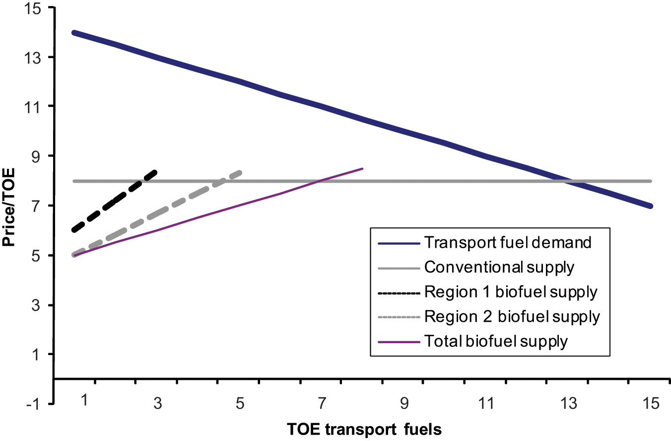
The market solution without a blending mandate

Note that the total sales of transport fuel only depend on T_C; that is, total sales are given where the transport fuel demand schedule crosses the conventional fuel supply curve. Adding the two supply curves for biofuels gives total biofuel supply for any transport fuel price. The sales of conventional fuel are then equal to the residual demand, which in Figure 1 for practical reasons are approximately half of the transport fuel demand. In 2004, biofuel sales in the European Union were about 2%, which had increased to about 3% in 2008.

Welfare and Environmental Costs

Global environmental damages D is a function of the stock of GHG in the atmosphere. Since we are looking at a fairly short period of time, we express damages as a function of the flow of GHG emissions by using a linear damage function $δ (ε_{1}^{C} + ε_{1}^{B} + ε_{2}^{B})$ , where the parameter δ is marginal environmental damage, $ε_{1}^{C}$ is emissions from conventional fuel consumption in Region 1, and $ε_{1}^{B} (ε_{2}^{C})$ are emissions from biofuel production in Region 1 Equation (2).⁹

Furthermore, we assume that Region 1 receives a share Ψ₁ of the damages with Ψ₁ < 1. The welfare of Region 1 is then given by

w_{1} = C S_{1} + π_{1} - ψ_{1} δ (ε_{1}^{C} + ε_{1}^{B} + ε_{2}^{B}) + T_{C} ε_{1}^{C} + T_{B} ε_{1}^{B} + t_{1} y_{2} - s_{1} y_{1},

(8)

where π₁ is the profit of the representative biofuels producer in Region 1, $T_{C} ε_{1}^{C}$ is income from taxing conventional fuels, $T_{B} ε_{1}^{B}$ is income from taxing emissions in biofuels production, t₁y₂ is income from the BCA on biofuel imports, and s₁y₁ is subsidy payments to local biofuel producers.

As mentioned, we measure GHG emissions in the same unit as transportation fuels. Total GHG emissions from the use of conventional fuels are then given by $ε_{1}^{C} = [\frac{M_{1} - T_{C}}{N_{1}} - y_{1} - y_{2}]$ . Emissions from the processing of biofuels ε^B_i in both regions are given from Equation 4, with abatement in Region 1 given by Equation 5.

For global welfare W, we have

W = w_{1} + π_{2} - (1 - ψ_{1}) δ (ε_{1}^{C} + ε_{1}^{B} + ε_{2}^{B}),

(9)

where π₂ is the profit of the representative biofuels producer in Region 2 and $(1 - Ψ_{1}) δ (ε_{1}^{C} + ε_{1}^{B} + ε_{2}^{B})$ are environmental damages in the rest of the world. Note that we need not consider consumer surplus in Region 2 since Region 2 also faces a completely elastic supply of conventional fuels.

Use of Trade Policies Without a Blending Mandate

BCA Only

Since Region 1 cannot enforce emission taxes in Region 2, the question is to what extent the BCA t₁ can improve global welfare. There is also a question of whether the subsidy to domestic production of biofuels s₁ or the environmental policy instruments T_C and T_B should be used in any way to limit emissions from biofuels production in Region 2. We start by looking at the most simple case without a blending mandate and without an import standard.

Producer surplus can simply be written as θ₁₁ (y₁)² and θ₂₂ (y₂)². These expressions can, together with Equations 2, 4, and 5, be inserted into the welfare functions (Equations 8 and 9), and after a great deal of rearranging we have for total welfare W

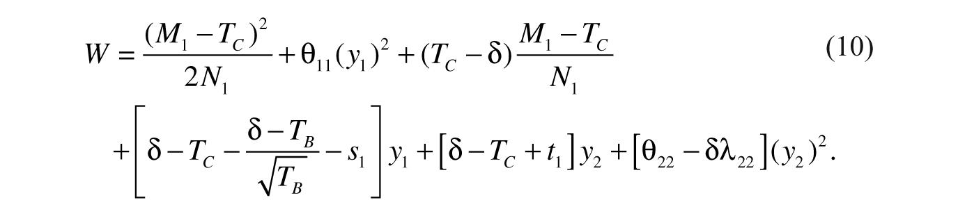
\begin{matrix} W = \frac{{(M_{1} - T_{C})}^{2}}{2 N_{1}} + θ_{11} {(y_{1})}^{2} + (T_{C} - δ) \frac{(M_{1} - T_{C})}{N_{1}} \\ + [δ - T_{C} - \frac{δ - T_{B}}{\sqrt{T_{B}}} - s_{1}] y_{1} + [δ - T_{C} + t_{1}] y_{2} + [θ_{22} - δ λ_{22}] {(y_{2})}^{2} . \end{matrix}

(10)

The first two terms in Equation 10 are consumer and producer surplus in Region 1, respectively. The third term is tax income minus the environmental damages from the use of conventional fuels. The fourth term is the external effects of Region 1 biofuel production; that is, domestic biofuel production reduces GHG emissions, decreases conventional fuel tax income, and leads to subsidy outlays. The fifth term is the gross effect of foreign biofuel production, which does not include emissions from the production in Region 2. These are included in the last term as a correction of the Region 2 producer surplus.

We maximize W with respect to T_C, t₁, s₁, and T_B. The first-order conditions are given by

\frac{\partial W}{\partial T_{C}} = - \frac{T_{C} - δ}{N_{1}} + [δ - T_{C} - \frac{δ - T_{B}}{\sqrt{T_{B}}} - s_{1}] \frac{1}{2 θ_{11}} = 0,

(11)

\frac{\partial W}{\partial t_{1}} = - [δ - T_{C} + t_{1}] + 2 δ λ_{22} y_{2} = 0,

(12)

\frac{\partial W}{\partial s_{1}} = [δ - T_{C} - \frac{δ - T_{B}}{\sqrt{T_{B}}} - s_{1}] = 0,

(13)

\frac{\partial W}{\partial T_{B}} = - [δ - T_{C} - \frac{δ - T_{B}}{\sqrt{T_{B}}} - s_{1}] \frac{1}{θ_{11}} + [\frac{δ - T_{B}}{T_{B}}] y_{1} = 0 .

(14)

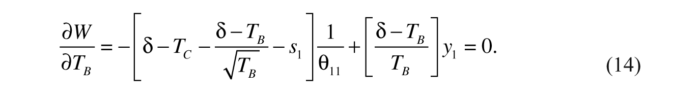
First, note that the optimal BCA t₁ is independent of the optimal subsidy s₁ and the GHG tax on domestic biofuel production T_B. Note also that the subsidy is independent of the BCA. Thus, the instrument used for regulating the supply of biofuels from Region 2 to Region 1 and the instruments used for regulating the domestic biofuels supply should be set independently of each other. In other words, policies should not be guided by intentions to “level the playing field.” The reason is the flat conventional fuel supply curve fixing the equilibrium price of transport fuels. Note that when Region 1 introduces a blending mandate, this independence disappears in spite of the flat conventional supply curve (see the section “Numerical Illustrations”).

The solution to the set of equations Equations 11, 12, 13, and 14 is T_C = δ, T_B = δ, s₁ = 0 and t₁=2δ₂₂y₂. The BCA is positive, and we can see that it equals the global marginal environmental damage from a marginal increase in imports. Our results are summarized in the following proposition:

Proposition 1: In a situation with import of biofuels from countries without a climate policy, global welfare can be improved by subjecting the import to a BCA, depending on the marginal environmental damage embodied in the last unit of output exported. Domestic biofuel production should be subject to the same GHG emission taxes as other sectors and should receive no production subsidies.

The BCA is increasing in the import volume. The understanding is that GHG emissions per unit of biofuel increases with output. Furthermore, as long as T_C = T_B = δ, that is, the environmental damage resulting from both conventional fuel use and domestic production of biofuels, is fully internalized, the subsidy to biofuels s₁ should be zero. On the other hand, if for instance T_B < δ, the subsidy should be negative.

The BCA does not give any incentive to invest in GHG abatement in Region 2. Thus, Region 1 is likely able to improve global welfare further by using more instruments. We will return to this in the section “Use of an Import Standard Together With a BCA.”

BCA With Point of Departure in Domestic Welfare

If Region 1 were free to set t₁ and s₁, it would not necessarily do so with the aim of maximizing global welfare. Many suspect that BCAs and subsidies will be misused. In order to investigate the scope of such misuse, we look at the optimal t₁ and s₁ when Region 1 only maximizes its own welfare given by Equation 8. The tax on conventional fuels and the domestic tax on biofuel production should then be according to T_c, T_B = Ψ₁δ. Thus, the welfare of Region 1 is given by

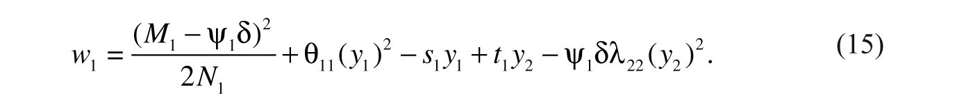
w_{1} = \frac{{(M_{1} - ψ_{1} δ)}^{2}}{2 N_{1}} + θ_{11} {(y_{1})}^{2} - s_{1} y_{1} + t_{1} y_{2} - ψ_{1} δ λ_{22} {(y_{2})}^{2} .

(15)

From the first-order condition for the optimal BCA, we obtain

t_{1} = 2 (ψ_{1} δ λ_{22} + θ_{22}) y_{2} .

(16)

There are two effects of the BCA; it will reduce emissions from biofuel production in Region 2, and it makes it possible for Region 1 to appropriate some of the producer surplus in Region 2 (beggar-thy-neighbor policy). Note that the difference between the unilateral BCA and the globally optimal BCA is given by [θ₂₂ − (1 − Ψ₁)δλ₂₂]2y₂. Defining misuse of BCA as setting a too high BCA, we obtain

Proposition 2: Region 1 will only misuse the BCA when θ₂₂ > (1 − Ψ₁)δλ₂₂.

Thus, misuse is less likely if the share of environmental damages belonging to Region 1 Ψ₁ decreases. Since Region 1 only partly internalizes the environmental damages from GHG emissions in Region 2, the emission-reduction part of the BCA is smaller than desirable. Thus, although Region 1 has an incentive to apply a beggar-thy-neighbor policy, the domestic second-best BCA may be close to the globally optimal BCA.

For the optimal subsidy, we have

\frac{\partial W}{\partial s_{1}} = - \frac{s_{1}}{2 θ_{1}} < 0 .

(17)

Again, we note that the optimal subsidy is zero. When T_C = T_B = Ψ₁δ, the environmental damage resulting from conventional fuel use and domestic production of biofuels is fully internalized. There is thus nothing to gain from increasing the use of biofuels any further by setting s₁ > 0.

Use of an Import Standard Together With a BCA

The European Union is considering an absolute standard for biofuel import, which would deny all biofuels not fulfilling the standard at the border. The European Union is also discussing a multicriteria standard, that is, specifying not only GHG emissions per unit of production but also working conditions in the biofuels industry and the effect of biofuels production on biodiversity conservation. In this article, we only consider a standard on GHG emissions per unit of output γ₁. To avoid the problem of shuffling, the standard would have to hold for the whole production of biofuels in Region 2, also the amount being used for domestic purposes. As noted previously, the emissions from the fixed supply of biofuels from the producers in Region 2 to the domestic Region 2 market is included in Equation 4. From Equation 4 it then follows that, in order to be able to export, the producer in Region 2 must buy abatement according to

λ_{22} y_{2} {(1 + A_{2})}^{- 1} = γ_{1} - λ_{2},

which directly yields the abatement cost function: $A_{2} = \frac{λ_{22}}{γ_{1 - λ_{2}}} y_{2} - 1$ . As given above, we skip the linear term in the emission function (λ₂ = 0), and the −1 term in the cost and profit functions as they do not affect the results. The cost function for the representative producer in Region 2 is then $c_{2} (y_{2}, γ) = \frac{λ_{22}}{γ_{1}} y_{2} + θ_{22} {(y_{2})}^{2}$ . Thus, the supply of Producer 2 is given by

y_{2} = \frac{T_{c} - λ_{22} / γ_{1} - t_{1}}{2 θ_{22}},

(18)

and the profit is still given by π₂ = θ₂₂(y₂)².

Again we consider global welfare. We know from above that global welfare is maximized when T_C and T_B is set equal to δ, and when s₁ is set equal to zero. The welfare-maxmizing import standard and the BCA is then found from

\max_{γ, t_{1}} {θ_{22} {(y_{2})}^{2} - δ γ_{1} y_{2} + t_{1} y_{2}},

where the first term is the profit of the foreign industry, the second term is environmental damage resulting from GHG emissions in Region 2 given the import standard γ₁, and the third term is income from the BCA. Note that, as long as T_C, T_B = δ and s₁ = 0, it is only the profit of the foreign industry and the emissions of the foreign industry that enter the maximum expression. Hence, when setting the standard, Region 1 should not look at the emissions of its own industry.

After inserting for y₂ and some rearranging, the two first-order conditions can be written as follows:

\frac{\partial W}{\partial γ_{1}} = [\frac{λ_{22}}{{(γ_{1})}^{2}} - δ] y_{2} + (t_{1} - δ γ_{1}) \frac{λ_{22}}{2 θ_{22} {(γ_{1})}^{2}} = 0,

(19)

\frac{\partial W}{\partial t_{1}} = δ γ_{1} - t_{1} = 0 .

(20)

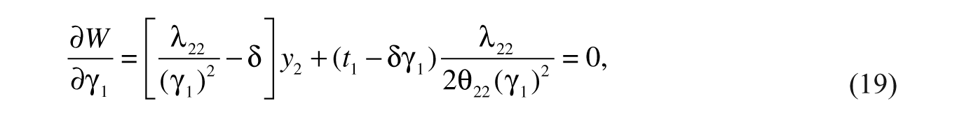
The optimal BCA given the standard is δγ₁. Inserting t₁ = δγ₁ into Equation 19 yields the optimal import standard: $γ_{1} = \sqrt{λ_{22}} / \sqrt{δ}$ , and by inserting the same into Equation 20, we find that the optimal BCA should be equal to $\sqrt{δ λ_{22}}$ . Since emissions per unit of output is now constant, the BCA is no longer dependent on import volume as in the case covered in subsection “BCA Only.” Finally, note that given T_B = δ, we know from the subsection “The Supply of Biofuels to Region 1” that emissions per unit of output from the biofuels industry in Region 1 is equal to $\sqrt{λ_{11}} / \sqrt{δ}$ . Hence, we have the following proposition:

Proposition 3: The welfare-maximizing import standard should be set such that the emissions per unit of output is as if the foreign producer were subject to an emission tax δ. Moreover, the BCA should be positive and equal to the marginal environmental damage from the last unit of output exported.

An import standard cannot replace a BCA fully. The reason is that the optimal import standard does not remove all emissions from the export of foreign biofuels, and since these residual emissions lead to environmental damages, they should be taxed in one way or another. Governments will seldom have enough information to set the correct import standard given by $γ_{1} = \sqrt{λ_{22}} / \sqrt{δ}$ . All the same, the principle that the standard should be set according to the hypothetical outcome of subjecting the foreign producer to an emission tax could be used to guide the setting of an import standard. For instance, the standard should be more stringent than the laissez faire emission intensity.

In fact, it can be shown that the combination of an import standard and the BCA will yield exactly the same GHG emissions, export output, and abatement level as in the case where it was possible for Region 1 to directly decide the abatement level in Region 2 in addition to setting a BCA. Thus, the import standard must improve global welfare. The reason is that it forces the biofuels industry in Region 2 to carry out profitable abatement investments.

Trade Policies With a Blending Mandate

Market Equilibrium

So far we have concluded that the taxes on GHG emissions T_C and T_B should not be distorted and that an import standard γ₁ improves welfare. We will use these insights in the analysis of a blending mandate.

A blending mandate fundamentally changes the way the market for transport fuels works. Earlier we had that the BCA should be set independently of the domestic production subsidy and vice versa (see Equations 12 and 13). The reason was that none of the instruments affected the price on conventional fuels. However, with a blending mandate the different policy measures will all depend on each other. In a way, the blending mandate creates a new product that we call transportation fuel and that must consist of biofuels and conventional fules in certain proportions.

Denote the blending mandate by η₁, and the supply of transportation fuel by Q, and observe that we must have η₁(y₁ + y₂)Q₁.¹⁰ Given the blending mandate, the cost of one unit of transport fuel is given by

(1 - η_{1}) T_{C} + η_{1} ρ_{1},

(21)

where ρ₁ is the Region 1 equilibrium price of biofuels. Since biofuels are guaranteed some sales, we may now have T_C < ρ₁. Furthermore, the equilibrium condition for the transport market in Region 1 is now P₁ = (1 − η₁)T_C + η₁ρ₁ (instead of P₁ = T_c).

By adding the two supply functions for biofuels given in Equations 7 and 18, and given that y₁ + y₂ = η₁Q₁, we obtain the following relationship between the biofuel price and total sales of transport fuel:

\frac{ρ_{1} + s_{1} - 2 \sqrt{T_{B}}}{2 θ_{11}} + \frac{ρ_{1} - λ_{22} / γ_{1} - t_{1}}{2 θ_{22}} = η_{1} Q_{1} .

(22)

This equation can be used to solve the equilibrium price of biofuels ρ₁ as a function of total supply of biofuels. Then by inserting ρ₁(Q₁) into Equation 21, and given that P₁ = (1 − η₁)T_C + η₁ρ₁, we obtain the supply of transport fuels:

P_{1} = \frac{2 θ_{11} θ_{22} {(η_{1})}^{2}}{θ_{11} + θ_{22}} Q_{1} + \frac{η_{1} θ_{11} (t_{1} + \frac{λ_{22}}{γ_{1}})}{θ_{11} + θ_{22}} + (1 - η_{1}) T_{C} - \frac{η_{1} θ_{22} (s_{1} - 2 \sqrt{T_{B}})}{θ_{11} + θ_{22}} .

(23)

First, note from the first term in Equation 23 that we now have an increasing supply curve for transportation fuels. The reason is of course the increasing marginal costs of biofuels. Note also from the last term in Equation 23 that a subsidy to domestic production of biofuels s₁ will shift the supply curve downwards and increase the supply of transportation fuels for any given price of transportation fuel. As this will also increase the use of conventional fuels, a subsidy to domestic production of biofuels s₁ works as an implicit subsidy to conventional fuels as pointed out by De Gorter and Just (2009). We can illustrate the market solution in the following diagram (Figure 2).

Figure 2.

The market solution with a blending mandate

Note that the total sales of transportation fuels no longer depend solely on T_C. From Equation 23 we see that the total sales of transport fuels now depend on all the instruments s₁, t₁, γ₁, and T_B in addition to T_C. Total sales are given where the transportation fuel demand schedule crosses the transportation fuel supply curve. As long as the blending mandate is binding and the other policy instruments are the same, this will happen to the left of the original equilibrium, that is, with lower total sales of transport fuel. Total biofuel supply is then equal to a η₁ share of total supply, and sales of conventional fuel is equal to a (1 − η₁) share of total supply.

Once we know the new market equilibrium Q₁, it is easy to calculate the respective market shares. The sales of conventional fuels is equal to (1 − η₁)Q₁, and the price of biofuels is given implicitly by Equation 22. This price can be inserted into Equations 7 and 18. We then obtain for the supply of biofuels

y_{1} = \frac{(s_{1} + t_{1} + \frac{λ_{22}}{γ_{1}} - 2 \sqrt{T_{B}}) N_{1} + 2 η_{1} θ_{22} [M_{1} + η_{1} (s_{1} - 2 \sqrt{T_{B}}) - (1 - η_{1}) T_{C}]}{Δ},

(24)

y_{2} = \frac{- (s_{1} + t_{1} + \frac{λ_{22}}{γ_{1}} - 2 \sqrt{T_{B}}) N_{1} + 2 η_{1} θ_{11} [M_{1} - η_{1} (t_{1} + \frac{λ_{22}}{γ_{1}}) - (1 - η_{1}) T_{C}]}{Δ},

(25)

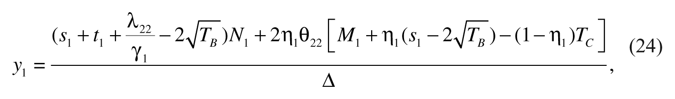
where Δ = 2(θ₁₁ + θ₂₂)N₁ + 4θ₁₁θ₂₂(η₁)².

Our conjectures above are easily verified: Given the blending mandate η₁, the instruments T_C, s₁, T_B, t₁, and γ₁ now have more wideranging trade effects. These are summarized in the following proposition:

Proposition 4: First, increasing t₁ and/or decreasing γ₁ not only reduces the import of biofuels but also spurs biofuel production in Region 1. Second, increasing s₁ and/or decreasing T_B not only spurs biofuel production in Region 1 but reduces the import of biofuels.

Policy makers should be aware of how a blending mandate changes the workings of the market. In the situation with a blending mandate, domestic producers of biofuels will have much to gain from convincing their goverment to set a strict import policy for foreign biofuels. Without a blending mandate, the incentive to try to influence import policy for biofuels disappears.

In the Appendix, we show that any binding blending mandate η₁ is equivalent to introducing an extra tax on conventional fuels T₁ and a general subsidy S₁ on all biofuels with the additional constraint that the income from the tax and the outlay for the subsidy should balance, that is, T₁(1 − η₁)Q₁ = S₁η₁Q₁.¹¹ Clearly, when the policy instruments T_C, T_B, s₁, t₁, and γ₁ are set as in the global first-best or second-best solution, any T₁, S₁ ≠ 0 must be nonoptimal. Hence, a binding blending mandate will likely decrease global welfare.

The BCA Given a Blending Mandate

We will now look at the optimal BCA with a blending mandate and an import standard in place. With T_C, T_B = δ, global welfare is given as

W = \frac{N_{1}}{2 {(η_{1})}^{2}} {(y_{1} + y_{2})}^{2} + θ_{11} {(y_{1})}^{2} + θ_{22} {(y_{2})}^{2} + t_{1} y_{2} - s_{1} y_{1} - δ γ_{1} y_{2},

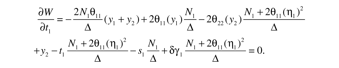
where the first term is consumer surplus, the second and third terms are producer surplus, the fourth and the fifth terms are BCA income and subsidy outlay, and, finally, the last term is environmental damage resulting from production in the other region.¹² The output quantities of biofuels y₁ and y₂ are given from Equations 24 and 25. Hence,for the derivatives we have $\frac{\partial y_{1}}{\partial t_{1}} = \frac{N_{1}}{Δ}$ and $\frac{\partial y_{2}}{\partial t_{1}} = \frac{- N_{1} - 2 θ_{11} {(η_{1})}^{2}}{Δ}$ . The first-order condition is then

\begin{array}{l} \frac{\partial W}{\partial t_{1}} = - \frac{2 N_{1} θ_{11}}{Δ} (y_{1} + y_{2}) + 2 θ_{11} (y_{1}) \frac{N_{1}}{Δ} - 2 θ_{22} (y_{2}) \frac{N_{1} + 2 θ_{11} {(η_{1})}^{2}}{Δ} \\ + y_{2} - t_{1} \frac{N_{1} + 2 θ_{11} {(η_{1})}^{2}}{Δ} - s_{1} \frac{N_{1}}{Δ} + δ γ_{1} \frac{N_{1} + 2 θ_{11} {(η_{1})}^{2}}{Δ} = 0 . \end{array}

The first four terms cancel. Hence, simplifying yields

(δ γ_{1} - t_{1}) \frac{N_{1} + 2 θ_{11} {(η_{1})}^{2}}{Δ} = s_{1} \frac{N_{1}}{Δ} .

(26)

In the global first-best, we had $t_{1}^{*} = δ γ_{1}$ (see Equation 20). Thus, we have the following proposition:

Proposition 5: The rule for setting the BCA now includes the subsidy rate s₁. The BCA should be lower, if the subsidy rate is higher.

The blending mandate does not rule out a BCA. However, if subsidies to domestic biofuel production are extensive, the BCA could turn negative.

Numerical Illustration

To illustrate the effects of a blending mandate, we have calibrated the model to data from 2004 (Table 1) covering the EU transport market, the European production of biofuels, and the Brazilian ethanol production (see Eurostat, 2007; Kutas, Lindberg, & Steenblik, 2007). Since our focus is on the blending mandate and the data with respect to GHG abatement possibilities are limited, we did not include possibilities for GHG abatement in biofuel production and, consequently, we cannot analyze the effect of an import standard.¹³

Table 1.

Key Data for the Year 2004

Description	Price in euro or %
Price conventional fuels	1.07 euro/liter
Excise tax conventional fuel	0.70 euro/liter
Carbon tax conventional fuel	0.05 euro/liter
International price conventional fuel	0.32 euro/liter
Marginal cost EU biofuels	0.56 euro/liter
Unit subsidy EU biofuels	0.31 euro/liter
Marginal cost Brazilian ethanol	0.26 euro/liter^a
Tariff Brazilian ethanol	0.19 euro/liter
Net GHG reduction EU biofuels	50%
Net GHG reduction Brazilian ethanol	85%

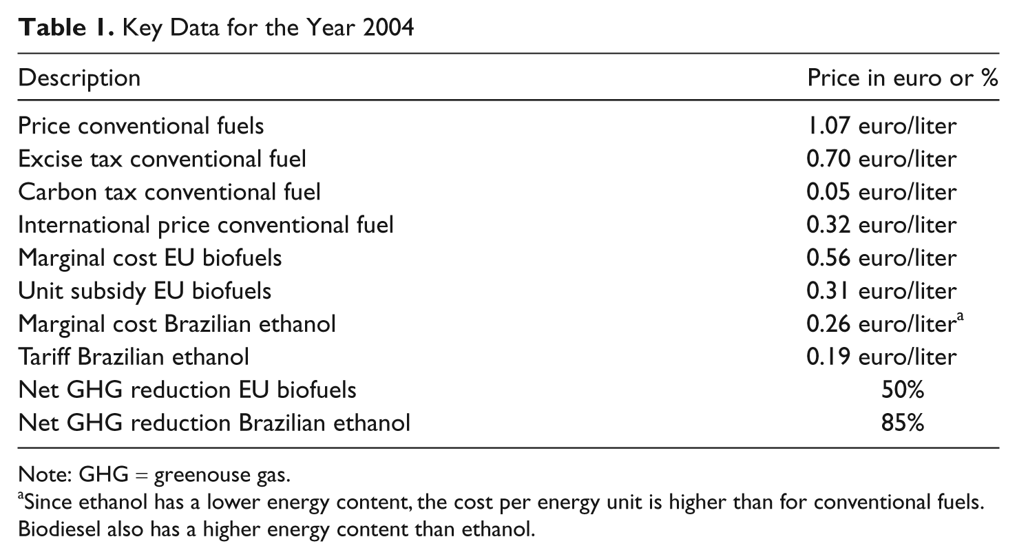
Note: GHG = greenouse gas.

Since ethanol has a lower energy content, the cost per energy unit is higher than for conventional fuels. Biodiesel also has a higher energy content than ethanol.

We treat the European Union as one market and convert all fuels to energy equivalents. By weighting consumer prices for gasoline and diesel in each country by their share of total consumption, we computed an average consumer price, excise tax, and carbon tax for conventional fuels. Supply of conventional fuels is then assumed to be completely elastic at the average consumer price. Given a price elasticity of transport fuels of −0.4, it is then easy to fit a linear demand schedule to the 2004 data.

Supply of Brazilian ethanol is upward sloping, and the average cost is assumed to increase by 5% for every doubling. In 2004, the production costs were comparable to the international price of gasoline measured in volume units (Kojima et al., 2007). Then by using production figures from 2004, we were able to calibrate the Brazilian supply schedule.

We decided to treat European biodiesel and ethanol together. Due to the intricate support scheme for European biofuel production, it is difficult to find cost data. Instead, we used the cost of producing biodiesel from soybeans, which is available from the U.S. energy department. Moreover, for European biofuel production, we assumed that the average cost increases by 10% for every doubling due to less availability of land. The supply schedule can then be calibrated using current biofuels production in the European Union. Finally, the current European subsidy to biofuels production measured as a fixed per-unit subsidy is calculated residually.¹⁴

The carbon tax amounts to 20 euro/metric ton CO₂. Domestic biofuels are partly exempt from the excise tax, which is reflected in the subsidy.

In what follows, we show results for three scenarios. In the baseline scenario, we introduce a 5.75% blending mandate based on the 2004 figures. The implicit tax on conventional fuels and subsidy to both types of biofuels can then be calculated. In the next scenario, we look at the optimal tariff from a global point of view, given the EU domestic biofuel subsidy. Finally, we look at the optimal combination of the EU subsidy and tariff.

In the baseline scenario, total subsidies to European biofuels production amounts to 8 billion euro, of which more than half is paid directly by consumers through a higher price on transport fuels. Consumers also subsidize Brazilian ethanol through the blending mandate, and this subsidy amounts to nearly 4 billion euro. Thus, given current policy, the blending mandate implies a transfer of more than 8 billion euro from consumers to biofuel producers, which does not show up in the national budgets.

The tariff is nonoptimal both from a global point of view and from a strict EU perspective. If for some reason the EU cannot remove the European domestic biofuel subsidy, tariffs should be negative as indicated in the third row of Table 2. The blending mandate is then reached by increasing only the Brazilian ethanol supply and keeping the EU biofuels supply fixed. The welfare improvement from such a policy shift is about 3 billion euro for the European Union alone. Finally, the hidden transfer from consumers to biofuels producers is eliminated.

Table 2.

The Effect of Introducing a 5.75% Blending Mandate

Scenarios	EU biodiesel subsidy	Ethanol tariff	Implicit tax	Implicit subsidy
Baseline	0.31	0.19	0.02	0.32
Optimal tariff	0.31	−0.1	0	0
Optimal subsidy + tariff	0	0.03	0.01	0.12

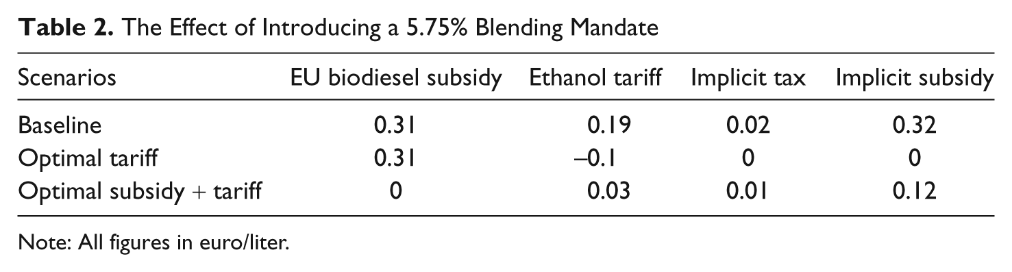
Note: All figures in euro/liter.

From a global welfare point of view, the European domestic biofuel subsidy should be completely removed and the tariff set slightly positive. The reason for not removing the tariff fully is the small, but still significant, GHG emissions from Brazilian ethanol production. Finally, note that the optimal policy does not eliminate the hidden subsidies. Removing the domestic subsidy implies that in order to reach the blending mandate, approximately 4 billion euro must be transferred from EU consumers to Brazilian biofuel producers. This is also optimal from an EU point of view.

Discussion and Conclusion

In this article, we study trade policies for biofuels in the context of reducing GHG emissions. The global interest in biofuels is also driven by concern for energy safety and local environmental pollution, particularly in developing countries, as well as by an interest in supporting domestic agriculture related to ongoing trade liberalizing negotiations (Kojima et al., 2007). The current EU policies for biofuels are likely influenced by all of these factors with the possible exception of concern for local environmental pollution.

For an incomplete international climate agreement, BCA can be used to prevent leakage when signatory and nonsignatory countries are trading. Due to the scope for misuse, allowing individual regions to decide BCA levels may jeopardize the international trading system. Rather, setting BCAs to reduce carbon leakage should follow a fixed scheme negotiated and agreed upon by the partners of future climate treaties. It should also be considered whether the countries introducing GHG emission–based BCAs should be the recipient of the income from the BCAs. Furthermore, BCAs and standards may be questioned within the WTO/GATT rules. De Gorter and Just (2010) forcefully argue that standards are illegal under WTO law. Horn and Mavroidis (2009), on the other hand, hold that a BCA will be considered domestic and not a trade instrument. Furthermore, following the WTO Appellate Body Report on the Dominican Republic—Import and Sale of Cigarettes, even if the government wants to both protect domestic producers and the environment, using a BCA may pass if it can be proved that it is actually protecting the environment.

The European Union is planning to introduce a standard for biofuel imports. Our results indicate that import standards combined with BCAs can improve global welfare. However, our results depend on the costs of successful enforcement.

The EU is also toughening its biofuel blending mandate. We show that a blending mandate fundamentally alters the way the market works. For instance, if domestic biofuel production is subsidized, the optimal BCA may be negative. Clearly, a negative BCA is unrealistic, yet on the other hand, it stresses the need for the European Union to reconsider both its trade policy and subsidy policy with respect to biofuels.

Using 2004 data for the EU, we find that a 5.75% blending mandate implies a transfer of 8 billion euro from consumers to producers . This should not be misinterpreted as a welfare loss since the transfer partly shows up as increased producer surplus. Although our numerical model should not be expected to give exact figures, one may ask whether transferring anything in the range of this amount of money to biofuel suppliers is well spent given all the uncertainty regarding biofuels as a long-term solution to GHG abatement in the transport sector. Kutas et al. estimated the costs to achieve GHG reductions with current subsidies to be in the range of 215 to 800 per metric ton of CO₂-equivalent reduction, which can be contrasted to social cost of carbon estimates of 10 and 30 per ton emitted CO₂ (Kopp, Golub, Keohane, & Onda, 2011; Tol, 2008). Market prices for emission permits in 2006 at the Chicago and the European Climate Exchange were in the range of 3 to 26 (Kutas et al., 2007). Hence, we feel it is safe to claim that the current EU biofuel policy does not achieve the biggest “bang for the buck.”

Policies for reducing emissions from the transport sector are easily combined with other targets. Both industrialized countries and developing countries are concerned about energy safety. If energy safety is another objective of EU’s biofuels policy, the current tariff on ethanol imports from, for example, Brazil, could be suboptimal. Ethanol from Brazil would reduce dependence on both Russian gas and oil from OPEC, but it is also superior in terms of GHG reductions compared to EU-produced ethanol (Kojima et al., 2007), indicating that the optimal tariff in this case would be negative. The empirical application part of this study has focused on the European Union, but the U.S. policies bear a lot of resemblance. “The modern U.S. ethanol industry was born subsidized,” Koplow and Steenblik (2008) write, finding the 18.5 billion liters of ethanol produced in the United States during 2006 to be subsidized by about 4 billion.

Clearly, the current EU policy on biofuels is hard to grasp within our model. One additional argument frequently cited for subsidies is the potential for future cost reductions using new cleaner energy technologies (see Hamelinck & Faaij, 2006). Here, we have not treated induced technological change, which is clearly an area for future research.

Footnotes

Appendix

Acknowledgements

We thank two anonymous referees for valuable comments. Remarks and suggestions from colleagues in the research program ENTWINED are also appreciated.

The authors declared no potential conflicts of interest with respect to the research, authorship, and/or publication of this article.

The authors disclosed receipt of the following financial support for the research, authorship, and/or publication of this article: We are grateful for financial support from the ENTWINED programme, which is funded by the Mistra Foundation. We also acknowledge financial support from the Norwegian Research Council and Formas through the program Human Cooperation to Manage Natural Resources (COMMONS).

Notes

Håkan Eggert is Associate Professor in Economics at University of Gothenburg, Sweden. He is affiliated with the Statistics Norway as a part-time researcher. He earned his Ph.D. in economics from the University of Gothenburg in 2001 with a thesis on problems related to commercial fisheries. He has published papers on bioeconomics, risk, production, compliance, valuation and trade usually with a link to natural resources.

Mads Greaker heads the research group for energy economics at Statistics Norway in Oslo. He is affiliated with the Department of Economics, University of Gothenburg, Sweden, in a part-time capacity. He earned his Ph.D. in economics from the University of Oslo in 2002 with a thesis on the relationship between environmental policy and trade. He has published papers on the Porter-hypothesis, eco-labeling, as well as the economics of climate change.

References

Böhringer

Rosendahl

K. E.

(2010). Green promotes the dirtiest: On the interaction between black and green quotas in energy markets. Journal of Regulatory Economics, 37(3), 316-325.

Bushnell

Peterman

Wolfram

(2008). Local solutions to global problems: Climate change policies and regulatory jurisdiction. Review of Environmental Economics and Policy, 2(2), 175-193.

Chow

Kopp

R. J.

Portney

P. R.

(2003). Energy resources and global development. Science, 302, 1528-1531.

De Gorter

Just

D. R.

(2009). The economics of a blend mandate for biofuels. American Journal of Agricultural Economics, 91(3), 738-750.

De Gorter

Just

D. R.

(2010). The social costs and benefits of biofuels: The intersection of environmental, energy and agricultural policy. Applied Economic Perspectives and Policy, 32(1), 4-32.

European Commission. (2003). Directive 2003/30/EC of the European Parliament and of the Council of 8 May 2003 on the promotion of the use of biofuels or other renewable fuels for transport. Retrieved from http://ec.europa.eu/energy/res/legislation/doc/biofuels/en_final.pdf

European Environment Agency. (2006). Annual European Community greenhouse gas inventory 1990-2004 and inventory report 2006 (Technical Report No. 6/2006). Retrieved from http://reports.eeaeuropa.eu/technical_report_2006_6/en/.

Eurostat. (2007). Energy consumption and the environment. Luxembourg: Author.

Fargione

Hill

Tilman

Polasky

Hawthorne

(2008). Land clearing and the biofuel carbon debt. Science, 319, 1235-1238.

10.

Hamelinck

C. N.

Faaij

A. P. C.

(2006). Outlook for advanced biofuels. Energy Policy, 34, 3268-3283.

11.

Hoel

(1996). Should a carbon tax be differentiated across sectors? Journal of Public Economics, 59, 17-32.

12.

Horn

Mavroidis

P. C.

(2009). Burden of proof in environmental disputes in the WTO: Legal aspects. European Energy and Environmental Law Review, 18(2), 112-140.

13.

Intergovernmental Panel on Climate Change. (2007). Summary for policymakers. In Solomon

Qin

Manning

Chen

Marquis

Averyt

K. B.

. . . Miller

H. L.

(Eds.), Climate change 2007: The physical science basis (Contribution of Working Group I to the Fourth Assessment Report of the Intergovernmental Panel on Climate Change, pp. 1-18). Cambridge, UK: Cambridge University Press.

14.

Kojima

Mitchell

Ward

(2007). Considering trade policies for liquid biofuels. Washington, DC: World Bank ((Energy Sector Management Assistance Program [ESPM]).

15.

Koplow

Steenblik

(2008). Subsidies to ethanol in the United States. In Pimentel

(Ed.), Biofuels, solar and wind as renewable energy systems benefits and risks (pp. 79-108). New York, NY: Springer.

16.

Kopp

R. E.

Golub

Keohane

N. O.

Onda

(2011). The influence of the specification of climate change damages on the social cost of carbon (Economics Discussion Papers, No. 2011-22). Kiel, Germany: Kiel Institute for the World Economy. Retrieved from http://www.economics-ejournal.org/economics/discussionpapers/2011-22

17.

Kutas

Lindberg

Steenblik

(2007). Biofuels at what costs—Government support for ethanol and biodiesel in the European Union? London: Global Subsidies Initiativ/International Institute for Sustainable Development.

18.

Lapola

D. M.

Schaldach

Alcamo

Bondeau

Koch

Koelking

Priess

J. A.

(2010). Indirect land-use changes can overcome carbon savings from biofuels in Brazil. PNAS, 107 (8), 3388-3393.

19.

Macedo

I. C.

Seabra

J. E. A.

Silva

J. E. A. R.

(2008). Green house gas emissions in the production and use of ethanol from sugarcane in Brazil: The 2005/2006 averages and a prediction for 2020. Biomass and Energy, 32, 582-595.

20.

Maestad

(1998). On the efficiency of green trade policy. Environmental and Resource Economics, 11, 1-18.

21.

Maestad

(2001). Efficient climate policy with internationally mobile firms. Environmental and Resource Economics, 19, 267-284.

22.

Moschini

Lapan

Cui

Cooper

(2010). Assessing the welfare effects of US biofuel policies. AgBioForum, 13(4), 370-374.

23.

Oreskes

(2004). Beyond the ivory tower—The scientific consensus on climate change. Science, 306, 1686.

24.

Renewable Energy Roadmap. (2006). Renewable energy road map: Renewable energies in the 21st century: Building a more sustainable future (COM 2006, 848 final). Retrieved from http://ec.europa.eu/energy/ energy_policy/doc/ 03_renewable_energy_roadmap_en.pdf

25.

Searchinger

Heimlich

Houghton

R. A.

Dong

Elobeid

Fabiosa

. . . Yu

T.-H.

(2008). Use of U.S. croplands for biofuels increases greenhouse gases through emissions from land-use change. Science, 319, 1238-1241.

26.

Tol

R. S. J.

(2008). The social cost of carbon: Trends, outliers and catastrophes. Economics: The Open-Access, Open-Assessment E-Journal, 2, 2008-2025.

27.

United Nations Framework Convention on Climate Change. (2009, January 15). Executive Secretary speech to the Ministerial Conference on Global Environment and Energy in Transport, Tokyo, Japan. New York, NY: Author.