
Abstract
The State–Trait Inventory of Cognitive and Somatic Anxiety (STICSA) is a commonly administered self-report instrument of state–trait cognitive and somatic anxiety. Extant research has consistently supported the intended oblique two-factor scoring structure for the STICSA. However, this model assumes that population-level data have (or approximate) a simple structure and that item-level variance is unidimensional. These assumptions may not be tenable and have unintended consequences for STICSA subscore interpretation. Consequently, we tested these assumptions by fitting confirmatory and exploratory structural equation models to STICSA scores for a diverse sample of college students enrolled at a large Southwestern university in the United States (n = 635). Results indicated that cognitive and somatic factors are not equally robust and that STICSA items appear to measure a nonnegligible mixture of both latent cognitive and somatic anxiety. It is recommended that future research use exploratory structural equation model in tandem with CFA to directly model data complexity.
Keywords
The enduring distinction between anxiety as a temporary affective state in response to situational cues and anxiety as a personality trait has been traced as far back as Cicero (BCE; as cited in Lewis, 1970). However, Spielberger (1966) is often cited as introducing the first cohesive model of state–trait anxiety. Spielberger’s (1966, 1985) model of state–trait anxiety assumes that anxiety is unidimensional, but multifaceted, consisting of state and trait facets. According to the model, state anxiety is a transitory emotion characterized by a blend of cognitive (e.g., worry) and somatic symptoms (e.g., physiological arousal), whereas trait anxiety is characterized by a tendency to respond to environmental stimuli with elevated state anxiety. Spielberger’s refinement of the state–trait distinction (especially regarding the definition of trait anxiety as a behavioral predisposition) was initially widely adopted. However, his state–trait anxiety model was later criticized for its treatment of anxiety as unidimensional (e.g., Calvo et al., 2003; Endler & Kocovski, 2001).
There remains little consensus with respect to the nature and number of dimensions that underlie state–trait anxiety. Nevertheless, researchers tend to agree that cognitive and somatic symptoms warrant individual attention (e.g., Balyan et al., 2016; Clark & Watson, 1991; Endler & Kocovski, 2001; Martyn & Brymer, 2014). This led Ree et al. (2000) to develop the State–Trait Inventory of Cognitive and Somatic Anxiety (STICSA; Ree et al., 2000; Ree et al., 2008), initially published (with permission) by Grös et al. (2007), in order to facilitate direct comparisons of cognitive and somatic anxiety between state and trait facets.
Published empirical studies of the psychometric properties of the STICSA are growing in number (Grös et al., 2007; Lancaster et al., 2015; Ree et al., 2008; Roberts et al., 2016) in addition to research establishing STICSA cut-scores for identifying probable anxiety disorders (Van Dam et al., 2013), research establishing convergence of symptoms between self-ratings and ratings from an informant-adapted version of the scale (Grös et al., 2010; Grös et al., 2013), research on the psychometric properties of the scale translated into Italian (Balsamo et al., 2015; Carlucci et al., 2018), and the development of an adaptation of the scale for use with children (Deacy et al., 2016). Moreover, use of the STICSA in research is increasing exponentially. A Google Scholar search conducted at the time this article was written indicated approximately 50 peer-reviewed published journal articles using the STICSA to measure cognitive and somatic dimensions of state–trait anxiety, the vast majority of which were published in the past 5 years.
Preliminary findings for the reliability and validity of STICSA score interpretations are generally positive (Elwood et al., 2012). However, many crucial questions remain unresolved regarding the dimensionality of the scale that have important implications for how STICSA scores should be interpreted. A comprehensive review of what is currently known regarding the dimensionality of the STICSA is included in the section below, followed by a discussion of the requisite evidence that is needed to fill this gap in the literature.
Evidence of Dimensionality for STICSA Scores
Oblique Two-Factor Model
There is considerable empirical support for the oblique two-factor model as the best explanation for STICSA scores (Carlucci et al., 2018; Grös et al., 2010; Ree et al., 2008; Roberts et al., 2016) with few exceptions (Carlucci et al., 2018; Lancaster et al., 2015). Ree et al. conducted confirmatory factor analysis (CFA) on the screened STICSA item pool with a large Australian community sample (n = 576) of high school seniors, staff from local businesses, and academic and general staff at a nearby Australian university (Ree et al., 2000; Ree et al., 2008). Ree et al. conducted CFA on the state and trait forms, separately, to compare the fit of three competing factor models: (a) a one-factor model in which all items loaded onto a single factor (see Figure 1, Models 1 and 5), (b) an orthogonal two-factor model in which items written to assess symptoms of cognitive anxiety loaded onto a cognitive factor and items written to assess symptoms of somatic anxiety loaded onto a somatic factor (see Figure 1, Models 2 and 6), and (c) an oblique version of the orthogonal two-factor model (see Figure 1, Models 3 and 7). Items with cross loadings (
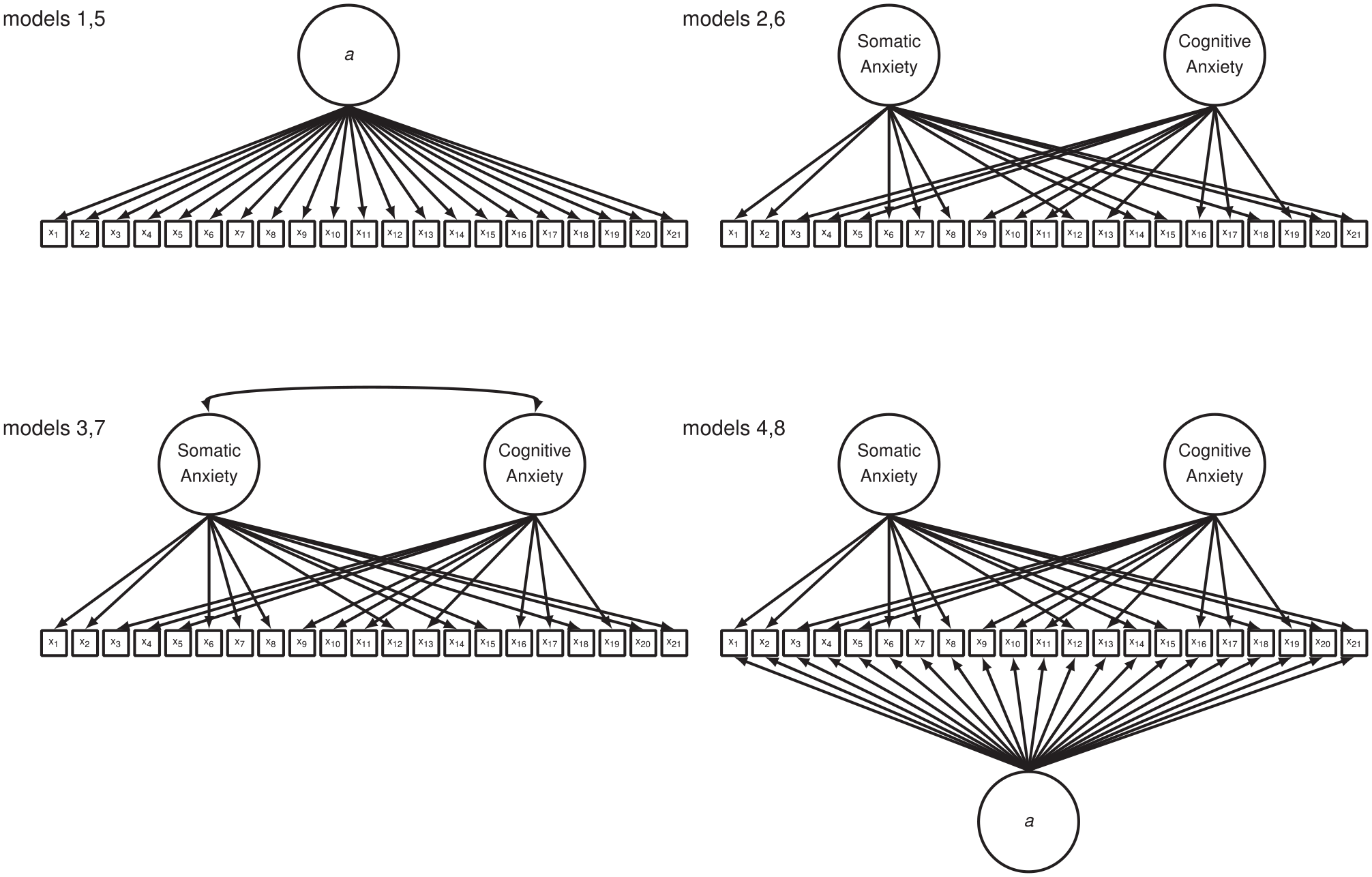
One-factor (Models 1 and 5), orthogonal two-factor (Models 2 and 6), oblique two-factor (Models 3 and 7), and bifactor (Models 4 and 8) path models tested with each STICSA form separately.
Grös et al. (2010) found support for the oblique two-factor model of the STICSA-Trait when compared with the one-factor model in a small sample of undergraduate psychology students (n = 146) enrolled at a large Northeastern university in the United States; and, they reported that the oblique two-factor model exhibited metric invariance across self-report and peer-informant–report versions of the scale. Roberts et al. (2016) also found support for the oblique two-factor model for both forms of the STICSA in a diverse sample of Canadian undergraduate students (n = 560). In addition, Carlucci et al. (2018) found support for the oblique two-factor model with a large Italian sample composed of a mixture of adults who responded to advertisements posted in established community centers and undergraduate students (n = 2,983) when compared with models tested by Ree et al. (2008) and others who conducted CFA on both forms of the STICSA together, as discussed in detail later (Balsamo et al., 2015; Grös et al., 2007; Roberts et al., 2016). Carlucci et al. also established scalar invariance for the oblique two-factor model across gender for both forms of the STICSA and across age (18-25, 26-50, and 51-99 years old) for the STICSA-State. However, factor loadings for three items (10 = “I can’t get some thought out of my mind,” 11 = “I have trouble remembering things,” and 20 = “I have butterflies in the stomach”) on the STICSA-Trait were variant between Italian middle-aged and older adults (26-50 and 51-99 years old). Consequently, only configural invariance was established for the STICSA-Trait across the three age groups investigated.
Lancaster et al. (2015) reported that the oblique two-factor model did not adequately fit STICSA-State or STICSA-Trait scores for separate samples of Black (n = 165) and White (n = 165) undergraduate students who were enrolled at a rural public Midwestern university in the United States. Nevertheless, they proceeded to conduct multigroup CFA in order to determine the degree to which the oblique two-factor model was invariant across these two racial groups. Lancaster et al.’s rationale was that results of psychometric studies of other anxiety scales (i.e., Anxiety Sensitivity Index: Silverman et al., 1991; Beck Anxiety Inventory: Beck & Steer, 1990; Fear of Negative Evaluation: Watson & Friend, 1969; Multidimensional Anxiety Scale for Children: March et al., 1997; Social Avoidance and Distress Scale: Watson & Friend, 1969) have suggested that scores obtained from White and Black individuals should not be compared because the underlying factor models are noninvariant (Chapman et al., 2009; Kingery et al., 2009; Lambert et al., 2004; Melka et al., 2010). They also cited research suggesting that Black individuals may experience more somatic symptoms than cognitive symptoms when compared with White individuals (Neal & Turner, 1991); and, they indicated that this may be particularly problematic for the STICSA given that it was designed with the intention of measuring both cognitive and somatic anxiety. Results indicated that the configural model did not adequately fit their data set. Unfortunately, Lancaster et al.’s (2015) study was grossly underpowered (n < 200) along with all but one of the factor analytic studies they reviewed to support their analyses with sample sizes ranging from 100 to 144 per group across studies (Chapman et al., 2009; Kingery et al., 2009; Lambert et al., 2004). Consequently, results of their study should be interpreted cautiously.
Oblique Four-Factor Model
STICSA-State and STICSA-Trait items have also been modeled together in CFA in order to determine the degree to which STICSA scores differentiate between state and trait facets of cognitive and somatic anxiety. Grös et al. (2007) conducted CFA on the combined forms with a Canadian community sample (n = 567) of psychiatric outpatients with anxiety or anxiety-related disorders and a sample of undergraduate psychology students who were enrolled at a large public Northeastern university in the United States (n = 311): (a) a one-factor model in which all items from both the STICSA-State and STICSA-Trait loaded onto a single factor (see Figure 2, Model 9), (b) an oblique two-factor model in which all STICSA-State and STICSA-Trait cognitive items loaded onto a cognitive factor and all STICSA-State and STICSA-Trait somatic items loaded onto a somatic factor (see Figure 3, Model 12), (c) an oblique two-factor model in which all STICSA-State items loaded onto a state factor and all STICSA-Trait items loaded onto a trait factor (similar to Figure 2, Model 11), and (d) an oblique four-factor model with state-cognitive, state-somatic, trait-cognitive, and trait-somatic factors (similar to Figure 3, Model 13). The oblique four-factor model provided an adequate to good fit to their sample data set and the fit was superior when compared with the fit of the remaining three competing models. In addition, Grös et al. reported that results of multigroup CFA indicated that this model exhibited metric invariance across the psychiatric outpatient and undergraduate student participant groups.
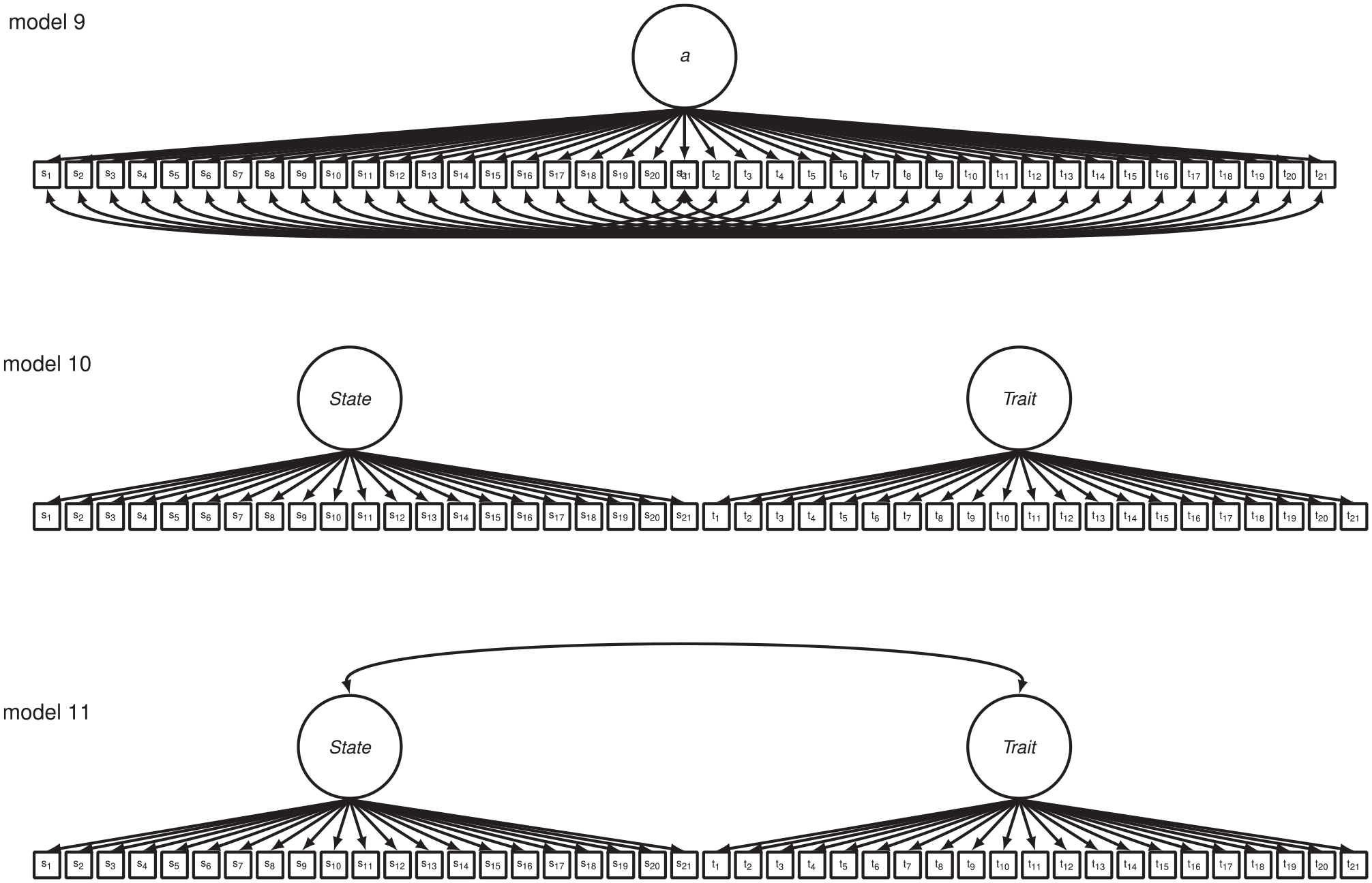
One-factor (Model 9), orthogonal two-factor state–trait (Model 10), and oblique two-factor state–trait (Model 11) path models of the STICSA-State and STICSA-Trait combined forms tested in the present study.
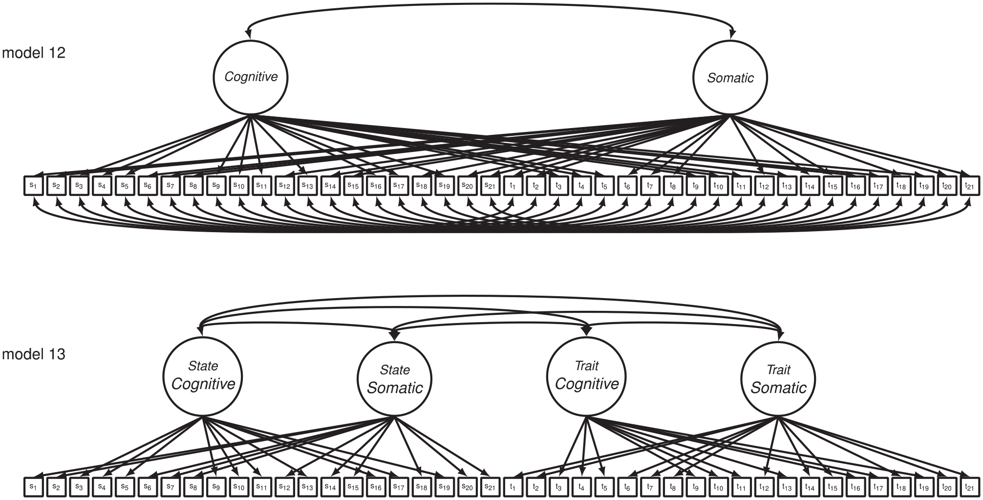
Oblique two-factor cognitive–somatic (Model 12) and oblique four-factor (Model 13) path models of the STICSA-State and STICSA-Trait combined forms tested in the present study.
However, Grös et al. (2007) correlated the residuals for identical items across the STICSA-State and STICSA-Trait both within (i.e., as in the one-factor model and the oblique two-factor cognitive–somatic model) and across factors (i.e., as in the oblique two-factor state–trait model and the oblique four-factor model). It may be justifiable to correlate error terms a priori for identical STICSA-State and STICSA-Trait items within factors (assuming
Higher Order and Bifactor Models
Roberts et al. (2016) noted that the four factors (state-cognitive, state-somatic, trait-cognitive, and trait-somatic) were highly correlated (r = .45-.84) in the oblique four-factor model tested by Grös et al. (2007). As a result, they also fit a higher order model consisting of the four first-order state-cognitive, state-somatic, trait-cognitive, and trait-somatic factors and a second-order superordinate general factor of anxiety (see Figure 4, Model 14) to data from the combined STICSA forms. The higher order model provided an equally adequate fit when compared with the oblique four-factor model. However, Carlucci et al. (2018) reported that this higher order model did not provide an adequate fit to their large Italian community/undergraduate student sample.
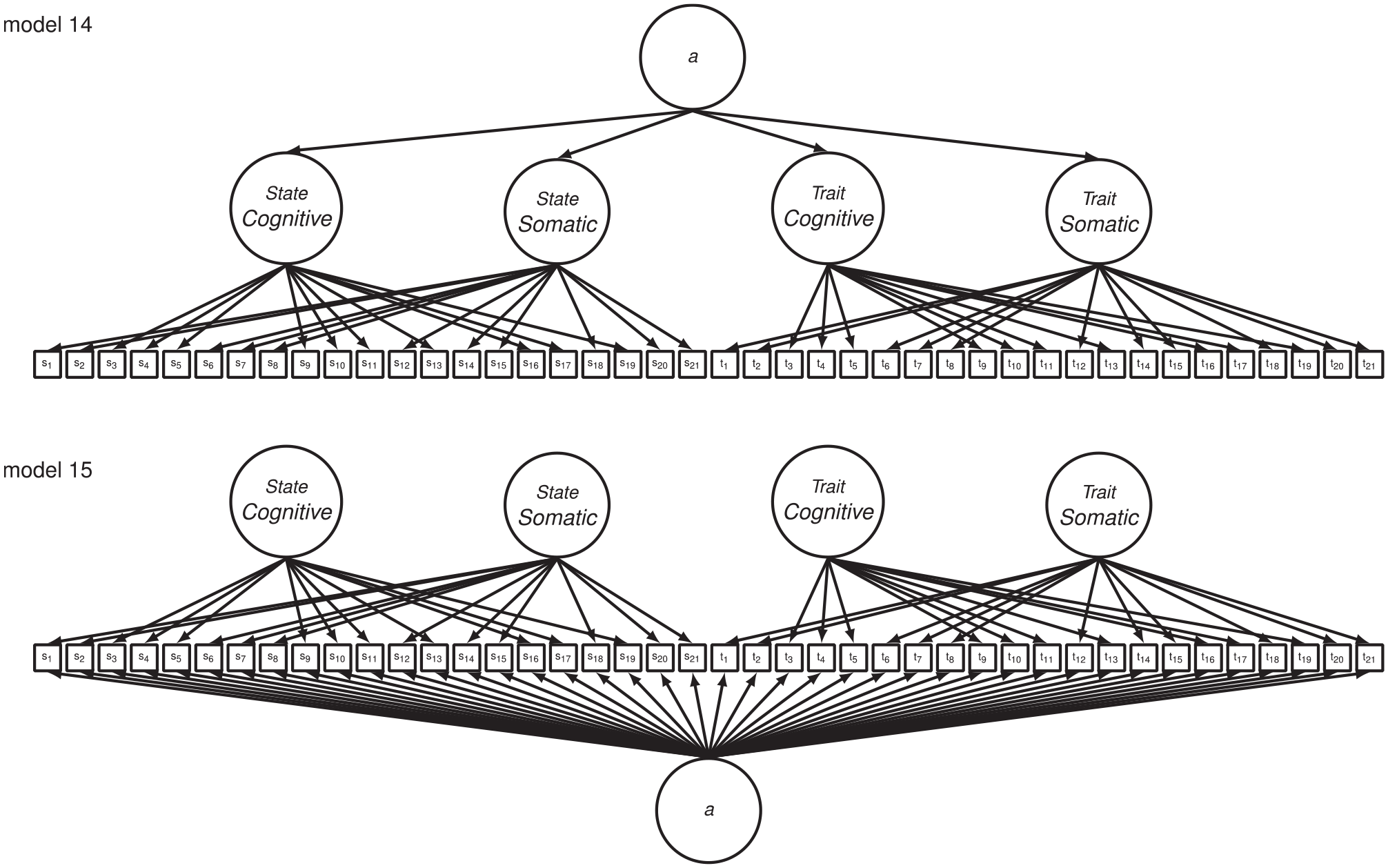
Higher order (Model 14) and bifactor (Model 15) models of the STICSA-State and STICSA-Trait combined forms tested in the present study.
Carlucci et al. (2018) also pointed out that no prior study had applied bifactor models to STICSA scores in order to disentangle shared variance due to general and group factors. Accordingly, they fit a series of bifactor models to their data set in addition to all of the models that had been proposed in the research at that time: (a) the oblique two-factor model proposed by Ree et al. (2008) for the state and trait forms of the STICSA modeled separately; (b) all four models proposed by Grös et al. (2007) for the state and trait forms of the STICSA modeled together, albeit with correlated residuals only applied a priori to identical STICSA-State and STICSA-Trait items that loaded onto the same factor (i.e., as in the one-factor model and the oblique two-factor cognitive–somatic model); (c) an orthogonal two-factor state–trait model for the combined state and trait forms in which all STICSA-State items loaded onto a state factor and all STICSA-Trait items loaded onto a trait factor; (d) a bifactor model with two group factors (cognitive and somatic) and a general anxiety breadth factor for the state and trait forms of the STICSA modeled separately (see Figure 1, Models 4 and 8); and (e) a bifactor model with four group factors (state-cognitive, state-somatic, trait-cognitive, and trait-somatic) and a general anxiety breadth factor for the state and trait forms of the STICSA modeled together (see Figure 4, Model 15). Findings from Carlucci et al. supported the oblique two-factor model for the STICSA-State and STICSA-Trait forms, modeled separately, as previously noted; and, they reported that none of the other competing models adequately fit their data set.
Unresolved Issues Regarding STICSA Score Interpretation
Table 1 tabulates all factor models of STICSA scores that have been proposed and tested to date. It is evident from the table that there is near uniform support for the oblique two-factor model when STICSA-State and STICSA-Trait scores are modeled separately (Carlucci et al., 2018; Grös et al., 2010; Ree et al., 2008; Roberts et al., 2016). Yet a few unresolved issues remain.
All Factor Models Proposed for STICSA Scores to Date.
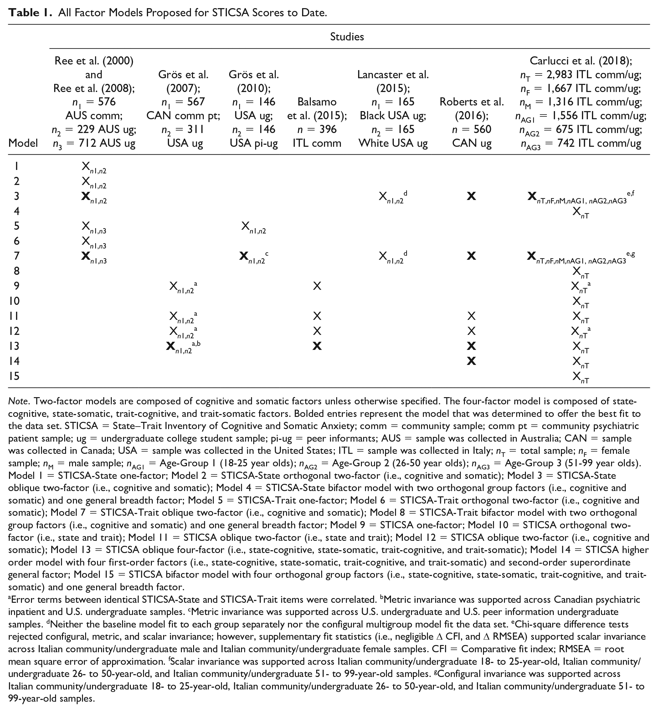
Note. Two-factor models are composed of cognitive and somatic factors unless otherwise specified. The four-factor model is composed of state-cognitive, state-somatic, trait-cognitive, and trait-somatic factors. Bolded entries represent the model that was determined to offer the best fit to the data set. STICSA = State–Trait Inventory of Cognitive and Somatic Anxiety; comm = community sample; comm pt = community psychiatric patient sample; ug = undergraduate college student sample; pi-ug = peer informants; AUS = sample was collected in Australia; CAN = sample was collected in Canada; USA = sample was collected in the United States; ITL = sample was collected in Italy; nT = total sample; nF = female sample; nM = male sample; nAG1 = Age-Group 1 (18-25 year olds); nAG2 = Age-Group 2 (26-50 year olds); nAG3 = Age-Group 3 (51-99 year olds). Model 1 = STICSA-State one-factor; Model 2 = STICSA-State orthogonal two-factor (i.e., cognitive and somatic); Model 3 = STICSA-State oblique two-factor (i.e., cognitive and somatic); Model 4 = STICSA-State bifactor model with two orthogonal group factors (i.e., cognitive and somatic) and one general breadth factor; Model 5 = STICSA-Trait one-factor; Model 6 = STICSA-Trait orthogonal two-factor (i.e., cognitive and somatic); Model 7 = STICSA-Trait oblique two-factor (i.e., cognitive and somatic); Model 8 = STICSA-Trait bifactor model with two orthogonal group factors (i.e., cognitive and somatic) and one general breadth factor; Model 9 = STICSA one-factor; Model 10 = STICSA orthogonal two-factor (i.e., state and trait); Model 11 = STICSA oblique two-factor (i.e., state and trait); Model 12 = STICSA oblique two-factor (i.e., cognitive and somatic); Model 13 = STICSA oblique four-factor (i.e., state-cognitive, state-somatic, trait-cognitive, and trait-somatic); Model 14 = STICSA higher order model with four first-order factors (i.e., state-cognitive, state-somatic, trait-cognitive, and trait-somatic) and second-order superordinate general factor; Model 15 = STICSA bifactor model with four orthogonal group factors (i.e., state-cognitive, state-somatic, trait-cognitive, and trait-somatic) and one general breadth factor.
Error terms between identical STICSA-State and STICSA-Trait items were correlated. bMetric invariance was supported across Canadian psychiatric inpatient and U.S. undergraduate samples. cMetric invariance was supported across U.S. undergraduate and U.S. peer information undergraduate samples. dNeither the baseline model fit to each group separately nor the configural multigroup model fit the data set. eChi-square difference tests rejected configural, metric, and scalar invariance; however, supplementary fit statistics (i.e., negligible ∆ CFI, and ∆ RMSEA) supported scalar invariance across Italian community/undergraduate male and Italian community/undergraduate female samples. CFI = Comparative fit index; RMSEA = root mean square error of approximation. fScalar invariance was supported across Italian community/undergraduate 18- to 25-year-old, Italian community/undergraduate 26- to 50-year-old, and Italian community/undergraduate 51- to 99-year-old samples. gConfigural invariance was supported across Italian community/undergraduate 18- to 25-year-old, Italian community/undergraduate 26- to 50-year-old, and Italian community/undergraduate 51- to 99-year-old samples.
Potential Unmodeled Data Complexity
First, Ree et al. (2008) was the only study that conducted exploratory analyses. Ree et al. reported in a footnote that results of exploratory factor analyses, conducted on the final item pool after CFAs were performed, supported the oblique two-factor model with no items exhibiting cross-loadings ≥.25 on the nontarget factor. This suggests that cross-loadings on nontarget factors up to .24 may have been observed. Yet the oblique two-factor confirmatory model specified by Ree et al. and tested in all studies thereafter adheres to the independent clusters model that constrains nontarget factor loadings to 0.
The independent clusters model assumes that population-level data adhere to a perfect (or approximate) simple structure (Thurstone, 1954), which is appealing in that it creates item subsets assumed to be “pure” indicators of their target factor (i.e., cognitive items are only permitted to load onto the cognitive factor and somatic items are only permitted to load onto the somatic factor). However, results of several studies of commonly administered multifactor rating scales of psychopathology have demonstrated that (a) this assumption may not tenable and (b) constraining nontarget factor loadings to 0 artificially inflates interfactor correlations—even when a CFA model with no cross-loadings fits a data set well (e.g., Herrmann & Pfister, 2013; Howard et al., 2018; Marsh et al., 2010; Morin et al., 2016; Pettersson et al., 2012).
This results in factors that are less distinguishable, which ultimately affects subscore interpretations and the relation between subscores and external variables. For example, Herrmann and Pfister (2013) reported that confirmatory models fit to Revised NEO Personality Inventory (Costa & McCrae, 1992) and 16 Personality Factor Questionnaire–Fifth Edition (Conn & Rieke, 1994) scores from a community sample of adults (n = 620) extracted from the Eugene-Springfield Community Sample (Grucza & Goldberg, 2007) produced overly optimistic estimates of convergent validity and attenuated estimates of divergent validity when both optimally weighted and unit-weighted subscores were related to external criteria. It stands to reason that strict adherence to the independent clusters model in CFA of the STICSA may result in similarly biased relations. Furthermore, permitting STICSA items to cross-load onto nontarget factors could highlight problematic items and/or refine the interpretation of STICSA state–trait cognitive and somatic subscores. Morin et al. (2016) argued that rating scale items are fallible indicators of the constructs they are intended to measure in that they are bound to include at least some degree of relevant association with nontarget factors. The extent to which this occurs on the STICSA, however, remains unknown.
An alternative to traditional CFA is exploratory structural equation modeling (ESEM; Asparouhov & Muthén, 2009). ESEM combines the central features of exploratory factor analysis and CFAs into a single model. The number of factors is determined a priori based on relevant theory (e.g., two for the STICSA representing cognitive and somatic factors) and factor loadings are freely estimated for all items on all factors. CFA models are nested within ESEMs. Therefore, likelihood ratio testing can be conducted to evaluate the tenability of the constraints imposed by the independent clusters model. If the resulting test is statistically significant, then constraining nontarget factor loadings to 0 may not be justifiable.
Overreliance on Unidimensional Modeling
Second, prior research on the STICSA has primarily relied on a unidimensional item-level modeling approach. Bifactor models provide an alternative conceptualization of STICSA scores. In a bifactor model, group factors are derived from the residual common variance remaining after a general breadth factor is extracted from the item correlations (Holzinger & Swineford, 1937). All factors are orthogonal. Hence, item variance is partitioned into its component parts: (a) variance due to the general factor, (b) residual variance due to the group factor after general factor variance is removed, and (c) residual variance due to an amalgam of item specificity and measurement error (i.e., uniqueness). The interitem correlations within a group factor are, therefore, due to multiple dimensions, general factor variance and group factor variance (see Figure 1, Models 4 and 8). Correspondingly, several model-based statistics can be computed from bifactor models in order to determine how “off” item-level multidimensional data would be if it were modeled as unidimensional, how well a set of items represents a latent variable, and which component part explains the most reliable item variance (Rodriguez et al., 2016).
Carlucci et al. (2018) is the only study that applied bifactor models to the STICSA (state and trait forms, separately, and combined). Yet Carlucci et al. applied these models to the Italian version of the scale and they reported that the bifactor model for the STICSA-State and STICSA-Trait, modeled separately, did not converge. Carlucci et al. were successful in estimating a bifactor model for the combined STICSA forms, but they concluded that this model did not fit their data set, and the authors did not provide any model-based statistics as a result.
The Present Study
Different factor models can lead to very different conclusions regarding STICSA score interpretation. Consequently, the primary purpose of the present study was to address these unresolved issues in order to better ascertain what STICSA scores may measure. No prior studies have applied ESEM to the STICSA to our knowledge in order to investigate the tenability of the independent clusters model nor have any prior studies on the STICSA thoroughly explored an item-level multidimensional model. Moreover, prior research on the combined forms of the STICSA evaluating the degree to which STICSA scores differentiate between state–trait cognitive and somatic anxiety has varied with regard to correlating residuals for identical STICSA-State and STICSA-Trait items that load onto the same factor. This makes direct comparison of results across studies impossible. Therefore, a second aim of the present study was to apply Carlucci et al.’s (2018) analytical methods to the combined STICSA forms in order to facilitate comparison of results across studies in which items from both forms are factor analyzed together.
Method
Participants
Participants included 635 students (64.3% female) ranging from 18.0 to 67.9 years old (M = 25.3; SD = 8.1) who were solicited for participation via email from a random sample of 10,000 students at a large, public, 4-year, Hispanic-serving institution of higher education located in the Southwestern United States stratified by sex, race/ethnicity, classification, and college. Response rates <20%, such as those reported in the present study, are not uncommon for large web-based surveys of college students (Sax et al., 2003; Tomsic et al., 2000). Demographic information was obtained from educational records on completion of data collection. Participants included 12.9% freshman, 16.7% sophomores, 22.2% juniors, 27.6% seniors, 2.4% certificate-/non-degree-seeking students, 14.5% master’s degree–seeking students, and 3.8% doctoral students. The racial/ethnic background of participants consisted of 52% Hispanic or Latino/a, 27.4% White, 5.8% Asian, 5% Black or African American, 3.5% two or more races, 3.3% international students, 2.8% unknown or not reported, and 0.2% Native Hawaiian/Other Pacific Islander. Approximately 38.4% of participants were identified as first-generation college students and 34.8% of undergraduate student participants received need-based financial aid (i.e., Pell grant).
Approximately 45.8% of participants obtained a STICSA-Trait total score
Instrument
The STICSA is a 42-item self-report instrument that was developed to measure cognitive and somatic symptoms of state and trait anxiety (Ree et al., 2000; Ree et al., 2008). State and trait forms of the STICSA contain the same 21 items composed of 10 items intended to measure cognitive symptoms (e.g., “I think the worst will happen”) and 11 items intended to measure somatic symptoms (e.g., “I feel dizzy”). Examinees are asked to rate how they feel “right now, at this very moment, even if this is not how you usually feel” on the STICSA-State on a 4-point ordinal scale from not at all (1) to very much so (4), and examinees are asked to rate how they feel “in general” on the STICSA-Trait on a 4-point ordinal scale from almost never at all (1) to almost always (4). Each form of the STICSA yields two subscores: (a) cognitive and (b) somatic. However, four subscores can be obtained by administering both the state and trait forms of the scale together: (a) STICSA-State cognitive, (b) STICSA-State somatic, (c) STICSA-Trait cognitive, and (d) STICSA-Trait somatic.
Cronbach’s (1951)
Procedure
Participants were recruited during the Spring 2018 academic semester via email with a monetary incentive provided by means of a lottery. Students who elected to participate in the study were administered the STICSA-State, STICSA-Trait, and three other measures (a depression inventory, a measure of academic coping strategies, and a measure of academic motivation) in a random order after completing a brief series of questions regarding their use of on-campus mental health resources as part of a larger study on the impact of noncognitive factors on collegiate success. All study measures were administered online using Qualtrics on receipt of university institutional review board approval. Key phrases in the directions for completing the STICSA-State (“ . . . how you feel right now, at this very moment, even if this is not how you usually feel”) and STICSA-Trait (“ . . . how often, in general, the statement is true of you”) were bolded to assist participants in distinguishing between the two forms of the scale. However, a data entry error was committed in which the response options for the STICSA-State (i.e., not at all, a little, moderately, and very much so) were used for both forms. Participants who did not complete both the STICSA-State and STICSA-Trait were excluded from all analyses in the present study. In addition, five participants were excluded from the present study for “flatlining” (no variation in scores; e.g., all 1s) on the depression measure because it contained both positively and negatively worded items (indicating inadequate attention to measures), and 34 participants were excluded from the present study because they participated in the study more than once (duplicate responses).
Analyses
Confirmatory Factor Analysis
CFAs were performed on the item polychoric correlation matrices for the STICSA-State, STICSA-Trait, and combined forms using diagonally weighted least squares with robust standard errors and a mean- and variance-adjusted
The explained common variance (ECV; Sijtsma, 2009; ten Berge & Sočan, 2004) for the general factor, percentage of uncontaminated correlations (PUC; Bonifay et al., 2015; Reise et al., 2013), H index (Hancock & Mueller, 2001), and omega coefficients (Brunner et al., 2012; McDonald, 1999) were computed for all bifactor models. Factor loadings between STICSA items and the general factor produced by a bifactor model would be similar to factor loadings between STICSA items and the general factor produced by an item-level unidimensional model if ECV values are high (ECV > .70).
The PUC is the ratio of the number of correlations between items from different group factors to the total number of correlations in the model. Consequently, high PUC values (>70) would be obtained if the majority of correlations between STICSA items can only be explained by the general factor (i.e., correlations between cognitive anxiety items and somatic anxiety items). It has been demonstrated that the PUC moderates the relationship between the ECV and parameter bias, such that high ECV values lead to parameter bias in models with high PUC values (Bonifay et al., 2015; Reise et al., 2013). Rodriguez et al. (2016) suggested that parameter bias will be negligible when both ECV and PUC are high (>.70).
The H index is an index of construct replicability. It is the ratio of the proportion of explained to unexplained variance in a set of items and it provides an estimate of how well the set of items represents a latent variable (e.g., state–trait cognitive and somatic anxiety). The H index is the correlation between a factor and an optimally weighted composite score. H index values are proportions and factors that are well defined are expected to be replicable across studies (H > .80; Rodriguez et al., 2016).
Finally, omega coefficients were computed to determine (a) the proportion of total variance in the STICSA overall unit-weighted composite score that is due to all sources of common variance (
Relative omega values were also computed to estimate the proportion of common variance in the overall STICSA unit-weighted composite score that is explained by the general breadth factor (dividing
Exploratory Structural Equation Model
ESEM was conducted on the item polychoric correlation matrices for the STICSA-State and STICSA-Trait using WLSMV in Mplus Version 8.3 (Muthén & Muthén, 1998-2017). Two ESEMs were specified in the separate analyses of the state and trait forms of the STICSA. The first ESEM included two factors with an oblique Geomin rotation because prior research has largely supported the oblique two-factor model with moderate to strong positive correlations observed between cognitive and somatic factors (e.g., Grös et al., 2007; Grös et al., 2010; Ree et al., 2008) and the Geomin rotation has been recommended for use in studies in which results from exploratory and confirmatory analyses are compared (Schmitt & Sass, 2011). The second model specified for the separate forms of the STICSA was a bifactor ESEM with two group factors (intended to represent cognitive and somatic latent variables) and an orthogonal Bi-Geomin rotation to determine the degree to which the convergence issues reported in Carlucci et al. (2018) for confirmatory bifactor models could possibly be due to nonnegligible cross-loadings on nontarget factors. Finally, ESEM was also applied to the combined forms of the STICSA to evaluate the tenability of the independent clusters model for confirmatory models that offered the best fit to our data set. The likelihood ratio test was conducted in order to determine the degree to which constraints imposed by the independent clusters model (i.e., zero factor loadings on the nontarget factor) provided a superior fit to the unconstrained ESEMs (Asparouhov & Muthén, 2009).
Model Fit
Conventional criteria to determine adequate model fit were applied to the CFA and ESEM results by inspecting the robust WLSMV
Results
Fit statistics for all factor models are contained in Table 2. Results for the CFA and ESEM conducted on each form of the STICSA, separately, will be reported first followed by results for the CFA and ESEM conducted on the combined STICSA forms.
Fit Statistics for Confirmatory Factor Analyses and Exploratory Structural Equation Modeling of the STICSA-State, STICSA-Trait, and Combined Forms.
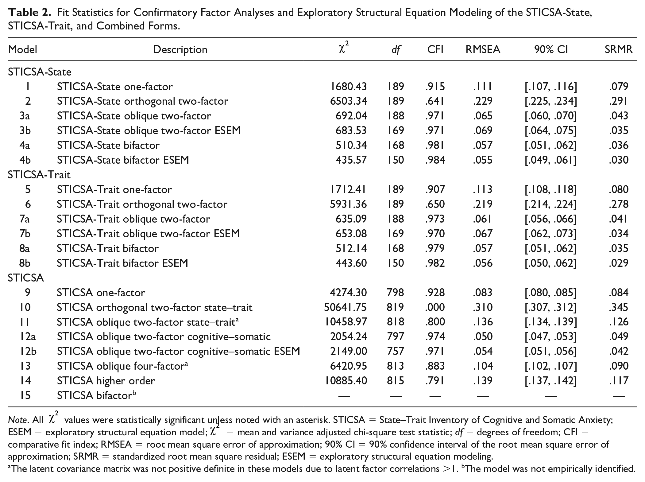
Note. All
The latent covariance matrix was not positive definite in these models due to latent factor correlations >1. bThe model was not empirically identified.
Independent CFA and ESEM on the STICSA-State and STICSA-Trait
CFA of STICSA-State
The one-factor (Model 1) and orthogonal two-factor models (Model 2) did not adequately fit the data set for the STICSA-State. The one-factor model exhibited a CFI of .915, an RMSEA of .111 (95% confidence interval [CI] = [.107, .116]), and an SRMR of .079; and, the orthogonal two-factor model exhibited a CFI of .641, RMSEA of .229 (95% CI = [.225, .234]), and SRMR of .291. However, the oblique two-factor model (Model 3a) provided a good fit to the data set for the STICSA-State as evidenced by a CFI of .971, an RMSEA of .065 (95% CI = [.060, .070]), and an SRMR of .043. The bifactor model (Model 4a) also offered a good fit to the data set for the STICSA-State as evidenced by CFI of .981, an RMSEA of .057 (95% CI = [.051, .062]), and an SRMR of .036. Yet the difference in fit between these two models was negligible, ∆CFI of .01 and ∆RMSEA of −.008.
All standardized factor loadings were statistically significant (p < .001) for the oblique two-factor model. Cognitive and somatic anxiety factors were highly correlated (.76) and all standardized factor loadings were high (
Standardized Factor Loadings for the Confirmatory Oblique Two-Factor Model of the STICSA-State (Model 3a).
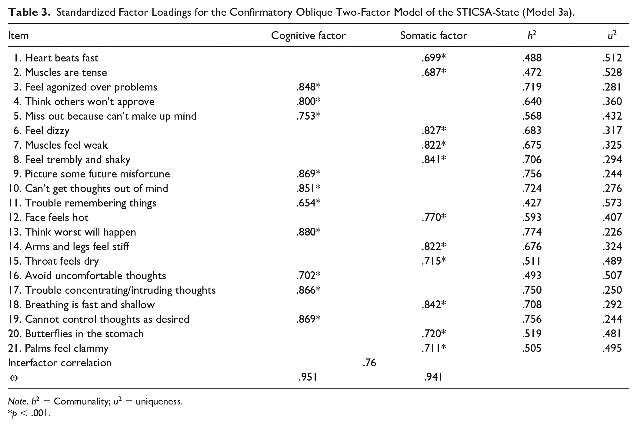
Note. h2 = Communality; u2 = uniqueness.
p < .001.
All standardized factor loadings were statistically significant (p < .001) and salient (
Standardized Factor Loadings for the Confirmatory Bifactor Model of the STICSA-State (Model 4a).

Note. b = Standardized loading of item on factor; Var. = percent variance explained in the item; h2 = communality; u2 = uniqueness;
p < .001.
The general breadth factor was well-defined according to its H index of .964. The somatic group factor was also well-defined according to its H index of .790; albeit, somewhat less well-defined than the general breadth factor. However, the cognitive group factor was not well-defined according to its H index of .385. In addition, 84.5% of the common variance in all 21 STICSA-State items was explained by the general breadth factor. The general breadth factor also contributed the largest proportion of unique, reliable variance in STICSA-State total scores (relative
ESEM of STICSA-State
The oblique two-factor ESEM (Model 3b) offered a good fit to the data set for the STICSA-State as evidenced by CFI of .971, an RMSEA of .069 (95% CI = [.064, .075]), and an SRMR of .035. Moreover, the likelihood ratio test was statistically significant,
Standardized Factor Loadings for the Oblique Two-Factor Exploratory Structural Equation Model of the STICSA-State (Model 3b).

Note. Target factor loadings are in bold. h2 = Communality; u2 = uniqueness.
p < .001.
The bifactor ESEM (Model 4b) also offered a good fit to the data set for the STICSA-State as evidenced by CFI of .984, an RMSEA of .055 (95% CI = [.049, .061]), and an SRMR of .030. However, the ∆CFI of .013 and ∆RMSEA of −.013 between the oblique two-factor ESEM and bifactor ESEM suggest that the difference in fit between these two models is negligible. The likelihood ratio test comparing the confirmatory bifactor model and bifactor ESEM was statistically significant,
Standardized Factor Loadings for the Exploratory Structural Equation Bifactor Model of the STICSA-State (Model 4b).
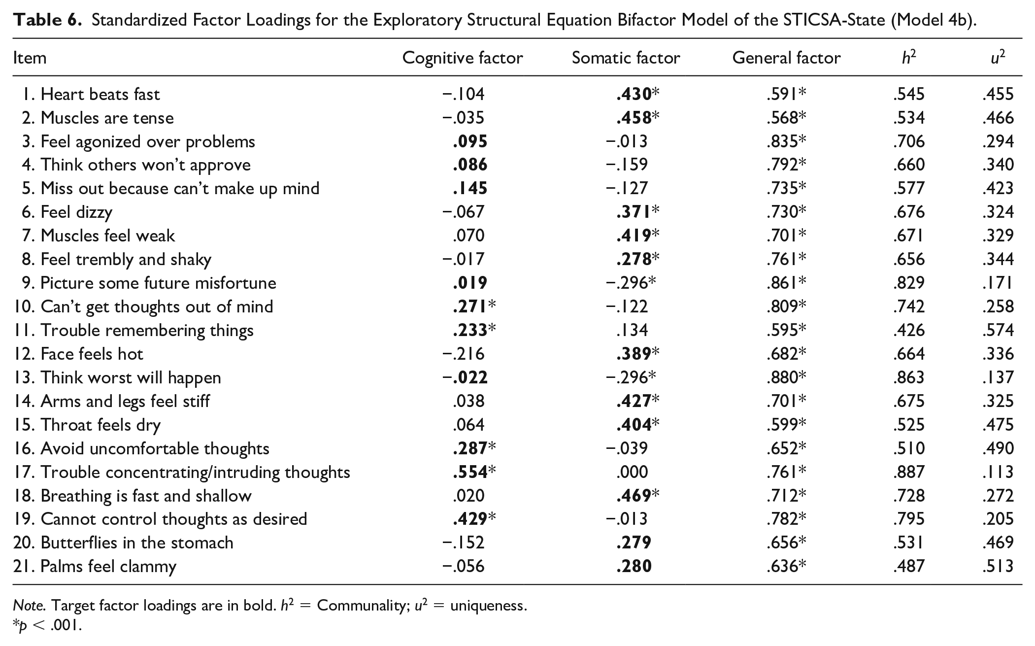
Note. Target factor loadings are in bold. h2 = Communality; u2 = uniqueness.
p < .001.
CFA of STICSA-Trait
The one-factor (Model 5) and orthogonal two-factor models (Model 6) did not adequately fit the data set for the STICSA-Trait. The one-factor model exhibited a CFI of .907, an RMSEA of .113 (95% CI = [.108, .118]), and an SRMR of .080; and, the orthogonal two-factor model exhibited a CFI of .650, RMSEA of .219 (95% CI = [.214, .224]), and SRMR of .278. However, the oblique two-factor model (Model 7a) provided a good fit to the data set for the STICSA-State as evidenced by a CFI of .973, an RMSEA of .061 (95% CI = [.056, .066]), and an SRMR of .041. The bifactor model (Model 8a) also offered a good fit to the data set for the STICSA-State as evidenced by CFI of .979, an RMSEA of .057 (95% CI = [.051, .062]), and an SRMR of .035. Yet the difference in fit between these two models was negligible, ∆CFI of .006 and ∆RMSEA of −−.004.
All standardized factor loadings were statistically significant (p < .001) for the oblique two-factor model for the STICSA-Trait. Cognitive and somatic anxiety factors were highly correlated (.74) and all standardized factor loadings were high (
Standardized Factor Loadings for the Confirmatory Oblique Two-Factor Model of the STICSA-Trait (Model 7a).

Note. h2 = Communality; u2 = uniqueness.
p < .001.
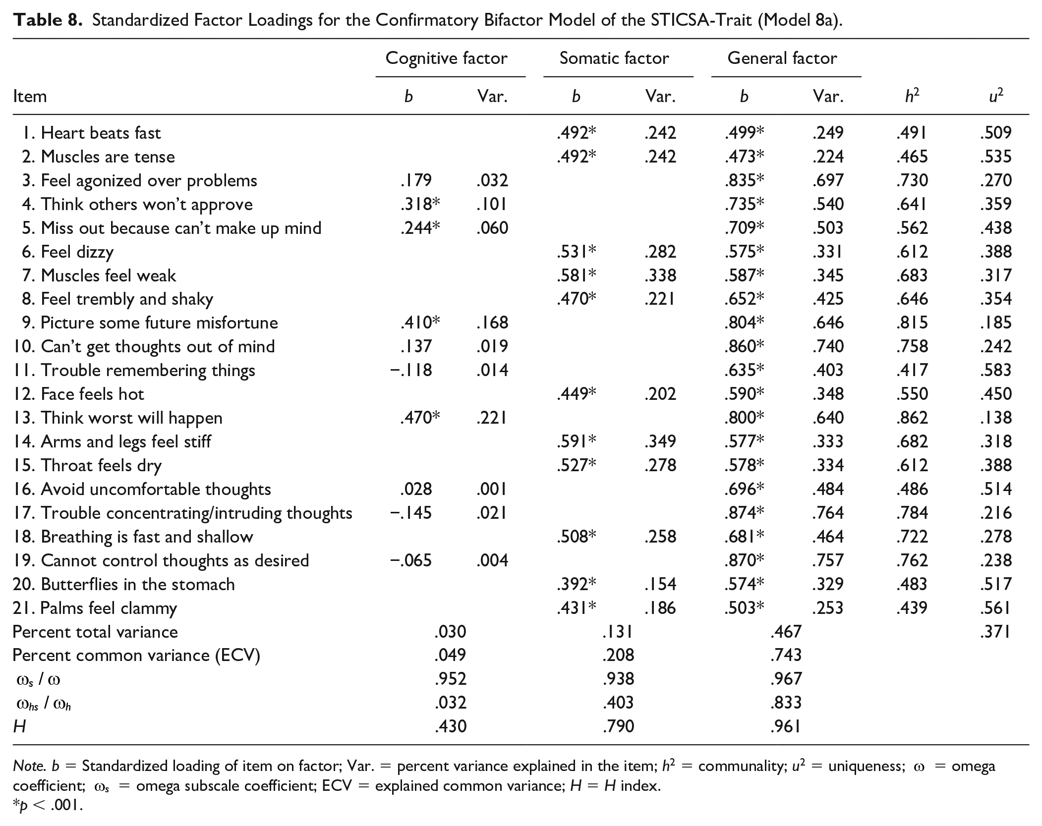
All standardized factor loadings were statistically significant (p < .001) and salient (
Standardized Factor Loadings for the Confirmatory Bifactor Model of the STICSA-Trait (Model 8a).
Note. b = Standardized loading of item on factor; Var. = percent variance explained in the item; h2 = communality; u2 = uniqueness;
p < .001.
The general breadth factor was well defined according to its H index of .961. The somatic group factor was also well-defined according to its H index of .790; though, somewhat less well-defined than the general breadth factor. However, the cognitive group factor was not well defined according to its H index of .430. Additionally, 83.3% of the common variance in all 21 STICSA-Trait items was explained by the general breadth factor. The general breadth factor also contributed the largest proportion of unique, reliable variance in STICSA-Trait total scores (relative
ESEM of STICSA-Trait
The oblique two-factor ESEM (Model 7b) offered a good fit to the data set for the STICSA-Trait as evidenced by CFI of .970, an RMSEA of .067 (95% CI = [.062, .073]), and an SRMR of .034. Moreover, the likelihood ratio test was statistically significant,
Standardized Factor Loadings for the Oblique Two-Factor Exploratory Structural Equation Model of the STICSA-Trait (Model 7b).

Note. Target factor loadings are in bold. h2 = Communality; u2 = uniqueness.
p < .001.
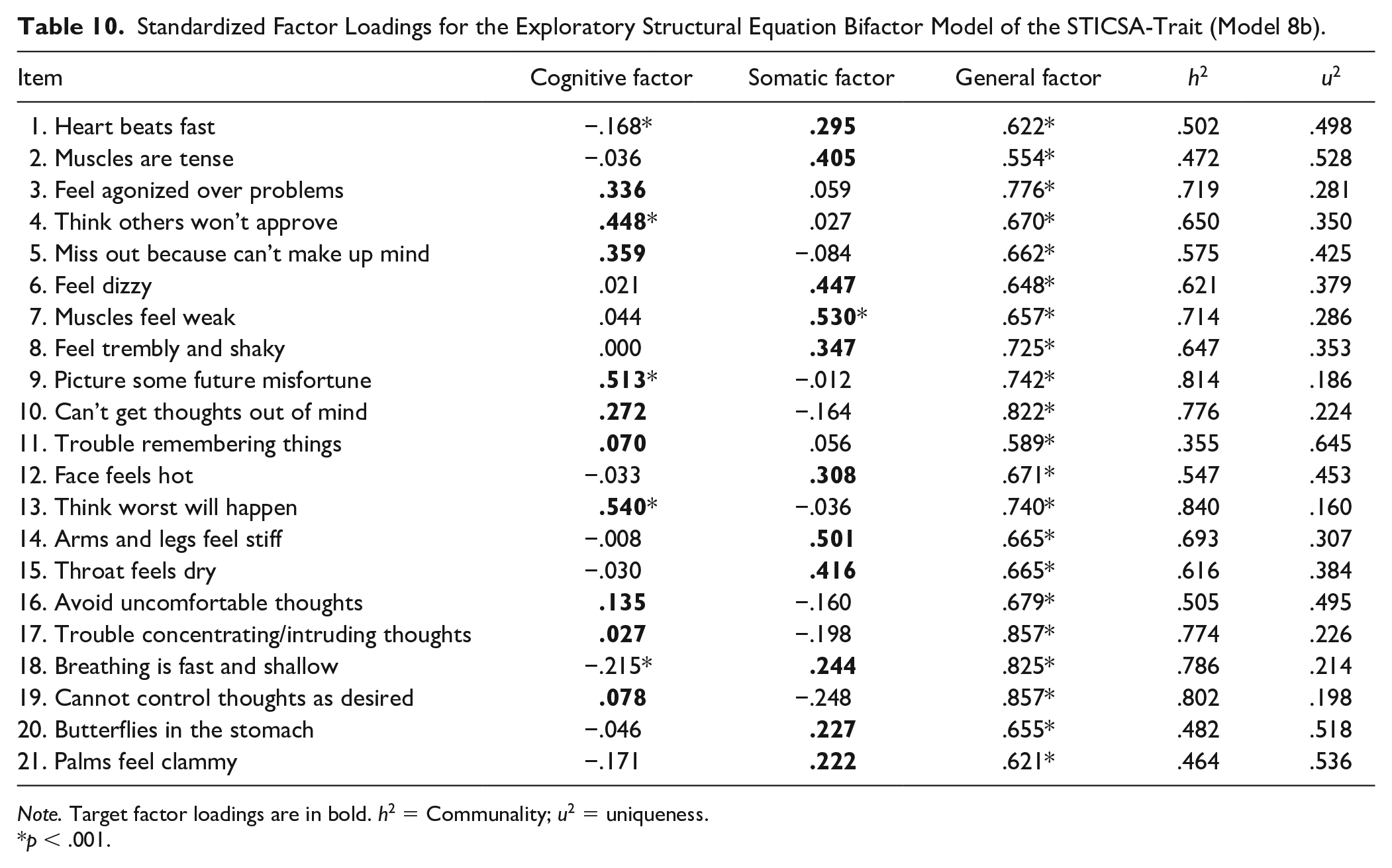
The bifactor ESEM (Model 8b) also offered a good fit to the data set for the STICSA-Trait as evidenced by CFI of .982, an RMSEA of .056 (95% CI = [.050, .062]), and an SRMR of .029. However, the ∆CFI of .012 and ∆RMSEA of −.011 between the oblique two-factor ESEM and bifactor ESEM suggest that the difference in fit between these two models is negligible. The likelihood ratio test comparing the confirmatory bifactor model and bifactor ESEM was statistically significant,
Standardized Factor Loadings for the Exploratory Structural Equation Bifactor Model of the STICSA-Trait (Model 8b).
Note. Target factor loadings are in bold. h2 = Communality; u2 = uniqueness.
p < .001.
Joint CFA and ESEM on the STICSA Combined Forms
CFA of STICSA
The oblique two-factor cognitive–somatic model of the combined STICSA-State and STICSA-Trait forms with correlated residuals for identical STICSA-State and STICSA-Trait items that loaded onto the same factor (Model 12a) was the only confirmatory model that evidenced adequate fit to the data set. The oblique two-factor cognitive–somatic model exhibited a CFI of .974, an RMSEA of .050 (95% CI = [.047, .053]), and an SRMR of .049. In contrast, the latent covariance matrix of the oblique two-factor state–trait (Model 11) and oblique four-factor (Model 13) models were not positive definite due to latent factor correlations >1. The problematic latent factor correlations in the oblique four-factor model included state-cognitive/trait-cognitive and state-somatic/trait-somatic latent variable pairs. Moreover, the bifactor model for the combined STICSA forms was not empirically identified likely due to multicollinearity among identical STICSA-State and STICSA-Trait items that loaded onto the general breadth factor.
All standardized factor loadings were statistically significant (p < .001) for the oblique two-factor cognitive–somatic model for the STICSA. Cognitive and somatic anxiety factors were highly correlated (.75) and all standardized factor loadings were high (
ESEM of STICSA
The oblique two-factor cognitive–somatic ESEM offered a good fit to the data set for the combined STICSA forms (Model 12b) as evidenced by CFI of .971, an RMSEA of .054 (95% CI = [.051, .056]), and an SRMR of .042. Moreover, the likelihood ratio test was statistically significant,
Discussion
The STICSA has become increasingly administered in research on anxiety since its development nearly two decades ago. However, prior studies have relied on a restricted set of confirmatory models to inform STICSA score interpretation that make certain assumptions. Most notably, all factor models fit to STICSA data to date have assumed that items only load onto one factor and that item-level variance is unidimensional (attributed to either variance in latent cognitive or somatic anxiety). However, these assumptions have consequences that may be unintended by the researcher (i.e., inflated/depressed interfactor correlations and biased convergent/divergent relations with external variables; Asparouhov & Muthén, 2009). The resultant purpose of the present study was to investigate the fit of alternative models that relax these assumptions and offer different conceptualizations of STICSA scores (i.e., ESEM and bifactor models) in order to provide a more nuanced picture of what the STICSA may measure.
Results indicated that confirmatory and ESEM versions of both the oblique two-factor (Models 3a-3b and Models 7a-7b) and bifactor models (Models 4a-4b and Models 8a-8b) adequately fit our data set for the separate state and trait forms of the STICSA equally well. Consequently, our findings support the overwhelming majority of research on the STICSA suggesting that each form is well represented by two correlated factors—cognitive and somatic anxiety (Carlucci et al., 2018; Grös et al., 2010; Ree et al., 2008; Roberts et al., 2016). At the same time, our results suggest that these two factors are not equally robust and emphasize the need to consider statistical and conceptual issues in selecting between alternative factor models.
Implications for STICSA Score Interpretation
Results of confirmatory bifactor analyses conducted on each form separately revealed that caution may be warranted when interpreting STICSA state–trait cognitive and somatic subscores (Models 4a and 8a). Unit-weighted cognitive and somatic subscores for our sample on both forms of the STICSA mostly represented variance in a general breadth factor as opposed to variance in latent state–trait cognitive and somatic anxiety. However, the somatic anxiety group factor was much more robust when compared with the cognitive anxiety group factor. For example, the general breadth factor explained 98.5% and 96.6% of the variance in unit-weighted state–trait cognitive subscores, respectively, and 58.2% and 57.0% of the variance in unit-weighted state–trait somatic subscores, respectively. Moreover, results indicated that the somatic group factor approached the threshold of > .80 that has been suggested to indicate a construct that is expected to be highly replicable (Rodriguez et al., 2016) with an H index of .790 for both state and trait forms of the STICSA. However, the cognitive group factor fell well below this threshold with an H index of .385 and .430 for respective STICSA state and trait forms. Within the bifactor model, the general breadth factor is extracted first and the group factors represent remaining common variance in their corresponding item subsets. The general breadth factor for the STICSA-State and STICSA-Trait bifactor models was most strongly indicated by the cognitive items (factor loadings for six items > .80 across state and trait forms), leaving little common variance remaining to be explained by the cognitive group factor. In fact, on the cognitive group factor, factor loadings for only three cognitive items on the STICSA-State and four cognitive items on the STICSA-Trait were statistically significant. In contrast, factor loadings for the general breadth factor for the STICSA-State and STICSA-Trait bifactor models and the somatic group factor converged around .50 with two items on each form loading more strongly onto the somatic group factor than the general breadth factor.
Results also indicated that an optimally weighted STICSA overall composite score derived from a one-factor model would not be equivalent to an optimally weighted STICSA overall composite score derived from the general breadth factor of a bifactor model. Nevertheless, the one-factor model did not adequately fit our data set for either form of the STICSA—a finding that has been consistently reported in other studies as well (Grös et al., 2010; Ree et al., 2000; Ree et al., 2008). Taken altogether, these results suggest that a unit-weighted somatic subscore derived from either form of the STICSA may be a somewhat adequate measure of somatic anxiety and that a unit-weighted cognitive subscore derived from either form of the STICSA may be a relatively pure measure of a general breadth factor. Moreover, our results suggest that an overall composite score of state or trait anxiety derived from the STICSA may be better characterized as mostly a measure of cognitive anxiety.
The ESEM results further complicate interpretation of STICSA subscores by indicating that there is some nonnegligible item overlap across factors (Models 3b, 4b, 7b, and 8b). The oblique two-factor and bifactor ESEMs fit our data set significantly better than the equivalent CFA models for both state and trait forms of the STICSA. Although cross-loadings on nontarget factors were small by conventional standards (<.30; Schmitt & Sass, 2011), this suggests that the assumptions of the independent clusters model (i.e., nontarget factor loadings constrained to 0) may not be tenable for the STICSA and that some STICSA items may measure a mixture of both latent cognitive and somatic anxiety. Among the items with the largest cross-loadings in the present study included “feel agonized over problems” (Item 3), “trouble remembering things” (Item 11), and “feel trembly and shaky” (Item 8). The former two items are intended to measure latent cognitive anxiety but also appear to measure a nonnegligible amount of latent somatic anxiety; whereas, the last item is intended to measure latent somatic anxiety but also appears to measure a nonegligible amount of latent cognitive anxiety. Failing to account for these nonnegligible cross-loadings may produce a misspecified model. For example, an oblique two-factor model that permitted Items 3, 8, and 11 to cross-load onto both cognitive and somatic factors fit significantly better than an oblique two-factor model that adhered to the independent clusters model for both the STICSA-State,
Finally, CFAs conducted on the combined items for the STICSA-State and STICSA-Trait forms indicated that the oblique two-factor cognitive–somatic model fits our data set best (the unconstrained ESEM also fit the data set better than the confirmatory model; Models 12a-12b). As a result, STICSA state–trait cognitive and state–trait somatic factors were not discernible when items from both forms were factor analyzed together. Although Carlucci et al. (2018) reported that this model did not fit their data set, their fit statistics were not substantially below conventional markers of adequate model fit. Consequently, our results are not altogether unexpected. A better test of the degree to which the STICSA adequately distinguishes between state–trait anxiety would require experimental manipulation of state anxiety prior to analyses, which we did not conduct.
Considerations for Final Model Selection
Oblique Two-Factor Model Versus Bifactor Model
Selecting a single suitable model for the STICSA is complicated by our finding that confirmatory and ESEM versions of both the oblique two-factor (Models 3a-3b and Models 7a-7b) and bifactor models (Models 4a-4b and Models 8a-8b) provided an adequate fit to our data set for the separate state and trait forms. It is widely acknowledged that thresholds for model fit indices are arbitrary to the extent that the utility of any given threshold for a particular fit index is a function of many variables, including model complexity, sample size, distributional characteristics of the sample and population data, and so on (e.g., F. Chen et al., 2008; Pitt et al., 2002). Consequently, it has been argued that the degree to which a model aligns with relevant theory and study aims are equally important considerations for final model selection. Moreover, Greene et al. (2019) demonstrated with a series of simulation studies that fit indices tend to favor bifactor models of psychopathology over correlated factor models in the presence of unmodeled correlated residuals (both within and between factors) and cross-loadings in the population when using robust maximum-likelihood or WLSMV with categorical data. The latter finding is particularly noteworthy for the present study, given the superior fit of the ESEMs when compared with the confirmatory factor models for both forms of the STICSA, which suggests that there may be population-level data complexity.
Greene et al. (2019) reported that probifactor bias was present even when model misspecifications were minor (i.e., unmodeled cross-loadings in the population-level model of .10); and, that probifactor bias was most evident in samples of ≤ 1,000 cases with moderate to large cross-loadings (≥.30) in the population-level model that were excluded from confirmatory models fit to the sample data sets. Our study contained 635 cases and results of the oblique two-factor ESEMs indicated that cross-loadings on nontarget factors for the STICSA-State and STICSA-Trait were small to moderate (≤.276). This suggests that differences in fit indices observed between the bifactor and oblique two-factor models in the present study (albeit small) were likely due to the presence of unmodeled complexity in our sample data set (i.e., fit index bias).
One reason for probifactor bias is that the bifactor model has a high fitting propensity (Preacher, 2006; i.e., the average ability of a model to fit data). In particular, the bifactor model is inherently more robust to minor model misspecifications due to unmodeled complexity than correlated factor models. This is primarily due to two factors that affect the fitness propensity of a model. First, the bifactor model has increased parametric complexity (Markon & Krueger, 2004; i.e., more parameters are estimated) when compared with correlated factor models. Larger models tend to fit data sets better than more parsimonious models, though there is a trade-off with generalizability when models overfit a data set (Pitt et al., 2002; Preacher, 2006).
Second, probifactor bias occurs due to the functional form of the parameters estimated in the bifactor model (e.g., Pitt et al., 2002; i.e., the “location” of the estimated parameters). Models that estimate the same number of parameters can differ in functional form and two models with different functional forms, but equivalent free parameters, will exhibit different fitting propensities. Moreover, a model with increased parametric complexity can fit worse than a competing model with fewer free parameters due to differences in functional form (Preacher, 2006). Results of simulation studies indicate that the bifactor model exhibits increased structural complexity (Markon & Krueger, 2004; i.e., increased fitness propensity due to its unique functional form) when compared with correlated factor models or other models nested within it, such as the higher order model (Greene et al., 2019; Murray & Johnson, 2013). The bifactor model is better able to accommodate unmodeled cross-loadings than a correlated factors model by absorbing them as common variance attributed to the general breadth factor. Fit indices that adjust model df to account for differences in parametric complexity, such as those inspected in the current study (i.e., RMSEA and CFI), can be biased because they do not take into account the functional form of the additional parameters in the larger model (e.g., a modeled cross-loading and a factor loading on a general breadth factor are treated the same even though they have different statistical and conceptual implications; Preacher, 2006).
The oblique two-factor model is also nested within the bifactor model. It offers a more parsimonious alternative model for the measurement of the hypothesized cognitive and somatic factors. In certain conditions, the correlated factors and bifactor models are covariance matrix nested (Bentler & Bonett, 1980; i.e., the implied covariance matrix of the correlated factors model can be perfectly reproduced by the bifactor model) and under these conditions the two models are statistically indistinguishable (Bentler & Satorra, 2010). For example, Greene et al. (2019) demonstrated that a bifactor model and a correlated factors model are covariance matrix nested when sample data sets are generated from a population with perfect simple structure and there are no model misspecifications. As a result, fit indices cannot be used to differentiate between these two models. In contrast, Greene et al. reported that the correlated factors and bifactor models were not covariance matrix nested when there was unmodeled complexity in the population-level model, which appears to be the case for the STICSA given our ESEM results.
Independent Clusters Model Versus ESEM
Another choice researchers must make in modeling STICSA scores is between traditional confirmatory approaches to factor analysis that adhere to the independent clusters model and allowing items to load freely onto each hypothesized factor using ESEM. Our ESEM results indicate that the magnitude of freely estimated cross-loadings shifted depending on whether the model was oblique (i.e., oblique two-factor model; Models 3b and 7b) or orthogonal (i.e., bifactor models; Models 4b and 8b). In particular, meaningful cross-loadings in the oblique two-factor ESEM vanished when data were modeled using a bifactor solution. For example, on the STICSA-State, cross-loadings on Items 3, 8, and 11 reduced from .218, .216, and .269 in the oblique two-factor ESEM, respectively, to −.013, −.017, and .134 in the bifactor ESEM. Likewise, on the STICSA-Trait, cross-loadings on Items 3, 8, and 11 reduced from .175, .133, and .276 in the oblique two-factor ESEM, respectively, to .059, .000, and .056 in the bifactor ESEM. Moreover, the correlation between STICSA-State and -Trait cognitive and somatic factors was consistently higher in the CFA models when compared with the interfactor correlation obtained from the ESEMs (.76 vs. .73 and .74 vs. .69, respectively).
These findings are consistent with the literature, which has demonstrated that interfactor correlation bias is inversely related to cross-loading magnitudes (Asparouhov & Muthén, 2009; Schmitt & Sass, 2011). More complex data structures result in lower interfactor correlations. Conversely, cross-loadings are upwardly biased in complex data structures that are modeled using an orthogonal solution (i.e., the relation between factors is reflected in the larger cross-loadings; Schmitt & Sass, 2011). One exception being bifactor models. Rather than reflected in upwardly biased cross-loadings, the relation between factors in complex data structures modeled as a bifactor solution is reflected in the magnitude of loadings on the general breadth factor as demonstrated by the simulation literature (Greene et al., 2019; Murray & Johnson, 2013). This can result in factor collapse, in which factor loadings become near-zero (or negative) and nonsignificant on one or more group factors within a bifactor model. Factor collapse is most evident when interfactor correlations are high (i.e., the population-level model is not a true bifactor solution; Mansolf & Reise, 2016). Interfactor correlations for the STICSA were moderately high in all models (
Limitations
Limitations of the present study include characteristics of our sample. First, participants comprised a convenience sample of college students who volunteered to participate in the study after being solicited for participation over e-mail. Those who volunteered to participate and those who did not may have differed on important demographic characteristics, the presence and/or presentation of anxiety, or on their willingness to self-disclose symptomology on the self-report instruments administered (Hood & Back, 1971). There is also some evidence that research conducted with convenience samples of college students may not generalize to adult community samples (e.g., Hanel & Vione, 2016; Peterson & Merunka, 2014). Second, the bifactor model for the combined forms of the STICSA did not converge when fit to our sample data set. Convergence problems are well documented in bifactor models in general (Greene et al., 2019; Murray & Johnson, 2013) and in prior research on the STICSA (Carlucci et al., 2018), more specifically. Bifactor models are more complex than correlated factors models and this complexity simultaneously increases their fitness propensity and limits their generalizability.
Conclusions
Nevertheless, results of our study indicate that STICSA unit-weighted state–trait cognitive and somatic anxiety composite scores do not purely measure latent cognitive and somatic anxiety as suggested by prior research (Carlucci et al., 2018; Grös et al., 2010; Ree et al., 2008; Roberts et al., 2016). At least three items appear to meaningfully load onto both factors, which complicates STICSA score interpretation. These problems, however, are not unique to the STICSA. The underlying dimensions of any given multidimensional psychological construct are necessarily highly correlated and it is implausible that a human being can write rating scale items in a way that perfectly measures a single dimension. The resulting relations between factors intended to measure each dimension will be merely “moved around” the parameter space, depending on how a researcher wishes to model a sample data set much like water in a water balloon will move to different parts of the balloon depending on how you hold it. The water is always there—it just takes the shape of the balloon that contains it. In a bifactor model, constraining relations between factors to be orthogonal will result in inflated factor loadings on the general breadth factor and (likely) group factor collapse (Mansolf & Reise, 2016). In a correlated factors model, constraining factor loadings on nontarget factors to 0 will result in inflated interfactor correlations (Asparouhov & Muthén, 2009; Marsh et al., 2009; Schmitt & Sass, 2011). In an ESEM, permitting factor loadings to be freely estimated will inflate cross-loadings on nontarget factors and depress interfactor correlations (Asparouhov & Muthén, 2009). Consequently, score interpretation is profoundly impacted by model selection.
Results of our study demonstrated these findings from the literature and underscore the importance of considering context in selecting a factor model. Given that the true population-level model will always be unknown (e.g., Steiger & Schönemann, 1978), researchers must make a choice between competing alternatives that is appropriate for their particular study aims. Bifactor models may be particularly well suited for item development/refinement when the goal is to attain approximate simple structure. However, removing items with large cross-loadings will inevitably reduce interfactor correlations (Schmitt & Sass, 2011) and this may not accurately reflect the true nature of the underlying construct the researcher is attempting to measure. Correlated factors models that adhere to the independent clusters model may be justifiable if the population-level data approximate simple structure. Alternatively, ESEM may be preferred when data are complex. The degree to which items measure more than one factor is an assumption that can be tested by directly comparing confirmatory models that constrain nontarget factors to 0 with ESEM as was conducted in the present study. Failure to do so may lead to inaccurate conclusions regarding convergent/divergent relations with other variables of interest, which can have devastating consequences for theory development. Moreover, advances in ESEM permit analyses of multiple groups, longitudinal data, correlated residuals, and the inclusion of covariates and direct effects that were once only available using confirmatory analytic techniques (Asparouhov & Muthén, 2009). Until researchers demonstrate that psychological attributes can be isolated, it may be advisable to directly model data complexity rather than ignore it.
Supplemental Material
Supplementary_material – Supplemental material for Dimensionality of the State–Trait Inventory of Cognitive and Somatic Anxiety
Supplemental material, Supplementary_material for Dimensionality of the State–Trait Inventory of Cognitive and Somatic Anxiety by Kara M. Styck, Madeline C. Rodriguez and Esther H. Yi in Assessment
Footnotes
Declaration of Conflicting Interests
The author(s) declared no potential conflicts of interest with respect to the research, authorship, and/or publication of this article.
Funding
The author(s) received no financial support for the research, authorship, and/or publication of this article.
Supplemental Material
Supplemental material for this article is available online.
References
Supplementary Material
Please find the following supplemental material available below.
For Open Access articles published under a Creative Commons License, all supplemental material carries the same license as the article it is associated with.
For non-Open Access articles published, all supplemental material carries a non-exclusive license, and permission requests for re-use of supplemental material or any part of supplemental material shall be sent directly to the copyright owner as specified in the copyright notice associated with the article.