Estimating Lifetime and Residual Risk for Individuals Who Remain Sexual Offense Free in the Community: Practical Applications

Abstract

Although individuals with a history of sexual crime are often viewed as a lifelong risk, recent research has drawn attention to consistent declines in recidivism risk for those who remain offense free in the community. Because these declines are predictable, this article demonstrates how evaluators can use the amount of time individuals have remained offense free to (a) extrapolate to lifetime recidivism rates from rates observed for shorter time periods, (b) estimate the risk of sexual recidivism for individuals whose current offense is nonsexual but who have a history of sexual offending, and (c) calculate yearly reductions in risk for individuals who remain offense free in the community. In addition to their practical utility for case-specific decision making, these estimates also provide researchers an objective, empirical method of quantifying the extent to which individuals have desisted from sexual crime.

Keywords

sexual recidivism residual risk extrapolation desistance

A history of sexual crime is a valid risk factor for committing new sexual crimes. For many jurisdictions, this has been sufficient justification for diverse public protection measures that restrict the freedoms of individuals with a history of sexual crime, such as registries, civil commitment, and residence restrictions. Although assessment tools have been developed that measure differences in risk levels between individuals, there has been much less research on assessing changes within individuals. A common interpretation of risk scores based on static (e.g., criminal history) variables is that they assign risk levels that are themselves static, that is, once an individual has been assigned a risk level, that label applies in perpetuity. This is not the case. As documented by the research on desistance, people change, and mostly for the better (Laub & Sampson, 2003; Laws & Ward, 2011; Maruna, 2001).

Although scholars debate the processes and mechanisms of desistance (see Harris, 2014, 2016; Lussier & McCuish, 2016), the more fundamental question of defining desistance remains unresolved. Bushway and colleagues made an important contribution to this debate when they suggested defining desistance statistically (Bushway, Brame, & Paternoster, 2004; Bushway, Piquero, Broidy, Cauffman, & Mazerolle, 2001). Just as actuarial risk tools can be used to identify individuals at high risk to reoffend, they can also be used to identify individuals whose risk for recidivism is below a tolerable threshold (such as the rate of first-time convictions of males in the general population, see, e.g., Blumstein & Nakamura, 2009). Given that true Damascus moments are rare, we can expect, and can statistically model, gradual declines in recidivism risk. Whereas very low risk thresholds are of central concern for those interested in desistance, there are a number of other thresholds of interest for evaluations that inform case management decisions (e.g., bail release, civil commitment, need for sex crime–specific treatment). The lesson of the desistance literature is that the risk of criminal recidivism is not static, even if based on static risk factors—risk predictably declines over time (Hanson, 2018).

For some of these decision thresholds, the concern is with lifetime risk (e.g., desistance, civil commitment). Although an individual with a history of crime may be currently unproblematic, what is the likelihood that this individual will have the intent and the opportunity to offend in the future? Given that most recidivism studies have follow-up times of 10 years or less, decisions based on lifetime rates must rely on some method of extrapolation. Although certain heuristics have been proposed, the field has yet to achieve consensus. For example, Doren (2010) recommended that evaluators estimate the lifetime risk by doubling the 5-year sexual recidivism rate. Wollert and Cramer (2012) criticized the use of a constant multiplier because it poorly replicated the observed rates for different risk levels. Better statistical models are needed.

The purpose of this article is to demonstrate a method of estimating lifetime recidivism rates and for updating risk assessments based on information available after release from the index sexual offense. The method requires only three variables: (a) a numeric estimate of the likelihood of recidivism at time of release; (b) the number of years sex offense free in the community; and (c) whether the individual has a post-index conviction for a nonsexual offense. In this article, we used Static-99R scores to estimate the initial hazard rates. This was partly to be of direct assistance to evaluators who use that instrument, but readers should note that lifetime rates and time free adjustments do not require Static-99R scores; instead, they are intended to apply regardless of the method used to determine the initial risk for recidivism. They can be used with the numeric estimates derived from other risk tools, or even with the overall sexual recidivism base rates observed for a jurisdiction.

The approach in this article uses discrete-time hazard models previously developed by Hanson, Harris, Letourneau, Helmus, and Thornton (2018). Their basic findings were a constant decline in sexual recidivism for each year sexual offense free in the community, and a separate and incremental effect of post-index nonsexual recidivism. Their equations can be used to answer the following three questions: (a) What are the lifetime recidivism rates implied by rates observed for 5- and 10-year follow-up? (b) How to estimate the risk of sexual recidivism for individuals whose current offense is nonsexual but who have a history of sexual offending? (c) How to update risk assessments for individuals who remain offense free in the community?

One criticism of Hanson et al.’s (2018) models is that they may not have sufficiently considered the effect of attaining advance age during follow-up. In the study that leads to a revised age weight for Static-99R (Helmus, Thornton, Hanson, & Babchishin, 2012), there was a strong decline in recidivism risk for individuals who were 60 or older at time of release compared with those who were in their 50s. Consequently, it is possible that there is also a dynamic aging effect associated with attaining certain advanced age thresholds (e.g., turning 60, turning 80). Such thresholds are common in human development, for example, the relationship between age and height is approximately linear only between childhood and late teenage years. Although the direct (linear) effects of aging were included in Hanson et al.’s (2018) models, interactions between time free and specific age thresholds were not examined. Confidence in the new statistical models would be strengthened by explicitly testing the potential effects of critical age thresholds, and if significant, incorporating them into the actuarial scheme.

Being able to generate statistical risk estimates relevant to the three contexts (long-term projections; risk given nonsexual offense subsequent to the index sex offense; time free from any offending) is important, but for such estimates to be used they must be presented in a way that is accessible to their intended audience. The purpose of this article is to develop applications of the new statistical models for these three contexts, translate them into user-friendly procedures that can be applied by evaluators and researchers, and to suggest intelligible ways of explaining the results.

The numbers and tables presented in this article are not fundamentally new. All the values in the tables and figures are implicit in the statistical models presented in Hanson et al. (2018): Specifically, they can be derived from values presented in Model 5 (see Table 4) and Model 6 (see Table 5) from that study. Hanson et al. presented user-friendly figures demonstrating changes in risk over time, but these figures only addressed changes between standardized risk levels. The expected recidivism rates for the various combinations were not presented. Although anyone with the requisite statistical training could use Models 5 and 6 to calculate the recidivism rates presented in the Hanson et al. paper, our experience is that many evaluators would find such calculations daunting. Furthermore, as we worked through the calculations for this paper, we encountered analytic choices that required discussion and decision. Although the outcome of these choices had minimal influence on the overall results, the existence of such choices increased our appreciation of the need for explicit guidance on how these rates should be calculated.

Our general analytic strategy was based on discrete-time survival analysis (Singer & Willett, 2003, Chapter 10). The proportion of individuals with a history of sexual offenses who reoffended after a cumulative time period (e.g., sexual recidivism rates at 5 years) is a function of the proportion who reoffend in each previous time period (i.e., the proportion who reoffend during years 1, 2, 3, 4, and 5). The proportion of at-risk individuals who reoffend in any particular year is called the hazard rate for that year. Because Hanson et al. (2018) found that the change in yearly hazard rates for sexual recidivism was constant (in log odds units), it is possible to estimate from any known (observed) recidivism rate the expected recidivism rates for any other time period.

Readers should note that unless explicitly indicated otherwise we use “reoffending,” “recidivism,” and related terms to refer to observed (detected) offending following sanction for a prior detected offense.

Method

Participants

The 7,225 participants in this study were identical to those used in Hanson et al. (2018). The sample description below is copied or paraphrased from that study. The sample was originally constructed to develop and norm the Static-99R sexual recidivism risk tool (Helmus et al., 2012). All subjects were adult males (18+) with an officially recorded history of sexual crime, a valid Static-99R score, and at least 6 months of follow-up time. The aggregated dataset was constructed from 20 different samples (see Supplemental Table 1), grouped into three broad categories: (a) relatively unbiased samples of routine, complete, or randomly selected sets of cases drawn from a particular jurisdiction (routine/complete samples; k = 8, n = 4,026), (b) individuals referred to specialized sex crime–specific treatment (treatment samples; k = 5, n = 1,899), and (c) individuals preselected to be high risk/high need (k = 5, n = 1,141). The high-risk/high-need samples were expected to be in the top 10% to 15% of the risk distribution and were selected for special measures for individuals deemed high risk to reoffend, such as civil commitment (United States) or detention until warrant expiry (Canada). Treatment samples were those who had been selected from a general population for sex crime–specific treatment. The study included two additional, small samples that did not fit the main categories, namely, a German sample of individuals convicted of sexual murder (n = 86; Hill, Habermann, Klusmann, Berner, & Briken, 2008) and a sample of individuals screened to be low risk (n = 73; Cortoni & Nunes, 2008). These samples were classified as “other.” Individuals were classified according to the study from which they were drawn, and each individual was assigned only one sample type.

For the full sample, the follow-up period ranged from 6 months to 31.5 years (median of 7.2 years, M = 8.2, SD = 5.3 years). Nine samples used charges for a new sexual offense as the recidivism criteria, whereas 11 used convictions. Of the 7,225 individuals, 791 were identified as sexual recidivists. Life-table survival analysis found that the overall sexual recidivism rate was 9.1% at 5 years, 13.3% at 10 years, 16.2% at 15 years, 18.2% at 20 years, and 18.5% at 25 years.

The distributions of individuals from the different sample types varied based on follow-up period. Of the 4,940 individuals followed for 5 years or more, 48.7% were from routine samples. In contrast, only 5.9% of those followed for 15 years or more were from routine samples (64.6% treatment; 25.4% high risk/high need; 4.1% other; total n = 740). Among the 394 individuals followed for more than 20 years, there was only one sexual recidivist: a 63-year-old man who had been in the community for 20.5 years (originally released at age 43). Further description of the sample composition and attrition during follow-up is available in Hanson et al. (2018).

Measures

Static-99R

Static-99R (Helmus, Thornton, et al., 2012) was used as a measure of risk for sexual recidivism at the time of release from the index sexual offense. Static-99R contains 10 items based on commonly available demographic (age, relationship history) and criminal history information (e.g., prior sexual offenses, any unrelated victims, total number of prior sentencing occasions for anything). Static-99R (and its previous version, Static-99) are the sexual recidivism risk assessment tools most commonly used in corrections and forensic mental health (Kelley, Ambroziak, Thornton, & Barahal, 2018; McGrath, Cumming, Burchard, Zeoli, & Ellerby, 2010; Neal & Grisso, 2014). It can be scored with high rater reliability (for a review, see Phenix & Epperson, 2016) and has moderate ability to discriminate recidivists from nonrecidivists (Helmus, Hanson, Thornton, Babchishin, & Harris, 2012).

Static-99R total scores range from −3 to 12 and correspond to the following risk levels: I—very low risk (scores of −3 and −2), II—below-average risk (scores of −1 and 0), III—average risk (scores of 1−3), IVa—above-average risk (scores of 4 and 5), and IVb—well above average risk (scores of 6 and higher; Hanson, Babchishin, Helmus, Thornton, & Phenix, 2017). Static-99R risk levels parallel the standardized risk levels developed for general correctional populations by the Justice Centre of the Council of State Governments (Hanson et al., 2017). These standardized risk levels address the crime-relevant characteristics of individuals in the criminal justice system, the intensity of correctional supervision and rehabilitation programming needed to manage their risk, and their personal strengths and expected prognosis.

In this study, the observed recidivism rates associated with Static-99R scores were used as a plausible range of values from which to estimate the initial annual hazard rates. Specifically, we used the observed 5-year sexual recidivism rates for routine/complete samples. We used both the 5- and 10-year rates for preselected high-risk samples (Hanson, Thornton, Helmus, & Babchishin, 2016; Phenix, Helmus, & Hanson, 2016).

Plan of Analysis

Review of Hanson et al.’s statistical models

Because the estimation procedures used in this study were based on Hanson et al. (2018), an overview of that study is helpful to understanding our analytic approach. Hanson et al. (2018) fit logistic regression equations to discrete-time survival data (Singer & Willett, 1993, 2003; Willet & Singer, 1993). Specifically, follow-up periods were divided into 6-month intervals and the probability of sexual recidivism within these intervals was used as the dependent variable in logistic regression. The person-period dataset contained 105,347 observations (6-month intervals) across 7,225 individuals. Given that the sample size was very large, inclusion or exclusion of predictor variables was based on the Akaike Information Criteria (AIC; Burnham & Anderson, 2004) and the Bayesian Information Criteria (BIC; Raftery, 1995). These are statistical measures of model fit that penalize overfitting. The two models of best fit, used in this study, are presented in Table 1. For those with no convictions up to the time of assessment for post-index nonsexual offending, Hanson et al.’s Model 5 is used. For those with any convictions up to the time of assessment for post-index nonsexual offending Hanson et al.’s Model 6 is used. Although it would be possible to use Model 6 for both groups, we retained separate models because the sample size for Model 5 was substantially larger than the sample size used to derive Model 6 (7,225 vs. 4,078).

Table 1.

Logistic Regression Equations Used to Estimate Annual Hazard Rates With or Without Nonsexual Recidivism.

	Models
	No recidivism (Model 5)	Nonsexual recidivism (Model 6)
No. of individuals (events)	7,225 (791)	4,078 (318)
Parameters
Intercept	−5.002 (.085)	−5.407 (.136)
Time free (years)	−0.130 (.011)	−0.135 (.019)
Static-99R	0.329 (.022)	0.322 (.035)
Sample type (reference category is routine/complete)
Treatment	0.459 (.110)	0.228 (.198)
High risk/high need	0.920 (.136)	1.459 (.193)
Other	−0.705 (.595)	−0.413 (.635)
Interaction: Static-99R by sample type
Treatment × STATIC	−0.081 (.034)	−0.088 (.062)
High risk/high need × STATIC	−0.194 (.053)	−0.137 (.036)
Other × STATIC	0.070 (.146)	0.025 (.162)
Nonsexual recidivism		0.440 (.125)
Overall accuracy (AUC)	0.747	0.755

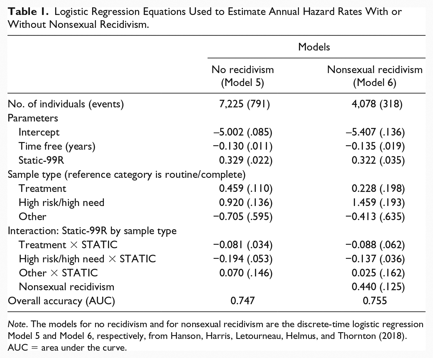
Note. The models for no recidivism and for nonsexual recidivism are the discrete-time logistic regression Model 5 and Model 6, respectively, from Hanson, Harris, Letourneau, Helmus, and Thornton (2018). AUC = area under the curve.

Hanson et al. (2018) found that the logistic distribution adequately fit Models 5 and 6 (nonsignificant Hosmer–Lemeshow goodness-of-fit test). Using Rice and Harris’ (2005) guidelines, the overall predictive accuracy (discrimination) of these models was large, as indicated by area under the curve (AUC) values of .747 (Model 5) and .755 (Model 6). These AUC values can be interpreted as the probability that a recidivist would have a higher predicted probability of recidivism than a nonrecidivist.

In this study, the relevant parameters from Models 5 and 6 are the dynamic effects of (a) time free in the community without sexually reoffending and (b) nonsexual recidivism during follow-up. All the other variables are static, fixed variables that estimate the initial hazard of reoffending sexually at the time of release. In the approach used to estimate the initial hazards, the remaining parameters in Models 5 and 6 should be considered control variables, or covariates, intended to increase the precision of the primary parameter of interest (i.e., the time free effect). The other parameters are not needed for the estimates in this study. Specifically, the values in Table 1 of most direct interest are the time free effect given no new recidivism (b = −.130 [SE = .011]) and, for those with nonsexual recidivism, the combined effect of nonsexual recidivism (b = .440 [SE = .125]) and the independent and incremental effect of time free from sexual offending (b = −.135 [SE = .019]).

Confidence in the size of the time free effect is bolstered by Hanson et al.’s (2018) findings that the time free parameter remained relatively constant regardless of the control variables included: b = −.131 (SE = .011) with no control variables; b = −.123 (SE = .011) with only Static-99R scores; b = −.128 (SE = .011) for Static-99R and sample type (4 types) included; b = −.130 (SE = .011) with Static-99R, sample type, and the interactions between Static-99R and sample type (Model 5); and b = −.135 (SE = .019) for the model that also included nonsexual recidivism (Model 6). Importantly, Hanson et al. (2018) found that the time free effect did not vary based on initial risk levels, as defined by Static-99R scores, or sample type.

The values provided in Table 1 are in logits, or log odds units, of the yearly hazard rates: ln(hazard rate/[1 – hazard rate]). This means that when the time free effect is b = −.130, there is a reduction of .130 log odds units of sexually recidivating for each consecutive year in the community without reoffending, or a reduction of e –.1³⁰ = .878095 in the odds of recidivism per year. Nonsexual criminal recidivism increases the odds of recidivism in any particular year by 1.55 (e^.440 = 1.55).

Discrete-time survival analysis

The discrete-time approach (see, e.g., Singer & Willett, 2003, Chapter 10) estimates recidivism rates based on the proportion of individuals who reoffend during a discrete time period divided by the number of individuals available to reoffend during that time period. This ratio is called a hazard (h_t) and can assume values from zero (no recidivists in that time period) to 1.0 (all available individuals reoffend). The subscript t indicates that the hazard rate is a variable that can take different values for different years (i.e., h₃ refers to the hazard rate in year 3, and h_t is the general form indicating the hazard rate for t different years).

The proportion of individuals surviving any single time interval is one minus the hazard rate for that interval (s_t = 1 – h_t). Conversely, the recidivism rate is one minus the proportion surviving (i.e., the hazard rate). The cumulative proportion surviving ( S _T) is the product of the proportion who has not previously reoffended (i.e., the proportion still at risk [p_{at risk}]) and the proportion not reoffending during that specific time interval:

S_{T} = p_{a t r i s k} \times [1 - h_{t}] o r S_{T} = p_{a t r i s k} \times s_{t} .

With a consistent decline in hazard rates over time (known from previous research), yearly hazard rates can be estimated from any observed recidivism rate for any length of time (e.g., yearly rates can be estimated from 2-year, 5-year, 7.6-year, or any other fixed follow-up period).

Once the expected hazard rates are estimated for each year, the cumulative survival is estimated using the hazard rates projected into all future years. Given that the hazard of reoffending is negligible after 20 years, follow-up ended at that time, that is, the hazard rate after 20 years sexual offense free was set to zero.

As stated previously, the cumulative survival rate, S _T, is the product of the survival rates (1 – h_t) of each year at risk:

S_{T} = \prod_{year = 1}^{t} (1 - h_{t}) .

(1)

Given the constant annual reduction in the logit of the hazard rate, it is useful to express the hazards in Formula 1 in logit units:

S_{T} = \prod_{year = 1}^{t} (1 - (\frac{1}{1 + e^{- (logit (h_{t}))}})) .

(2)

Formula 2 is identical to Formula 1, except that the hazard rate is first transformed into logit units, ln(h/[1 – h]), then retransformed back into a proportion, p = 1/(1 + e^–logit(h)). This transformation makes it easy to increment the logit of the yearly hazard rate by a constant (e.g., b = −.130):

S_{T} = \prod_{y = 1}^{t} (1 - (\frac{1}{1 + e^{- (logit (h_{1}) + (y - 1) b)}})) .

(3)

For example, if b = −.130 and the observed 3-year sexual recidivism rate is 10% (90% survival), Formula 3 would be written as follows:

. 90 = (1 - (\frac{1}{1 + e^{- (logit (h_{1}))}})) (1 - (\frac{1}{1 + e^{- (logit (h_{1}) - . 130)}})) (1 - (\frac{1}{1 + e^{- (logit (h_{1}) - . 260)}})) .

This equation has a single positive solution for h₁ (the hazard rate for the first year), although the algebra is complicated. Consequently, rather than solve each equation for h₁, the value of h₁ was estimated to four significant figures through iteration using an Excel spreadsheet. For example, the initial 1-year hazard rate for a Static-99R score of 3 was just more than 2% (.02073) for routine/complete samples (see Supplemental Table 2).

Extrapolation from 5- or 10-year recidivism rates to 20-year rates

Three sets of observed recidivism rates were used to estimate initial hazard rates (i.e., hazard rates at time of release) associated with Static-99R scores: the observed 5-year sexual recidivism rates for routine/complete samples, the 5-year rates for preselected high-risk samples, and the 10-year rates for the preselected high-risk samples (Hanson et al., 2016; Phenix et al., 2016). The resulting estimates for h₁ are presented in Supplemental Table 2.

Once the hazard rates at time of release were estimated, the hazard rates for subsequent years were calculated by subtracting .130 from the logit of the hazard rate for the previous year: logit(h_t _{+ 1}) = logit(h_t) – .130. The logit was then transformed back into proportions, and Formula 1 was used to calculate the cumulative survival rates for follow-up times up to 20 years offense free.

Assessing the risk for sexual recidivism following a nonsexual offense

The same initial hazard rates (see Supplemental Table 2) were used when estimating risk for individuals with a history of sexual crime but who reoffend nonsexually after release from their index sex offense. Here “nonsexual” reoffenses refer to convictions for new offenses, not to technical violations. For each full year that they were sexual offense free, .135 was subtracted from the logit of the hazard of the previous year. This applied to each year in the community, except the year in which the individual received his first nonsexual conviction. During the year of nonsexual recidivism, .440 was added to the logit of the hazard for the previous year. This was added only once and remained for the rest of the follow-up period. No credit was given for being sexual offense free during the year of first nonsexual conviction. In all subsequent follow-up years, however, the time free reduction was applied.

Revising initial risk assessment years based on time offense free in the community

At time of release, individuals face risk of sexually recidivating presented in 20 intervals: the cumulative hazards for year 1 to year 20. The hazard rate after 20 years was set to zero. When an individual has remained offense free for x years, his residual risk was calculated using the hazard rates for his subsequent years at risk (i.e., year_{x + 1} to year₂₀). The initial start values (hazard rates at release) were those provided in Supplemental Table 2. The time free effect for individuals who did not have any post-release nonsexual convictions was set at –.130 of the logit of the hazard of the previous year. The logits of the hazard values were then transformed back into proportions and used to estimate residual risk using Formula 1.

Estimating errors of recidivism estimates

Three approaches were used to examine the margin of error of calculated estimates. The first approach compared the initial hazard values inferred from the observed recidivism rates for the preselected high-risk groups at 5 years and for the same group at 10 years. If the relative decline is as constant as we propose, then similar estimates should be produced regardless of the follow-up period used to infer the initial estimates.

The second approach examined how much the results changed when the calculations used the full range of values included in the 95% confidence intervals of the time free parameter (±1.96 × SE). Specifically, estimates were computed based on the values of −0.15156 and −0.10844 (calculated as −0.130 ± [1.96 × 0.011]). A limitation of this approach is that the size of the standard error is primarily influenced by the total sample size, which was very large (105,347 observations).

The third approach examined how much the results changed based on the different values of the time free parameter in the different logistic models (see Tables 4 and 5 from Hanson et al., 2018). In the plausible models, these values ranged from –.123 (SE = .011) to –.135 (SE = .019).

Results

As a preliminary step, we examined whether there was any evidence of incremental effects of turning 60, 70, or 80 in the community. None were found. In the full dataset of 7,225 individuals, the average age at release was 39.9 years (SD = 12.2) with a range from 18 to 84. The average age at the end of the follow-up (survival end date, i.e., the earlier of recidivism date or end of follow-up) was 47.2 (SD = 12.9), with a range of 19 to 103 years. There were 1,174 individuals who were 60 or older, 399 who were 70 or older, and 84 who were 80 or older at some point during the follow-up period. There were no recidivists in the dynamic 80+ age group. The oldest recidivist was 76 years old and had been in the community for 3.5 years.

In the logistic model that included time free, Static-99R total scores, sample type, and the interaction of sample type and Static-99R as covariates (Hanson et al., 2018, Model 5; 105,347 observations, 791 sexual recidivists), neither turning 60, turning 70, or turning 80 improved the prediction of sexual recidivism. Nor did any of these age thresholds statistically interact with time free (all AIC and BIC changes were positive, i.e., in the direction of worsening model fit). The incremental effects of turning 60, turning 70, and turning 80 were also tested in a simpler model that only included time free and Static-99R scores (not sample type) as covariates, and again they did not improve model fit (all AIC and BIC changes were positive). In other words, although individuals in these older dynamic age groups demonstrated low sexual recidivism rates, these low levels of risk were expected given their Static-99R scores at time of release (including age at release) and their years offense free in the community.

Extrapolations to 20-year recidivism rates

Extrapolation to 20-year sexual recidivism rates involved estimating the annual hazard at time of release based on observed recidivism rates and then using these initial hazards (see Supplemental Table 2) to project forward based on the consistent decline over the observed 20-year follow-up period. The results of these projections are shown for routine/complete samples based on 5-year observed rates (see Table 2) and for preselected high-risk/high-need samples based on 5-year observed rates (see Table 3) and on 10-year observed rates (see Table 4). These risk estimates are relevant to evaluators who are assessing long-term risk subsequent to release from the index sex offense. The assessment is normally made prior to this release and relates to risk at the point of release.

Table 2.

Estimated Sexual Recidivism Rates (Percentages) for Follow-Up Periods Ranging From 6 to 20 Years for Routine/Complete Samples Based on Observed 5-Year Recidivism Rates.

Follow-up year	Initial risk (based on Static-99R scores)
	Level I		Level II		Level III			Level IVa		Level IVb
	−3	−2	−1	0	1	2	3	4	5	6	7	8	9	10
5	0.9	1.3	1.9	2.8	3.9	5.6	7.9	11.0	15.2	20.5	27.2	35.1	43.8	53.0
6	1.0	1.5	2.2	3.2	4.4	6.3	8.9	12.4	17.1	22.9	30.2	38.8	48.0	57.6
7	1.1	1.6	2.4	3.5	4.9	7.0	9.8	13.6	18.6	25.0	32.8	41.9	51.5	61.3
8	1.2	1.8	2.6	3.8	5.2	7.5	10.5	14.6	20.0	26.7	35.0	44.4	54.4	64.3
9	1.3	1.9	2.7	4.0	5.6	8.0	11.2	15.5	21.2	28.3	36.9	46.6	56.8	66.7
10	1.4	2.0	2.9	4.2	5.9	8.4	11.8	16.3	22.2	29.6	38.5	48.5	58.8	68.8
11	1.4	2.1	3.0	4.4	6.1	8.8	12.3	17.0	23.1	30.7	39.9	50.0	60.4	70.4
12	1.5	2.1	3.1	4.6	6.4	9.1	12.7	17.6	23.9	31.7	41.0	51.4	61.9	71.9
13	1.5	2.2	3.2	4.7	6.6	9.4	13.1	18.1	24.6	32.5	42.1	52.5	63.1	73.0
14	1.6	2.3	3.3	4.9	6.7	9.6	13.5	18.5	25.2	33.3	42.9	53.5	64.1	74.0
15	1.6	2.3	3.4	5.0	6.9	9.8	13.8	18.9	25.7	33.9	43.7	54.4	65.0	74.9
16	1.6	2.4	3.5	5.1	7.0	10.0	14.0	19.3	26.2	34.5	44.4	55.1	65.8	75.6
17	1.7	2.4	3.5	5.2	7.1	10.2	14.2	19.6	26.5	35.0	44.9	55.7	66.4	76.2
18	1.7	2.4	3.6	5.2	7.2	10.3	14.4	19.8	26.9	35.4	45.4	56.3	67.0	76.8
19	1.7	2.5	3.6	5.3	7.3	10.5	14.6	20.1	27.2	35.7	45.9	56.8	67.5	77.2
20	1.7	2.5	3.7	5.4	7.4	10.6	14.8	20.3	27.5	36.1	46.3	57.2	67.9	77.6

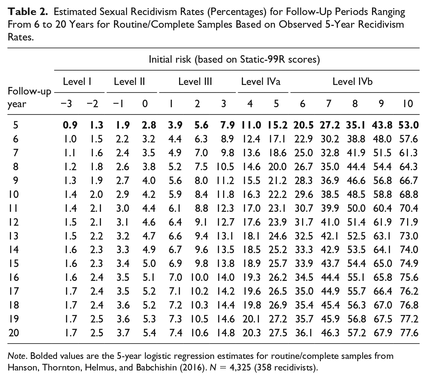
Note. Bolded values are the 5-year logistic regression estimates for routine/complete samples from Hanson, Thornton, Helmus, and Babchishin (2016). N = 4,325 (358 recidivists).

Table 3.

Estimated Sexual Recidivism Rates (Percentages) for Follow-Up Periods Ranging From 6 to 20 Years for High-Risk/High-Need Samples Based on Observed 5-Year Recidivism Rates.

Follow-up year	Initial risk (based on Static-99R scores)
	Level I		Level II		Level III			Level IVa		Level IVb
	−3	−2	−1	0	1	2	3	4	5	6	7	8	9	10
5			5.6	7.2	9.0	11.3	14.0	17.3	21.2	25.7	30.7	36.3	42.2	48.4
6			6.3	8.1	10.1	12.7	15.7	19.4	23.7	28.6	34.0	40.1	46.3	52.9
7			7.0	8.9	11.1	13.9	17.2	21.2	25.8	31.1	36.9	43.2	49.8	56.5
8			7.5	9.6	12.0	15.0	18.5	22.7	27.6	33.2	39.2	45.8	52.6	59.4
9			8.0	10.2	12.7	15.9	19.6	24.0	29.2	35.0	41.3	48.1	54.9	61.9
10			8.4	10.8	13.4	16.7	20.6	25.2	30.5	36.5	43.0	49.9	56.9	63.9
11			8.8	11.2	14.0	17.4	21.4	26.2	31.7	37.8	44.4	51.5	58.6	65.6
12			9.1	11.6	14.5	18.0	22.1	27.0	32.7	39.0	45.7	52.9	60.0	67.0
13			9.4	12.0	14.9	18.5	22.8	27.8	33.6	40.0	46.8	54.0	61.2	68.2
14			9.6	12.3	15.3	19.0	23.3	28.4	34.3	40.8	47.7	55.0	62.2	69.2
15			9.8	12.6	15.6	19.4	23.8	29.0	35.0	41.6	48.5	55.9	63.1	70.1
16			10.0	12.8	15.9	19.8	24.2	29.5	35.5	42.2	49.2	56.6	63.9	70.9
17			10.2	13.0	16.2	20.1	24.6	29.9	36.0	42.8	49.8	57.3	64.5	71.5
18			10.3	13.2	16.4	20.3	24.9	30.3	36.5	43.2	50.4	57.8	65.1	72.1
19			10.5	13.4	16.6	20.6	25.2	30.6	36.8	43.7	50.8	58.3	65.6	72.5
20			10.6	13.5	16.7	20.8	25.4	30.9	37.2	44.0	51.2	58.8	66.0	73.0

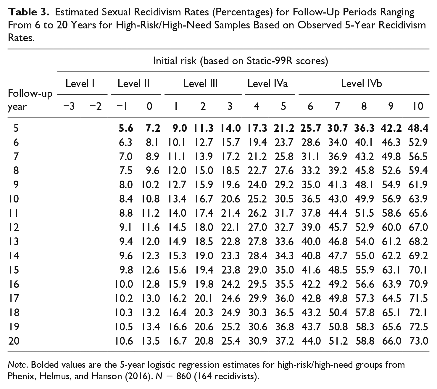
Note. Bolded values are the 5-year logistic regression estimates for high-risk/high-need groups from Phenix, Helmus, and Hanson (2016). N = 860 (164 recidivists).

Table 4.

Estimated Sexual Recidivism Rates (Percentages) for Follow-Up Periods of 5 and 11 to 20 Years for High-Risk/High-Need Samples Based on Observed 10-Year Recidivism Rates.

Follow-up year	Initial risk (based on Static-99R scores)
	Level I		Level II		Level III			Level IVa		Level IVb
	−3	−2	−1	0	1	2	3	4	5	6	7	8
5			7.1	8.7	10.7	13.0	15.7	18.8	22.4	26.3	30.6	35.1
10			10.6	13.0	15.8	19.1	22.9	27.3	32.1	37.3	42.8	48.5
11			11.1	13.6	16.5	19.9	23.8	28.4	33.3	38.6	44.3	50.1
12			11.5	14.0	17.0	20.6	24.6	29.3	34.3	39.8	45.5	51.4
13			11.8	14.5	17.5	21.2	25.3	30.1	35.2	40.8	46.6	52.6
14			12.1	14.8	18.0	21.7	25.9	30.8	36.0	41.7	47.5	53.6
15			12.4	15.2	18.4	22.1	26.4	31.4	36.7	42.4	48.4	54.4
16			12.6	15.4	18.7	22.5	26.9	31.9	37.3	43.1	49.1	55.1
17			12.8	15.7	19.0	22.9	27.3	32.4	37.8	43.6	49.7	55.8
18			13.0	15.9	19.3	23.2	27.7	32.8	38.3	44.1	50.2	56.3
19			13.2	16.1	19.5	23.4	28.0	33.1	38.7	44.6	50.6	56.8
20			13.3	16.3	19.7	23.7	28.2	33.4	39.0	44.9	51.0	57.2

Note. Bolded values are the 10-year logistic regression estimates for high-risk/high-need groups from Phenix, Helmus, and Hanson (2016). N = 350 (98 recidivists).

To use these tables, evaluators need to know the individual’s Static-99R score and whether the individual has sufficient density of external risk factors (i.e., risk factors not measured by the Static-99R risk tool) to justify placement in the high-risk/high-need reference group (i.e., whether or not to use Table 2 for routine/complete samples; for a discussion on selecting reference groups for Static-99R norms, see Hanson et al., 2016). Of the two tables for the high-risk/high-need samples (see Tables 3 and 4), our preference is Table 4 because it requires less extrapolation than Table 3. On the contrary, some evaluators may prefer Table 3 to Table 4 because the 5-year sexual recidivism norms are based on more samples with a larger total N than the 10-year norms. Consistency between estimates in Table 3 and those in Table 4 provides one check on the potential error associated with the extrapolation method.

As shown in Table 2, for the average risk group (Level III), the 10-year rates were approximately 1.5 times the 5-year rates, and the 20-year rates were approximately double the 5-year rates. For a Static-99R score of 2 (the median value), the observed 5-year sexual recidivism rate was 5.6%, the cumulative 10-year rate was 8.4%, and the cumulative 20-year rate was 10.6%. The same pattern was observed for the very low risk group (Level I) and the below-average risk group (Level II). As the initial risk levels increased, however, the 20-year rates were less than double the 5-year rates. For example, for a Static-99R score of 8, the observed 5-year rate was 35.1% and the cumulative 20-year rate was 57.2% (not 70.2%).

The maximum lifetime recidivism risk for individuals classified as Level I (very low risk) was 2.5% (Static-99R scores of −3 and −2), which would translate to an applied decision threshold of less than three out of 100 individuals. Rates this low were only observed in routine/complete samples; no individuals from the high-risk samples met this threshold at time of release. Conversely, if decisions involve a high risk threshold of lifetime recidivism rates of 35% or more, then this would correspond to Static-99R scores of 6+ (well above average) in routine/complete samples, or 5+ in preselected high-risk/high-need samples.

Risk Assessment Given a Post-Index Nonsexual Offense

Tables 5 and 6 present the 20-year sexual recidivism rates for individuals with a history of sexual crime, but who were convicted of a nonsexual offense subsequent to their release from their index sex offense. For this analysis, the risk for sexual recidivism was again assumed to be zero after 20 years sexual offense free in the community. For the high-risk/high-need samples, the projections were based on the estimated initial hazard rates estimated from the observed 10-year rates. These are the recidivism estimates relevant to evaluators wishing to assess the risk presented by individuals with a history of sexual offending who have come to attention because they have committed a nonsexual offense after release from their index sex offense. However, it can also be used for any individual who has had a new nonsexual conviction following release from an index sexual offense, for example, individuals with a sexual offending history who have been several years on community supervision for a nonsexual offense. In this case, the follow-up year would be years at liberty in the community since the index sexual offense, subtracting time served from calendar time.

Table 5.

Projected Residual Risk (Sexual Recidivism Rates as Percentages) From Time of Release Up to 20 Years Sex Offense Free in the Community for Routine/Complete Samples by Time of First Nonsexual Recidivism.

Follow-up year	Initial risk (based on Static-99R scores)
	Level I		Level II		Level III			Level IVa		Level IVb
	−3	−2	−1	0	1	2	3	4	5	6	7	8	9	10
<1	2.6	3.8	5.5	8.0	11.0	15.5	21.4	28.9	38.2	48.8	60.4	71.6	81.3	88.9
1	2.3	3.3	4.7	6.9	9.6	13.6	18.8	25.5	34.1	44.1	55.3	66.6	76.8	85.3
2	2.0	2.8	4.1	6.0	8.3	11.8	16.5	22.5	30.3	39.5	50.2	61.3	71.9	81.2
3	1.7	2.4	3.5	5.2	7.2	10.3	14.4	19.7	26.8	35.2	45.2	56.1	66.7	76.5
4	1.5	2.1	3.1	4.5	6.2	8.9	12.5	17.2	23.5	31.2	40.5	50.8	61.3	71.4
5	1.2	1.8	2.6	3.9	5.4	7.7	10.8	15.0	20.6	27.5	36.0	45.7	55.9	66.0
6	1.1	1.5	2.2	3.3	4.6	6.6	9.3	13.0	17.9	24.0	31.7	40.7	50.4	60.4
7	0.9	1.3	1.9	2.8	3.9	5.7	8.0	11.1	15.4	20.9	27.8	36.0	45.1	54.8
8	0.8	1.1	1.6	2.4	3.3	4.8	6.8	9.5	13.3	18.0	24.1	31.5	39.9	49.1
9	0.6	0.9	1.4	2.0	2.8	4.1	5.8	8.1	11.3	15.4	20.8	27.4	35.0	43.5
10	0.5	0.8	1.2	1.7	2.4	3.4	4.9	6.8	9.6	13.1	17.7	23.5	30.3	38.0
11	0.5	0.7	1.0	1.4	2.0	2.8	4.1	5.7	8.0	11.0	15.0	20.0	25.9	32.8
12	0.4	0.5	0.8	1.2	1.6	2.3	3.3	4.7	6.6	9.1	12.5	16.7	21.9	27.9
13	0.3	0.4	0.6	0.9	1.3	1.9	2.7	3.8	5.4	7.4	10.2	13.8	18.1	23.3
14	0.2	0.3	0.5	0.7	1.0	1.5	2.2	3.0	4.3	6.0	8.2	11.1	14.7	19.0
15	0.2	0.3	0.4	0.6	0.8	1.2	1.7	2.4	3.3	4.6	6.4	8.7	11.6	15.1
16	0.1	0.2	0.3	0.4	0.6	0.9	1.2	1.8	2.5	3.5	4.8	6.5	8.7	11.4
17	0.1	0.1	0.2	0.3	0.4	0.6	0.9	1.2	1.7	2.4	3.4	4.6	6.2	8.1
18	0.1	0.1	0.1	0.2	0.3	0.4	0.5	0.8	1.1	1.5	2.1	2.9	3.9	5.1
19	<0.1	<0.1	0.1	0.1	0.1	0.2	0.3	0.4	0.5	0.7	1.0	1.4	1.8	2.4
20	0.0	0.0	0.0	0.0	0.0	0.0	0.0	0.0	0.0	0.0	0.0	0.0	0.0	0.0

Note. Recidivism rate projections based on 5-year logistic regression estimates from Hanson, Thornton, Helmus, and Babchishin (2016). Underlined values mark the transition out of Level IVb (above 35%) and into Level I (less than 3%).

Table 6.

Projected Residual Risk (Sexual Recidivism Rates as Percentages) From Time of Release Up to 20 Years Sex Offense Free in the Community for High-Risk/High-Need Samples by Time of First Nonsexual Recidivism.

Follow-up year	Initial risk (based on Static-99R scores)
	Level I		Level II		Level III			Level IVa		Level IVb
	−3	−2	−1	0	1	2	3	4	5	6	7	8	9	10
<1			19.3	23.4	28.1	33.4	39.2	45.6	52.3	59.0	65.5	71.7
1			17.0	20.6	24.8	29.6	35.0	41.0	47.3	53.8	60.3	66.6
2			14.8	18.1	21.9	26.2	31.1	36.7	42.6	48.8	55.1	61.4
3			12.9	15.8	19.2	23.1	27.5	32.6	38.1	43.9	50.0	56.1
4			11.2	13.8	16.7	20.2	24.2	28.8	33.8	39.3	45.0	50.8
5			9.7	11.9	14.5	17.6	21.2	25.3	29.9	34.8	40.2	45.7
6			8.4	10.3	12.6	15.3	18.4	22.1	26.2	30.7	35.6	40.8
7			7.2	8.8	10.8	13.2	15.9	19.2	22.8	26.9	31.3	36.0
8			6.1	7.5	9.2	11.3	13.7	16.5	19.7	23.3	27.3	31.6
9			5.2	6.4	7.9	9.6	11.7	14.1	16.9	20.1	23.6	27.4
10			4.4	5.4	6.6	8.1	9.9	12.0	14.4	17.1	20.2	23.5
11			3.6	4.5	5.5	6.8	8.3	10.0	12.1	14.4	17.1	20.0
12			3.0	3.7	4.6	5.6	6.8	8.3	10.0	12.0	14.2	16.7
13			2.4	3.0	3.7	4.5	5.6	6.8	8.2	9.8	11.7	13.8
14			1.9	2.4	2.9	3.6	4.4	5.4	6.6	7.9	9.4	11.1
15			1.5	1.9	2.3	2.8	3.4	4.2	5.1	6.2	7.4	8.7
16			1.1	1.4	1.7	2.1	2.6	3.2	3.8	4.6	5.5	6.5
17			0.8	1.0	1.2	1.5	1.8	2.2	2.7	3.2	3.9	4.6
18			0.5	0.6	0.7	0.9	1.1	1.4	1.7	2.0	2.4	2.9
19			0.2	0.3	0.3	0.4	0.5	0.6	0.8	1.0	1.1	1.4
20			0.0	0.0	0.0	0.0	0.0	0.0	0.0	0.0	0.0	0.0

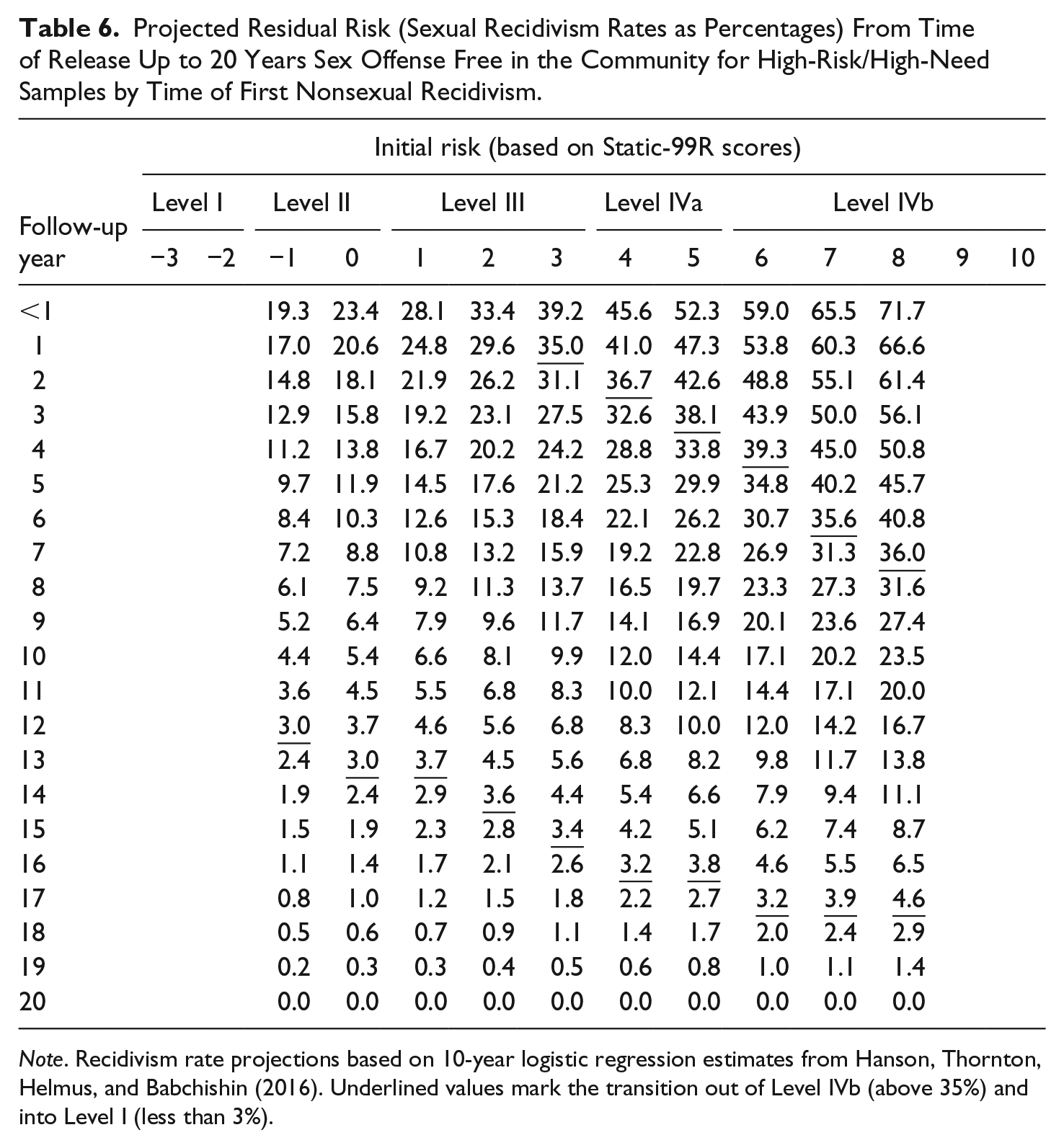
Note. Recidivism rate projections based on 10-year logistic regression estimates from Hanson, Thornton, Helmus, and Babchishin (2016). Underlined values mark the transition out of Level IVb (above 35%) and into Level I (less than 3%).

To use these tables, evaluators need to know the individual’s Static-99R score, the number of years offense free in the community prior to the first nonsexual offense conviction, and whether the individual has sufficient density of external risk factors to justify placement in the high-risk/high-need reference group (i.e., whether to use Table 5 or 6). The numbers in the tables are the percentage of individuals expected to commit another sexual offense were they to be followed up to 20 years. For example, the expected 20-year sexual recidivism rates for those in the middle of the risk distribution (Static-99R score of 2) is 15.5% should they be convicted of a nonsexual offense during the first year at liberty. This rate declines to 7.7% if their first nonsexual conviction was in year 5.

It is interesting to note that, even with nonsexual offending, all individuals with a history of sexual offenses will still drop below a low risk threshold of 3% should they remain sexual offense free in the community long enough. As shown in Table 5, for the very low risk group (Level I), individuals in routine/complete samples are below this threshold after 1 year. For the below-average group (Level II), it is between 5 and 7 years; for the average risk group (Level III), it is between 9 and 13 years; and for the above-average groups in routine/complete samples (Level IVa and Level IVb), it is between 14 and 19 years.

Conversely, for high-risk/high-need samples, 20-year sexual recidivism rates of 35% or higher would be expected for individuals with Static-99R scores as low as 3 if they were convicted for a new nonsexual offense soon after release. A score of 3 is typically considered average, with projected lifetime recidivism rates of 14.8% (routine/complete samples; see Table 2); however, if the individuals had a score of 3, were classified as high risk/high need, and reoffend with a nonsexual offense within the first year at liberty, their expected 20-year sexual recidivism rate would now be 39.2% (39 out of 100). Individuals placed in Risk Level IVb (well above average; Static-99R scores of 6+) would still have lifetime sexual recidivism rates above the 35% threshold if they refrained from sexual offending but reoffend nonsexually within the first 5 years in the community.

Residual Risk for Individuals With No New Offending

Tables 7 and 8 present the residual risk for individuals who have remained free of both sexual and nonsexual convictions while in the community. Table 7 presents the rates for routine/complete samples; Table 8 presents the rates for preselected high-risk/high-need samples using the observed 10-year rates. The first rows of Tables 7 and 8 are the same as the last rows of Tables 2 and 4, respectively. In other words, the first rows of Tables 7 and 8 are the 20-year projected recidivism risk from the time of release. The longer the individuals remain offense free, the lower their risk of subsequently committing a new sexual offense. These are the recidivism estimates that are relevant to evaluators who wish to assess the risk now presented by someone who has been in the community for some time without reoffending after release from their index sex offense.

Table 7.

Projected Residual Risk (Sexual Recidivism Rates as Percentages) From Time of Release Up to 20 Years Offense Free in the Community for Routine/Complete Samples.

Follow-up year	Initial risk (based on Static-99R scores)
	Level I		Level II		Level III			Level IVa		Level IVb
	−3	−2	−1	0	1	2	3	4	5	6	7	8	9	10
At release	1.7	2.5	3.7	5.4	7.4	10.6	14.8	20.3	27.5	36.1	46.3	57.2	67.9	77.6
1	1.5	2.2	3.2	4.7	6.5	9.3	13.0	17.9	24.3	32.2	41.8	52.3	62.9	72.9
2	1.3	1.9	2.8	4.1	5.6	8.1	11.3	15.7	21.5	28.7	37.5	47.4	57.8	68.0
3	1.1	1.6	2.4	3.5	4.9	7.0	9.9	13.7	18.9	25.4	33.4	42.7	52.7	62.8
4	1.0	1.4	2.1	3.0	4.2	6.1	8.6	12.0	16.6	22.3	29.7	38.3	47.7	57.6
5	0.8	1.2	1.8	2.6	3.7	5.3	7.5	10.4	14.4	19.6	26.2	34.0	42.9	52.3
6	0.7	1.0	1.5	2.3	3.2	4.5	6.6	9.0	12.5	17.1	22.9	30.1	38.2	47.2
7	0.6	0.9	1.3	1.9	2.7	3.9	5.5	7.8	10.8	14.8	20.0	26.4	33.8	42.1
8	0.5	0.8	1.1	1.6	2.3	3.3	4.8	6.6	9.3	12.7	17.3	23.0	29.6	37.3
9	0.4	0.6	0.9	1.4	2.0	2.8	4.0	5.6	7.9	10.9	14.8	19.8	25.7	32.6
10	0.4	0.5	0.8	1.2	1.6	2.4	3.4	4.8	6.7	9.2	12.6	16.9	22.1	28.3
11	0.3	0.5	0.7	1.0	1.4	2.0	2.8	4.0	5.6	7.8	10.6	14.3	18.8	24.2
12	0.3	0.4	0.5	0.8	1.1	1.6	2.3	3.3	4.6	6.4	8.9	12.0	15.8	20.4
13	0.2	0.3	0.4	0.7	0.9	1.3	1.9	2.7	3.8	5.3	7.2	9.8	13.0	17.0
14	0.2	0.2	0.4	0.5	0.7	1.1	1.5	2.1	3.0	4.2	5.8	7.9	10.5	13.8
15	0.1	0.2	0.3	0.4	0.6	0.8	1.2	1.7	2.4	3.3	4.5	6.2	8.3	10.9
16	0.1	0.1	0.2	0.3	0.4	0.6	0.9	1.2	1.8	2.5	3.4	4.7	6.2	8.2
17	0.1	0.1	0.1	0.2	0.3	0.4	0.6	0.9	1.2	1.7	2.4	3.3	4.4	5.8
18	<0.1	0.1	0.1	0.1	0.2	0.2	0.4	0.5	0.8	1.1	1.5	2.1	2.8	3.7
19	<0.1	<0.1	<0.1	0.1	0.1	0.1	0.2	0.3	0.4	0.5	0.7	1.0	1.3	1.7
20	0.0	0.0	0.0	0.0	0.0	0.0	0.0	0.0	0.0	0.0	0.0	0.0	0.0	0.0

Table 8.

Projected Residual Risk (Recidivism Rates as Percentages) From Time of Release Up to 20 Years Offense Free in the Community for High-Risk/High-Need Samples.

Follow-up year	Initial risk (based on Static-99R scores)
	Level I		Level II		Level III			Level IVa		Level IVb
	−3	−2	−1	0	1	2	3	4	5	6	7	8
At release			13.3	16.3	19.7	23.7	28.2	33.4	39.0	44.9	51.0	57.2
1			11.7	14.3	17.3	20.9	25.1	29.8	35.0	40.5	46.3	52.3
2			10.2	12.5	15.2	18.4	22.1	26.5	31.2	36.3	41.8	47.5
3			8.9	10.9	13.3	16.2	19.5	23.4	27.6	32.4	37.4	42.8
4			7.7	9.5	11.6	14.1	17.1	20.5	24.4	28.7	33.3	38.3
5			6.7	8.2	10.1	12.3	14.9	18.0	21.4	25.3	29.5	34.1
6			5.8	7.1	8.7	10.7	12.9	15.6	18.7	22.1	25.9	30.1
7			5.0	6.1	7.5	9.2	11.2	13.5	16.2	19.3	22.7	26.4
8			4.2	5.2	6.4	7.9	9.6	11.6	14.0	16.7	19.7	23.0
9			3.6	4.4	5.5	6.7	8.2	9.9	12.0	14.3	16.9	19.8
10			3.0	3.7	4.6	5.7	6.9	8.4	10.2	12.2	14.4	17.0
11			2.5	3.1	3.9	4.7	5.8	7.1	8.5	10.2	12.2	14.3
12			2.1	2.6	3.2	3.9	4.8	5.9	7.1	8.5	10.1	12.0
13			1.7	2.1	2.6	3.2	3.9	4.8	5.8	7.0	8.3	9.8
14			1.3	1.7	2.1	2.5	3.1	3.8	4.6	5.6	6.7	7.9
15			1.0	1.3	1.6	2.0	2.4	3.0	3.6	4.4	5.2	6.2
16			0.8	1.0	1.2	1.5	1.8	2.2	2.7	3.3	3.9	4.7
17			0.5	0.7	0.8	1.0	1.3	1.6	1.9	2.3	2.8	3.3
18			0.3	0.4	0.5	0.6	0.8	1.0	1.2	1.4	1.7	2.1
19			0.2	0.2	0.2	0.3	0.4	0.5	0.6	0.7	0.8	1.0
20			0.0	0.0	0.0	0.0	0.0	0.0	0.0	0.0	0.0	0.0

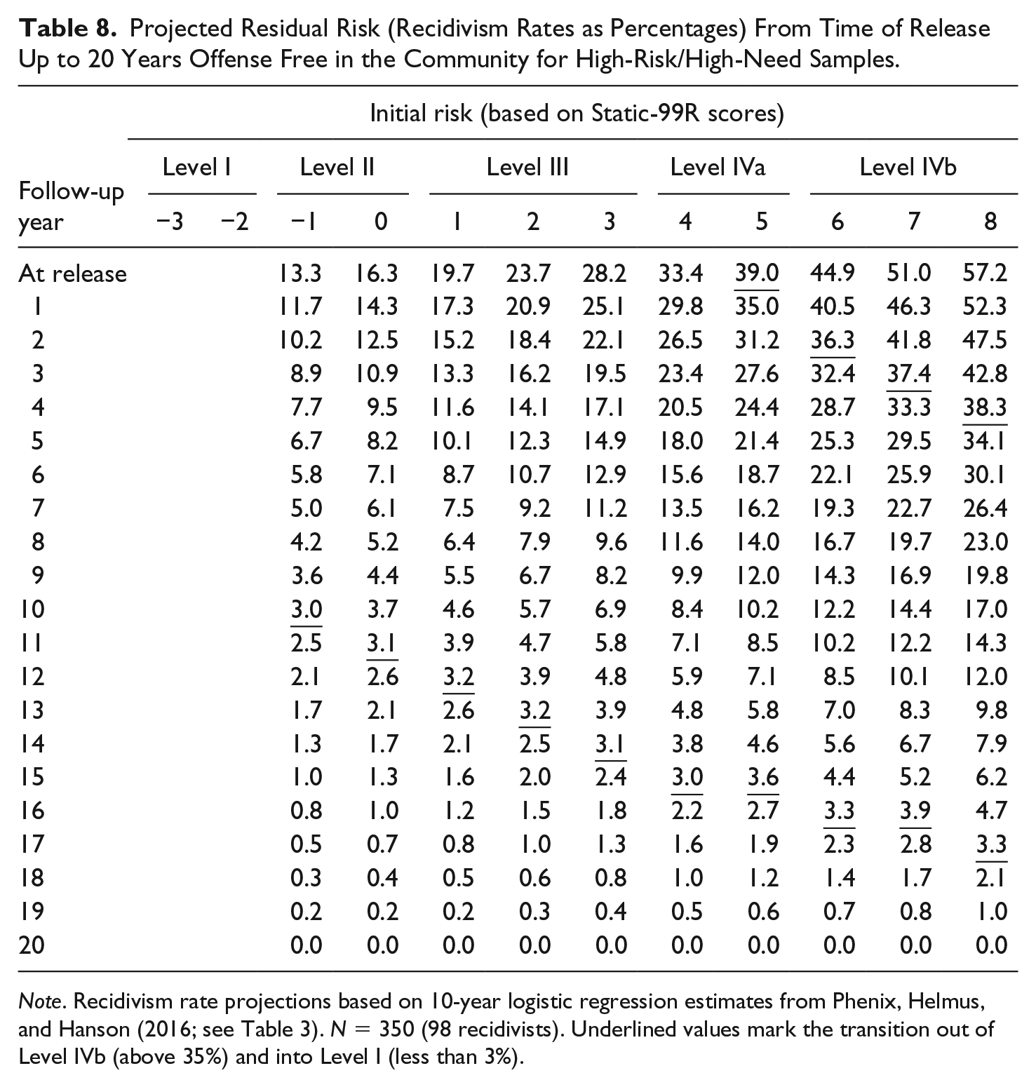
Note. Recidivism rate projections based on 10-year logistic regression estimates from Phenix, Helmus, and Hanson (2016; see Table 3). N = 350 (98 recidivists). Underlined values mark the transition out of Level IVb (above 35%) and into Level I (less than 3%).

For individuals whose initial risk was above a high risk threshold of 35% or more, the vast majority (Static-99R scores of 8 or lower) drop below this threshold if they remain in the community offense free for 5 years, and all individuals drop below this high risk threshold by 9 years. If they stay offense free long enough, all individuals will eventually drop below the very low risk threshold (<3%), regardless of their initial risk score.

Error estimates

Comparison of Tables 3 and 4 provides an indication of the degree of error. Table 3 projects forward to 10 years based on the observed 5-year rates; Table 4 projects backward to 5-year rates using the observed 10-year rates. Although the samples are not identical (not all individuals followed for 5 years were also followed for 10 years), both are from the same population (high risk/high need). As readers can see, the differences between the observed rates and the projections were typically within 2 percentage points. The 10-year forward projections from the observed 5-year rates were slightly lower than the observed 10-year rates, although the differences were small (median difference of −1.5% [range of −1.2 to +1.7]). Similarly, the backward projections to 5 years from the observed 10-year rates were slightly higher than the observed 5-year rates (median difference of 2.2% [range of −2.4 to 1.4]). There was also high concordance between the 20-year projections based on the observed 5-year rates and the 20-year projections based on the 10-year rates (median difference of 2.6%, range of −1.5% to 2.9%).

The second approach to estimating error examined the range of values included in the 95% confidence intervals of the time free parameter (b ± 1.96 × SE). Specifically, estimates were computed based on the b values of –.15156 and –.10844 (–.130 ± [1.96 × 0.011]). These values are presented in Figure 1 for the Static-99R scores of 0, 2, 4, and 6. These Static-99R scores were selected because they are the most populated values for Risk Levels II, III, IVa, and IVb. The results for Risk Level I were not presented because they were very similar to those for Risk Level II.

Figure 1.

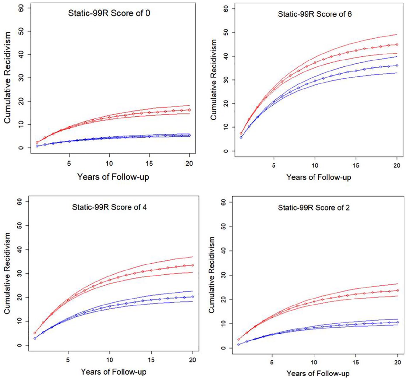
Cumulative recidivism rates over 20 years of follow-up with 95% confidence intervals for selected Static-99R risk levels.

As depicted in Figure 1, the confidence intervals were within a couple of percentage points when the absolute recidivism rates were small (<15%) and the follow-up time was less than 10 years. The widest confidence intervals (approximately ± 5 percentage points) were observed when the follow-up was greater than 15 years and the absolute values were more than 30%. For example, the estimated 20-year cumulative sexual recidivism rate for the group defined by Static-99R scores of 6 in high-risk/high-need samples was 44.9% (see Table 4), and the 95% confidence interval ranged from 41.2% to 49.2%.

The third approach to estimating error examined how much results change based on the range of values for the time free parameter in the different logistic models from –.123 to –.135 (see Tables 4 and 5 from Hanson et al., 2018). These values are well within the range defined by the 95% confidence interval for the time free parameters (−0.15156, −0.10844); consequently, using the observed variation in the parameters across models results in a smaller range of error estimates than using the range defined by the 95% confidence intervals for the main analysis. For example, given a score of 6 in routine/complete samples (estimated 20-year rate of 36.1%), the confidence interval approach indicates a range 7 percentage points wide (32.9%, 39.8%) and the variation in the parameters approach suggests a range 2 percentage points wide (35.3%, 37.2%).

In summary, given known initial hazard rates, the 20-year projections would be expected to have error rates of between ±1 percentage points and ±5 percentage points, with larger error rates associated with larger estimated recidivism rates.

Discussion

The aim of this article was to demonstrate how the constant time free effect observed in Hanson et al. (2018) provides solutions to three challenges currently faced by evaluators interested in empirical estimates of sexual recidivism risk: (a) lifetime recidivism rates, (b) risk when the index offense is not a sexual offense, and (c) declines in risk for individuals who remain offense free in the community. The approaches used in this article should also be of interest to desistance researchers interested in an objective approach to quantifying the likelihood that individuals have permanently desisted from sexual offending.

The statistical model included only three variables: (a) years sexual offense free while in the community, (b) whether the individual was convicted of a post-index nonsexual offense, and (c) a numeric estimate of the likelihood of recidivism during the first year after release from the index sexual offense. In this study, we used Static-99R scores to estimate the initial likelihood; however, similar patterns would be expected regardless of the method used to estimate the initial hazards. Declining marginal hazards is one of the most robust findings in all of criminology (Kurlychek, Bushway, & Brame, 2012).

Although the Static-99R has moderate accuracy (discrimination; Helmus, Hanson, et al., 2012), it does not measure all relevant risk factors. Some of these external factors could be available to evaluators at time of release, such as response to institutional treatment (Olver et al., 2018), or the density of psychologically meaningful risk factors (e.g., Thornton & Knight, 2015). Other variables can only be known after release, such as the quality of their psychological and community adjustment (McGrath, Lasher, & Cumming, 2012) and the receipt of effective community supervision (Duwe & Freske, 2012; Seto, Sandler, & Freeman, 2017). Consequently, evaluators need to consider the empirical risk estimates presented in this article as part of an overall evaluation of risk.

As demonstrated in Figure 1, the choice of the initial hazard values has much greater consequences for the final estimates than the estimated error in the time free effects. Previous research has observed a wide range of recidivism rates associated with specific Static-99R scores (Helmus, Hanson et al., 2012); the test developers responded to this (unwanted) variation by providing two sets of recidivism rate tables: one for routine/complete samples and another for samples preselected as high risk (Phenix et al., 2016). For all but the highest Static-99R scores, the differences between these reference groups can be substantial. For example, given a Static-99R of 4, the routine/complete samples had estimated 20-year rates of 20% (see Table 2), whereas the rate for the high-risk/high-need groups was 33% (see Table 4). In other words, the choice of the initial hazard rate could result in a 13 percentage point difference, whereas using the extremes of the confidence intervals for the time free estimates would only result in a 4% to 6% difference.

This study provided partial support for Doren’s (2010) assertion that lifetime sexual recidivism rates are approximately twice the rates observed after 5 years. Doren’s heuristic reasonably represented the results for lower and average risk groups. For higher risk groups, however, this heuristic overestimates risk compared with the discrete-time survival method used in this study. Furthermore, using a simple risk ratio or multiplier could potentially result in impossible values (e.g., risk estimates greater than 100%). In contrast, the discrete-time method provides more precise estimates than Doren’s (2010) approach and can be used across the full range of risk levels and follow-up times.

Applied Uses

Estimation of long-term sexual recidivism rates

Most definitions of desistance are concerned with cessation of offending, not just temporary pauses in a life otherwise full of crime. Consequently, the concept of (very low) lifetime rates is central to desistance theory and research. The tables in this study could provide useful guidance to researchers interested in estimating the likelihood that individuals who claim to have stopped sexual offending will never reappear in the criminal justice system for this type of offense. For example, in Harris’ (2016) desistance study, she included as “desisting” individuals who made no cognitive changes, and were described as lonely, pessimistic, and defeatist. Given that most of these individuals had been released for less than 4 years (and some as recently as a few months), critics could argue that these individuals remain at significant risk for sexual recidivism. A much stronger test of the patterns of desistance would begin by sorting the participants based on estimates of their lifetime recidivism rates.

Lifetime recidivism rates are also important in certain legal contexts. For most cases, these long-term risk estimates are made before the individual has been released (e.g., Sexually Violent Persons (SVP) cases in the United States). It is important to note that these long-term risk estimates are generated at the time the individual is being evaluated and do not include the time free effect because the individuals have not yet been released into the community. The exception to this is when an individual’s SVP commitment occurred following reincarceration for a nonsexual offense conviction, or because his community supervision was revoked. In those cases, any time free effect, increased risk due to nonsexual offending, and custody time should be incorporated into the risk estimates. Given that we can only assess risk with the information we have at the time of assessment, risk should be considered dynamic. An individual’s recidivism risk should be expected to change over time in response to life circumstances. Repeated assessments after individuals have been released to the community would provide information about decreasing sexual recidivism risk (or, conversely, their continued risk due to nonsexual offending).

When the governing offense is not the index sex offense

Evaluators may struggle when completing sexual risk assessments for individuals with a history of sex offending but whose most recent offense was not a sex offense. How does one incorporate factors that may have occurred since the individual was released from the index sex offense? Previously, evaluators would use their professional judgment to combine time free effects with actuarial risk scores, which could lead to diverse decisions of unknown validity. With this study, evaluators have a fully actuarial method to account for nonsexual offending and periods of custody post-release.

Risk assessments for those in the community who have not reoffended

Individuals with a history of sex offenses often undergo risk assessments in the community to determine their treatment and risk management needs. The current statistical model provides important information to aid recommendations in such evaluations. This information provides explicit guidance relevant to risk management and decisions regarding when interventions should increase treatment and/or supervision resources due to nonsexual offending, or reduce interventions due to successful survival in the community without reoffending. It can also provide information for how resources might best be allocated over the next 5 to 10 years. By considering time free effects, community-based agencies responsible for helping individuals transition into the community from jail or prison can project individuals’ sexual recidivism risks more precisely to determine how long clients need to be on their caseload.

In the United States and elsewhere, individuals may be evaluated to determine the need for inclusion on a registry. The purported purpose of such registries is to contribute to public safety through educating local authority personnel and/or the public about individuals in their community (e.g., https://www.justice.gov/criminal-ceos/sex-offender-registration-and-notification-act-sorna). Those included on a registry will then normally be subject to more intensive monitoring. Inclusion on such registries, however, has far-reaching consequences for the identified individuals (e.g., residence and work restrictions; Laws, 2016; Levenson, Grady, & Leibowitz, 2016). The degree to which registries are able to achieve their stated purpose will depend, in part, on the extent to which those registered actually pose a risk for sexual offending. As a class, adults convicted of sex offenses do pose a risk for future sex offending that is several times the risk posed by adults released following sentences for nonsexual offenses (e.g., Alper & Durose, 2019). Not all members of this class, however, pose the same risk, and the potential effectiveness of registries will be diluted by the inclusion of individuals who have desisted from sexual offending. In some U.S. states with lifetime supervision, individuals with remote histories of sex offenses remain on state registries for more than 20 years, despite living offense free in the community. The current statistical model of long-term risk highlights the importance of considering the time free effect for individuals residing in the community. After 10 to 15 years, most individuals will have desisted from sex offending, and virtually all will have desisted by 20 years. For example, even very high risk offenders (e.g., Static-99R score of 9) can be expected to have less than a 2% risk for sexual recidivism after 18 years if they are able to remain in the community without reoffending. This rate is comparable to the rate of spontaneous out-of-the-blue sexual offenses by individuals with a criminal conviction but no prior history of sexual offending (Kahn, Ambroziak, Hanson, & Thornton, 2017). Maintaining individuals on a registry who no longer present a risk for sexual offending wastes resources, risks harming the individuals on the registry (and their family and friends), and provides no public protection benefits.

One question that inevitably arises is whether evaluators can utilize the current statistical model for individuals who are, or have been, under community supervision. Most individuals in our samples would have been subject to routine levels of community supervision during the first few years after release; consequently, we expect the time free effects to apply in such conditions. Few individuals, however, would have been subject to intensive supervision that strongly limited their opportunities to offend. Although the effectiveness of community supervision remains an active research topic, there is some evidence to suggest that intensive community supervision can be an external protective factor that suppresses risk for the time the individual is being intensely supervised (Cram & Ambroziak, 2015). We doubt that individuals will benefit from the time free effect during times when they lack realistic opportunities to reoffend. Our expectation is that the time free effect applies when individuals have a level of personal freedom that is similar to that of busy, working adults (e.g., a stable full-time or part-time schedule with the ability to use their free time as they wish in the community without being monitored in real time). Such levels of freedom are typical for individuals on most forms of probation and parole. Conversely, we do not recommend applying this model to individuals who have been conditionally released from a secure facility and whose freedoms are greatly restricted and closely monitored (e.g., house arrest; Global Positioning System (GPS) with scheduled destinations/geographical boundaries; monitors when they are in the community; covert observations from a specialized monitoring agency). Further research would be needed to validate or modify our models for unusual populations of this kind.

Other Considerations

The current analyses suggest that although advanced age at the time of release is associated with reduced sexual recidivism risk (Helmus, Thornton, et al., 2012), the effect of aging in the community is already fully captured by the statistically modeled time free effect. This may initially appear strange to evaluators accustomed to considering age as a protective effect prior to the period of release from secure custody. However, during the time individuals are in secure custody, they cannot benefit from a time free effect. The main protective effect, evident from research, is advanced age at the time of release. Our results indicate that evaluators should not make adjustments for aging following the individual’s release into the community; the effect of age is fully accounted for by the combination of age at time of release and the effect of time free in the community.

When using the statistical model to extrapolate over time, evaluators will need to consider factors that may affect life expectancy (e.g., current age, medical conditions). When it is not realistic to extrapolate out to 20 years, evaluators will need to reduce the amount of time they are extrapolating to, should they wish to extrapolate beyond 10 years. In determining life expectancy, evaluators can utilize actuarial life tables that may be available for the jurisdiction and/or health condition (e.g., https://www.ssa.gov/oact/STATS/table4c6.html).

Evaluators will need to identify the first nonsexual offense conviction following the individual’s release from the index sex offense. The nonsexual offense must be a criminal offense (not a violation of conditions) that is sufficiently serious that the individual could potentially receive jail time or community supervision as a result. Offenses that result in citations and would not result in possible jail time are not counted here (see the 2016 Static-99R Coding Manual for definitions of conviction; Phenix et al., 2017).

Limitations and future directions

The current statistical model considers only one nonsexual offense because this was the information available in the datasets. It is possible that evaluators will need to assess individuals who have engaged in multiple nonsexual offenses since their release from the index sex offense. These individuals might have different sexual risk profiles due to the density of their nonsexual offenses. Although this will certainly be explored in future studies, nonsexual recidivism reduces time free effects by subtracting time in custody (for any reason) from calendar time. It is also likely that nonsexual violent offending is a stronger predictor of sexual recidivism than nonsexual, nonviolent offending. This will also need further exploration. In the meantime, the frequency and severity of nonsexual recidivism are factors external to the actuarial recidivism estimates that evaluators can consider in their overall evaluation of risk.

Both the risk estimates associated with the current Static-99R norms and the extrapolation model are specific to the range of prevailing release environments of the studies used to compile the norms (e.g., unconditional discharge, probation, and parole). Extrapolations provided by the present statistical models should be thought of as informing us about what the recidivism estimates would have been in the normative samples if the follow-up period for those samples had been extended to 20 years. If an evaluator is assessing someone whose expected release environment is very different from those that prevailed in the normative samples (e.g., highly secure settings; intensive community supervision), then they would need to take such considerations into account.

It is possible that some of the time free effect may be due to custody time, level of community supervision, and benefits gained from treatment. However, community supervision in the included datasets would likely be limited to the first few years following release and is unlikely to extend to 20 years. Furthermore, sexual risk continued to decline in an orderly way, suggesting that the time free effect was independent and incremental to other protective factors.

The current statistical model also does not account for sexual offenses for which the individual was never caught (undetected offenses). As such, evaluators need to account for possible undetected offending separately. The existence of undetected sexual recidivism has been supported by previous findings (e.g., Abel et al., 1987; DeLisi et al., 2016; Falshaw, Bates, Patel, Corbett, & Friendship, 2003). Attempts have been made to provide guidance in accounting for undetected sexual offending in risk assessments. For example, Hanson, Thornton, and Price (2003) presented a statistical model of accounting for undetected offending based on victim reporting rates and criminal detection rates. There remains debate on how to formally account for undetected offending and possible factors that increase or decrease the ratio between undetected and detected offenses (Kelley, 2018). This is an area in need of further research.

An important limitation is that the statistical models in this article do not consider changes in sexual risk estimates as a result of dynamic risk factors and treatment change. For individuals who demonstrate large treatment change at the time of the risk assessment, the tables likely overestimate long-term sexual risk. An important objective of future research is to develop statistical prediction models that consider the time free effect along with dynamic risk and treatment change. Currently, studies of change in dynamic risk have only considered changes occurring over time periods that are sufficiently short that incremental time free effects would not be expected (e.g., less than 3 years; Babchishin, 2013; McGrath et al., 2012). Although very long-term (10-year) reassessments are impractical in prospective research studies, such information can be extracted from the administrative records collected in jurisdictions with long-term community supervision. As well, it is now possible in many countries to evaluate long-term psychological and community adjustment by linking individuals with a history of sexual crime to decades of government records concerning their mental health, income, social assistance, housing, and mortality (particularly death by drug overdose and suicide).

Our aim was to present the current statistical models for estimating long-term risk in a user-friendly format that could be used in applied assessments. The tables included in this article provide results for extrapolating out to 20 years for individuals for which sample type and Static-99R score have been determined. We also provided tables applicable to individuals with a history of sexual offending who were subsequently convicted of a nonsexual offense. We believe that these tables are relatively straightforward to use; however, we also recognize that automation would further simplify the process. Consequently, we developed an Excel-based calculator that computes case-specific long-term sexual recidivism estimates based on the dates of index sexual offense, release date, date of first nonsexual reoffense, times removed from community without opportunities to reoffend, and a specified short-term sexual recidivism risk entered by an evaluator. This calculator is available to evaluators on the static99.org website, accompanied by a written user guide.

Although the models described here used Static-99R recidivism norms to estimate the initial hazard rates, we believe that these models should apply when the initial hazard rates were estimated using other measures of long-term sexual recidivism risk potential. Previous research has found that the relative risk associated with Static-99R scores is constant over many years (Hanson, Babchishin, Helmus, & Thornton, 2013); however, this consistency in discrimination over time may not apply to other measures, particularly those that focused on transient, acute risk factors. This issue requires further investigation.

Hanson et al.’s (2018) statistical models are also specific to sexual recidivism risk and should not be applied to other types of recidivism outcomes. For general (any) recidivism among routine correctional samples, the yearly decline in hazard rates is more rapid than that observed for sexual recidivism risk (Durose, Cooper, & Snyder, 2014). As well, it is not uncommon for the hazard rates for general recidivism to increase during the first few months in the community before starting their inevitable decline (Kurlychek et al., 2012; Lloyd, 2015).

A final limitation is that this study did not examine the reasons for the consistent declines in sexual recidivism risk while offense free in the community. Readers interested in potential explanations are referred to the original Hanson et al. (2018) study, as well as the major references from the desistance literature (e.g., Laub & Sampson, 2003; Laws & Ward, 2011; Maruna, 2001).

Conclusion

When researchers and evaluators think about change in individuals’ risk, they typically conceptualize these changes as a function of malleable dynamic risk factors (also called criminogenic needs or psychologically meaningful risk factors). A distinctive feature of this study is that changes in recidivism risk were modeled as a function of static risk factors (initial 1-year hazards, time free, post-index nonsexual recidivism). The initial hazards were themselves estimated based on static risk factors (i.e., Static-99R scores, which consider only age, relationship history, and criminal history at the time of release from the index sexual offense). Although the current models are obvious simplifications of reality, they are, nonetheless, substantial improvement over statistical models that ignore all information after the index sexual offense. What happens next matters.

Supplemental Material

Supplemental_Material – Supplemental material for Estimating Lifetime and Residual Risk for Individuals Who Remain Sexual Offense Free in the Community: Practical Applications

Supplemental material, Supplemental_Material for Estimating Lifetime and Residual Risk for Individuals Who Remain Sexual Offense Free in the Community: Practical Applications by David Thornton, R. Karl Hanson, Sharon M. Kelley and James C. Mundt in Sexual Abuse: A Journal of Research and Treatment

Footnotes

Acknowledgements

The authors would like to thank Maaike Helmus, Amy Phenix, Erik Fox, Lakshmi Subramanian, and Dawn Pflugradt for their thoughtful comments and suggestions on an earlier draft of this manuscript. The authors would also like to acknowledge the contribution of the editor and anonymous reviewers in encouraging us to broaden the theoretical scope of the manuscript.

Declaration of Conflicting Interests

The author(s) declared no potential conflicts of interest with respect to the research, authorship, and/or publication of this article.

Funding

The author(s) disclosed receipt of the following financial support for the research, authorship, and/or publication of this article: Two of the authors (Sharon M. Kelley and James C. Mundt) made their contribution to the research while employed by the Wisconsin Department of Health Services (DHS). Apart from authorizing this use of their time, DHS had no other role in the research or preparation of the manuscript.

Statistical Significance Statement

The authors take responsibility for the integrity of the data and the accuracy of the data analyses, and have made every effort to avoid inflating statistically significant results.

Ethics Review

Ethics review was not sought because the study used only previously published data.

ORCID iDs

David Thornton

James C. Mundt

Supplemental Material

Supplemental material for this article is available online.

References

Abel

G. G.

Becker

J. V.

Mittleman

Cunningham-Rathner

Rouleau

J. L.

Murphy

W. D.

(1987). Self-reported sex crimes of nonincarcerated paraphiliacs. Journal of Inter-personal Violence, 2, 3-25. doi:10.1177/088626087002001001

*Allan

Grace

R. C.

Rutherford

Hudson

S. M.

(2007). Psychometric assessment of dynamic risk factors for child molesters. Sexual Abuse: A Journal of Research and Treatment, 19, 347-367. doi:10.1007/s11194-007-9052-5

Alper

Durose

M.R

. (2019). Recidivism of sex offenders released from state prison: A 9-year follow-up (2005-14). U.S. Department of Justice. Retrieved from http://www.bjs.gov/index.cfm?ty=pbdetail&iid=6566 on 08/25/2019

Babchishin

K. M.

(2013). Sex offenders do change on risk-relevant propensities: Evidence from a longitudinal study of the Acute-2007 (Unpublished doctoral thesis, Carleton University). Retrieved from https://curve.carleton.ca/system/files/theses/27626.pdf

*Bartosh

D. L.

Garby

Lewis

Gray

(2003). Differences in the predictive validity of actuarial risk assessments in relation to sex offender type. International Journal of Offender Therapy and Comparative Criminology, 47, 422-438. doi:10.1177/0306624X03253850

*Bengtson

(2008). Is newer better? A cross-validation of the Static-2002 and the Risk Matrix 2000 in a Danish sample of sexual offenders. Psychology, Crime & Law, 14, 85-106. doi:10.1080/10683160701483104

*Bigras

(2007). La prédiction de la récidive chez les délinquants sexuels [Prediction of recidivism among sexual offenders] (Doctoral dissertation). Dissertations Abstracts International, 68(9). (UMI No. NR30941)

Blumstein

Nakamura

(2009). Redemption in the presence of widespread criminal background checks. Criminology, 47, 327-359. doi:10.1111/j.1745-9125.2009.00155.x

*Boer

(2003). Evaluating the Static-99 and Static-2002 risk scales using Canadian sexual offenders (Master’s thesis). Leicester, UK: University of Leicester.

10.

*Bonta

Yessine

A. K.

(2005). Recidivism data for 124 released sexual offenders from the offenders identified in The National Flagging System: Identifying and responding to high-risk, violent offenders (User Report 2005-04). Unpublished raw data, Public Safety and Emergency Preparedness Canada, Ottawa, Ontario.

11.

*Brouillette-Alarie

Proulx

(2008, October). Predictive and convergent validity of phallometric assessment in relation to sexual recidivism risk. Poster presented at the Annual Conference of the Association for the Treatment of Sexual Abusers, Atlanta, GA.

12.

Burnham

K. P.

Anderson

D. R.

(2004). Multimodel inference: Understanding AIC and BIC in model selection. Sociological Methods & Research, 33, 261-304. doi:10.1177/0049124104268644

13.

Bushway

S. D.

Brame

Paternoster

(2004). Connecting desistance and recidivism: Measuring changes in criminality over the lifespan. In Maruna

Immarigeon

(Eds.), After crime and punishment: Pathways to offender reintegration (pp. 85-101). Portland, OR: Willan.

14.

Bushway

S. D.

Piquero

A. R.

Broidy

L. M.

Cauffman

Mazerolle

(2001). An empirical framework for studying desistance as a process. Criminology, 39, 491-516. doi:10.1111/j.1745-9125.2001.tb00931.x

15.

*Cortoni

Nunes

K. L.

(2008). Assessing the effectiveness of the National Sexual Offender Program (Research Report No. R-183). Ottawa, Ontario: Correctional Service of Canada.

16.

*Craissati

Bierer

South

(2011). Risk, reconviction and “sexually risky behaviour” in sex offenders. Journal of Sexual Aggression, 17, 153-165. doi:10.1080/13552600.2010.490306

17.

Cram

Ambroziak

(2015, October). Outcomes on supervised release: Wisconsin Sex offender civil commitment program. Paper presented at the Annual Sex Offender Civil Commitment Providers Network, Montreal, Québec, Canada.

18.

DeLisi

Caropreso

D. E.

Drury

A. J.

Elbert

M. J.

Evans

J. L.

Heinrichs

Tahja

K. M.

(2016). The dark figure of sexual offending: New evidence from federal sex offenders. Journal of Criminal Psychology, 6, 3-15. doi:10.1108/JCP-12-2015-0030

19.

Doren

D. M.

(2010). Empirically based risk assessment estimate extrapolations across time and outcome measure. In Schlank

(Ed.), The sexual predator: Legal issues, assessment, treatment (Vol. IV, pp. 18-118). New York, NY: Civic Research Institute.

20.

Durose

M. R.

Cooper

A. D.

Snyder

H. N.

(2014). Recidivism of prisoners released in 20 states in 2005: Patterns from 2005 to 2010 (Bureau of Justice Statistics NCJ 244205). Washington, DC: U.S. Department of Justice, Office of Justice Programs.

21.

Duwe

Freske

P. J.

(2012). Using logistic regression modeling to predict sexual recidivism: The Minnesota Sex Offender Screening Tool-3 (MnSOST-3). Sexual Abuse: A Journal of Research and Treatment, 24, 350-377. doi:10.1177/1079063211429470

22.

*Eher

Rettenberger

Schilling

Pfafflin

(2009). Risk assessment and recidivism for 706 sexual offenders released from prison in Austria. Unpublished raw data.

23.

*Epperson

D. L.

(2003). Validation of the MnSOST-R, Static-99, and RRASOR with North Dakota prison and probation samples [Unpublished technical assistance report]. Bismarck: North Dakota Division of Parole and Probation.

24.

Falshaw

Bates

Patel

Corbett

Friendship

(2003). Assessing reconviction, reoffending and recidivism in a sample of UK sexual offenders. Legal and Criminological Psychology, 8, 207-215. doi:10.1348/135532503322362979

25.

*Haag

A. M.

(2005). Do psychological interventions impact on actuarial measures: An analysis of the predictive validity of the Static-99 and Static-2002 on a re-conviction measure of sexual recidivism [Doctoral dissertation]. Dissertations Abstracts International, 66(8), 4531B. (UMI No. NR05662)

26.

Hanson

R. K.

(2018). Long term recidivism studies show that desistance is the norm. Criminal Justice and Behavior, 45, 1340-1436. doi:10.1177/0093854818793382

27.

Hanson

R. K.

Babchishin

K. M.

Helmus

Thornton

(2013). Quantifying the relative risk of sex offenders: Risk ratios for Static-99R. Sexual Abuse: A Journal of Research and Treatment, 25, 482-515. doi:10.1177/1079063212469060

28.

Hanson

R. K.

Babchishin

K. M.

Helmus

L. M.

Thornton

Phenix

(2017). Communicating the results of criterion referenced prediction measures: Risk categories for the Static-99R and Static-2002R sexual offender risk assessment tools. Psychological Assessment, 29, 582-597. doi:10.1037/pas0000371

29.

Hanson

R. K.

Harris

A. J. R.

Letourneau

Helmus

L. M.

Thornton

(2018). Reductions in risk based on time offense free in the community: Once a sexual offender, not always a sexual offender. Psychology, Public Policy, and Law, 24, 48-63. doi:10.1037/law0000135

30.

*Hanson

R. K.

Harris

A. J. R.

Scott

Helmus

L. M.

(2007). Assessing the risk of sexual offenders on community supervision: The dynamic supervision project [Corrections Research User Report No. 2007-05]. Ottawa, Ontario: Public Safety Canada.

31.

Hanson

R. K.

Thornton

Helmus

Babchishin

K. M.

(2016). What sexual recidivism rates are associated with Static-99R and Static-2002R scores? Sexual Abuse: A Journal of Research and Treatment, 28, 218-252. doi:10.1177/1079063215574710

32.

Hanson

R. K.

Thornton

Price

(2003, October). Estimating sexual recidivism rates: Observed and undetected. Symposium conducted at the 22nd Annual ATSA Research and Treatment Conference, St. Louis, MO.

33.

Harris

D. A.

(2014). Desistance from sexual offending: Findings from 21 life history narratives. Journal of Interpersonal Violence, 29, 1554-1578. doi:10.1177/0886260513511532

34.

Harris

D. A.

(2016). A descriptive model of desistance from sexual offending: Examining the narratives of men released from custody. International Journal of Offender Therapy and Comparative Criminology, 60, 1717-1737. doi:10.1177/0306624X16668176

35.

Helmus

Hanson

R. K.

Thornton

Babchishin

K. M.

Harris

A. J. R.

(2012). Absolute recidivism rates predicted by Static-99R and Static-2002R sex offender risk assessment tools vary across samples: A meta-analysis. Criminal Justice and Behavior, 39, 1148-1171. doi:10.1177/0093854812443648

36.

Helmus

Thornton

Hanson

R. K.

Babchishin

K. M.

(2012). Improving the predictive accuracy of Static-99 and Static-2002 with older sex offenders: Revised age weights. Sexual Abuse: A Journal of Research and Treatment, 24, 64-101. doi:10.1177/1079063211409951

37.

*Hill

Habermann

Klusmann

Berner

Briken

(2008). Criminal recidivism in sexual homicide perpetrators. International Journal of Offender Therapy and Comparative Criminology, 52, 5-20. doi:10.1177/0306624X07307450

38.

*Johansen

S. H.

(2007). Accuracy of predictions of sexual offense recidivism: A comparison of actuarial and clinical methods [Doctoral dissertation]. Dissertations Abstracts International, 68(3-B), 1929. (UMI No. 3255527)

39.

Kahn

R. E.

Ambroziak

Hanson

R. K.

Thornton

(2017). Release from the “sex offender” label. Archives of Sexual Behavior, 46, 861-864. doi:10.1007/x10508-017-0972-y

40.

Kelley

S. M

. (2018, October). The undetected. In Thornton

(Ed.), Estimating real lifetime rates of sexual recidivism—Symposium conducted at the 37th Annual ATSA Research and Treatment Conference. Vancouver, British Columbia, Canada. Retrieved from http://www.atsa.com/Public/Conference/2018/2018_ATSA_Conference_Brochure.pdf

41.

Kelley

S. M.

Ambroziak

Thornton

Barahal

R. M.

(2018). How do professionals assess sexual recidivism risk? An updated survey of practices. Sexual Abuse, 32(1), 3-29. doi:10.1177/1079063218800474

42.

Kurlychek

M. C.

Bushway

S. D.

Brame

(2012). Long-term crime desistance and recidivism patterns—Evidence from the Essex county convicted felon study. Criminology, 50, 71-103. doi:10.1111/j.1745-9125.2011.00259.x

43.

*Långström

(2004). Accuracy of actuarial procedures for assessment of sexual offender recidivism risk may vary across ethnicity. Sexual Abuse: A Journal of Research and Treatment, 16, 107-120. doi:10.1023/B:SEBU.0000023060.61402.07

44.

Laub

J. H.

Sampson

R. J.

(2003). Shared beginnings, divergent lives: Delinquent boys to age 70. Cambridge, MA: Harvard University Press.

45.

Laws

D. R.

(2016). Social control of sex offenders: A cultural history. London, England: Palgrave MacMillan.

46.

Laws

D. R.

Ward

(2011). Desistance from sex offending: Alternatives to throwing away the keys. New York, NY: Guilford.

47.

Levenson

J. S.

Grady

M. D.

Leibowitz

(2016). Grand challenges: Social justice and the need for evidence-based sex offender registry reform. Journal of Sociology and Social Welfare, 43, 3-38. Retrieved from https://scholarworks.wmich.edu/jssw/vol43/iss2/2

48.

Lloyd

C. D.

(2015). Can a dynamic risk instrument make short term prediction in “real time”? Developing a framework for testing proximal assessment of offender recidivism risk during re-entry (Doctoral dissertation). Carleton University, Ottawa, Ontario, Canada.

49.

Lussier

McCuish

(2016). Desistance from crime without reintegration: A longitudinal study of the social context and life course path to desistance in a sample of adults convicted of a sex crime. International Journal of Offender Therapy and Comparative Criminology, 60, 1791-1812. doi:10.1177/0306624X16668179

50.

Maruna

(2001). Making good: How ex-convicts reform and rebuild their lives. Washington, DC: American Psychological Association.

51.

McGrath

R. J.

Cumming

G. F.

Burchard

B. L.

Zeoli

Ellerby

(2010). Current practices and emerging trends in sexual abuser management: The Safer Society 2009 North American Survey. Brandon, VT: Safer Society Press.

52.

McGrath

R. J.

Lasher

M. P.

Cumming

G. F.

(2012). The Sex Offender Treatment Intervention and Progress Scale (SOTIPS): Psychometric properties and incremental predictive validity with Static-99R. Sexual Abuse: A Journal of Research and Treatment, 24, 431-458. doi:10.1177/1079063211432475

53.

Neal

T. M. S.

Grisso

(2014). Assessment practices and expert judgment methods in forensic psychology and psychiatry: An international snapshot. Criminal Justice and Behavior, 41, 1406-1421. doi:10.1177/0093854814548449

54.

*Nicholaichuk

(2001, November). The comparison of two standardized risk assessment instruments in a sample of Canadian Aboriginal sexual offenders. Paper presented at the annual Research and Treatment Conference of the Association for the Treatment of Sexual Abusers, San Antonio, TX.

55.

Olver

M. E.

Sowden

J. N.

Kingston

D. A.

Nicholaichuk

T. P.

Gordon

Beggs Christofferson

S. M.

Wong

S. C.

(2018). Predictive accuracy of Violence Risk Scale-sexual offender version risk and change scores in treated Canadian Aboriginal and non-Aboriginal sexual offenders. Sexual Abuse, 30, 254-275. doi:10.1177/1079063216649594

56.

Phenix

Epperson

D. L.

(2016). Overview of the development, reliability, validity, scoring, and uses of the Static-99, Static-99R, Static-2002, and Static-2002R. In Phenix

Hoberman

H. M.

(Eds.), Sexual offending: Predisposing conditions, assessment and management (pp. 437-455). New York, NY: Springer.

57.

Phenix

Fernandez

Harris

A. J. R.

Helmus

Hanson

R. K.

Thornton

(2017). Static-99R coding rules revised—2016. Retrieved from http://static99.org/pdfdocs/Coding_manual_2016_v2.pdf

58.

Phenix

Helmus

L. M.

Hanson

R. K.

(2016). Static-99R & Static-2002R evaluators’ workbook. Available from www.static99.org

59.

Raftery

A. E.

(1995). Bayesian model selection in social research. Sociological Methodology, 25, 111-163. doi: 10.2307/271063

60.

Rice

M. E.

Harris

G. T.

(2005). Comparing effect sizes in follow-up studies: ROC Area, Cohen’s d, and r. Law and Human Behavior, 29, 615-620. doi:10.1007/s10979-005-6832-7

61.

*Romine

Rebecca

Dwyer

Mathiowetz

Thomas

(2008, October). Thirty years of sex offender specific treatment: A follow-up study. Poster presented at the Conference for the Association for the Treatment of Sexual Abusers, Atlanta, GA.

62.

Seto

M. C.

Sandler

J. C.

Freeman

N. J.

(2017). The Revised Screening Scale for Pedophilic Interests: Predictive and concurrent validity. Sexual Abuse, 29, 636-657. doi:10.1177/1079063215618375

63.

Singer

J. D.

Willett

J. B.

(1993). It’s about time: Using discrete-time survival analysis to study duration and the timing of events. Journal of Educational Statistics, 18, 155-195. doi:10.3102/10769986018002155

64.

Singer

J. D.

Willett

J. B.

(2003). Applied longitudinal data analysis: Modeling change and event occurrence. Oxford, UK: Oxford University Press.

65.

*Ternowski

D. R.

(2004). Sex offender treatment: An evaluation of the Stave Lake Correctional Centre Program [Doctoral Dissertation]. Dissertations Abstracts International, 66(6), 3428B. (UMI No. NR03201)

66.

Thornton

Knight

R. A.

(2015). Construction and validation of SRA-FV Need Assessment. Sexual Abuse, 27, 360-375. doi:10.1177/1079063213511120

67.

Willett

J. B.

Singer

J. D.

(1993). Investigating onset, cessation, relapse, and recovery: Why you should, and how you can, use discrete-time survival analysis to examine event occurrence. Journal of Consulting and Clinical Psychology, 61, 952-965. doi:10.1037/0022-006X.61.6.952

68.

*Wilson

R. J.

Cortoni

Vermani

(2007). Circles of support and accountability: A national replication of outcome findings (Report No. R-185). Ottawa, Ontario: Correctional Service of Canada.

69.

*Wilson

R. J.

Picheca

J. E.

Prinzo

(2007). Evaluating the effectiveness of professionally-facilitated volunteerism in the community-based management of high-risk sexual offenders: Part two—A comparison of recidivism rates. The Howard Journal of Criminal Justice, 46, 327-337. doi:10.1111/j.1468-2311.2007.00480.x

70.

Wollert

Cramer

(2012). The constant multiplier assumption misestimates long-term sex offender recidivism rates. Law and Human Behavior, 36, 390-393. doi:10.1037/h0093924

Supplementary Material

Please find the following supplemental material available below.

For Open Access articles published under a Creative Commons License, all supplemental material carries the same license as the article it is associated with.

For non-Open Access articles published, all supplemental material carries a non-exclusive license, and permission requests for re-use of supplemental material or any part of supplemental material shall be sent directly to the copyright owner as specified in the copyright notice associated with the article.

0.00 MB

0.03 MB