



Abstract
Coastal communities are experiencing a gradual increase in flooding. Studies focus on the extent and depth of how coastal flooding will change as sea levels rise and impacts on infrastructure needed for risk assessments. However, there is limited information on how the duration of coastal flooding will change; specifically, in a format needed to support risk assessments. Therefore, the objective of this article is to highlight the need for annual exceedance probability curves by examining potential impacts on infrastructure in the city of Norfolk, Virginia. The analysis translates tide data to simulate stationarity and combines it with increments of rising sea levels to represent future tide elevations. The authors use a Poisson probability distribution to calculate flood duration exceedance levels for a specified threshold level and estimate how durations and probabilities could change over time. The article concludes with an assessment of how increasing flood durations can impact infrastructure systems.
Introduction
The city of Norfolk is located in the Hampton Roads region of southeastern, Virginia (Figure 1). The region is home to 1.7 million people, the largest collection of military installations in the country, a major port, and a multitude of ship building facilities. It is also a tourist destination dependent on large beaches, accessible inlets and marinas.
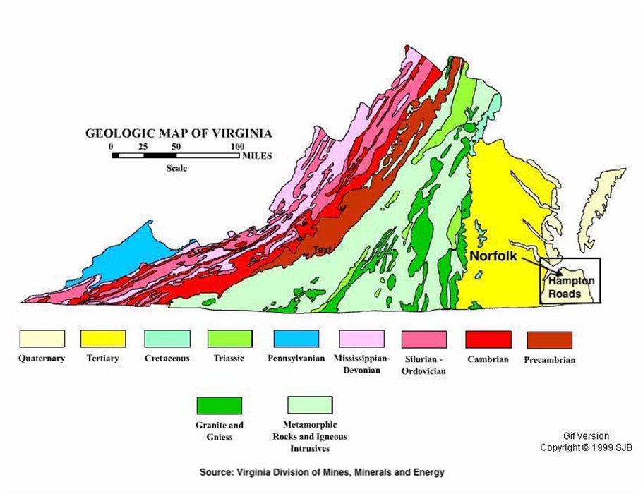
Geologic Map of Virginia.
The physiographic province is part of the Outer Coastal Plain shaped by changes of sea level and where unconsolidated sediments extend to depths of over 2,000 ft. Norfolk’s typography is flat (less than 3% slope), low in elevation, and dominated by dendritic drainage patterns consisting of creeks feeding rivers that drain into the Chesapeake Bay.
The region is experiencing an increase in the rate of coastal flooding caused by rising sea levels. The Virginian-Pilot has published numerous newspaper articles on how vulnerable the Tidewater region of southeastern Virginia is to a rising sea level. These media accounts have referenced sources identifying the tidewater area of Virginia as having the highest relative sea level rise (SLR) rate on the east coast. They also have identified the city of Norfolk (Figure 2) as one of the most exposed urban environments in the United States, second only to New Orleans. As an aid to its citizens, the city has developed a tool, TITAN (tidal inundation tracking application) for the public to see how a range of flood stages could encroach on their property. It is available at gisapp1.norfolk.gov/TITAN/.
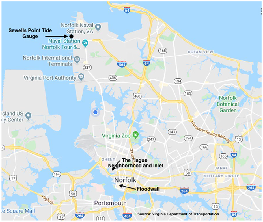
Map of Norfolk.
From a historic perspective, changes in sea levels have been relatively stable, and the Tidewater area has enjoyed imperceptible changes since the English settlement 400 years ago. However, for the first time in millennia, people are experiencing a global rate of change in sea levels that are disruptive to our way of life. We now face the potential for dramatic change within one lifetime (Plag, 2014).
An example which reinforces this perception is a study by the Virginia Institute of Marine Sciences (VIMS) that explains how SLR is increasing the region’s vulnerability to the impacts of storm surge (Boon, 2005). The study compares the impact of Hurricane Isabel in 2003 with an unnamed hurricane in 1933 using data recorded on National Oceanic and Atmospheric Administration (NOAA) Tide Gauge 8838610, Sewells Point, Virginia located at Naval Station, Norfolk (Figure 2). Even though the 2003 event produced a lower surge of 1.45 m (4.8 ft), the storm tide high water marks equaled those of the 1933 hurricane that produced a surge of 1.78 m (5.8 ft). Boon attributes the comparable impact of the lesser storm to the fact that sea levels in the region had risen some 0.30 m (1.0 ft) over the 70-year span between the two storms. In addition, historic data in The Hague neighborhood northwest of downtown Norfolk (Figure 2) shows an exponential increase in the number of hours of flooding from about 10 per year in 1930 to more than 200 per year by 2010 (Atkinson et al., 2013).
As a consequence, the region has experienced a gradual increase in coastal flooding. It has disrupted local traffic patterns, overloaded waste treatment facilities, and backed-up stormwater drainage systems. Studies have focused on how the extent and depth of coastal flooding will change and its impact as the sea level continues to rise. However, these studies have limited information on the duration of floods, how it will change over time and impact infrastructure.
Therefore, the objective of this article is to encourage an appreciation for the duration of coastal flooding along with an emphasis placed on the height and extent of storm surge. The aim is to develop guidance for determining durations sufficient for planning studies and simple designs, and a basis for more complicated projects that warrant more detailed analyses.
Literature Review
The objective of the literature review is to seek information on the duration of coastal flooding, how it could change over time, and ways to assess the risk of potential impacts on the type of infrastructure in Norfolk. The results are grouped (a) by the science of SLR, coastal flooding, and flood durations; (b) by the challenge of using historic data to project a future that is changing; and (c) the application of risk to assess impacts.
Duration of Coastal Flooding
NOAA (Sweet et al., 2014) examined the rising sea levels and the increase of occasional flooding defined as exceeding the elevation threshold for “minor” coastal flooding (nuisance level) established by the National Weather Service (NWS). It addressed three questions: (a) has historical SLR changed the frequency and duration of nuisance flood events, and the probability of nuisance flood events; (b) whether there are climatic patterns associated with year-to-year differences; and (c) whether nuisance floods occur during any particular season and why. NOAA used a meteorological year that runs from May to April to not split the winter season, the dominant storm season. They also used cumulative duration (hours) and number of days exceeding the nuisance flood-level threshold per year to estimate how it has changed over time.
The NOAA study concluded that the frequency and duration of nuisance-tidal flooding is intensifying and recurrence probabilities are compressing in a nonlinear trend; that is, lesser storm events will contribute to more frequent floods as exemplified in Boon (2005). It explains (a) how El Nino Southern Oscillations (ENSO) can create large year-to-year variability in sea levels; (b) that seasonal variation is regional; and (c) that the autumn season tends to dominate the Mid-Atlantic States.
Sweet and Park (2014) studied increases in annual exceedance probability (AEP) levels above minor (nuisance level) coastal flooding elevation thresholds established by the NWS for 27 U.S. coastal cities. They used the same NOAA- (Sweet et al., 2014) defined meteorological year to better identify anomalies during phases of the ENSO. The study notes tidal flood frequencies are typically higher along the Mid-Atlantic States during El Nino. A key finding is a nonlinear increase in flood frequencies that can lead to under estimating future projections. The main reason is the use of past trends is insufficient to reflect change in the future.
In an assessment for Norfolk, Sweet and Park (2014) used 0.53 m (1.74 ft) above mean higher high water (MHHW) levels as the threshold for minor (nuisance) flooding (0.88 m [2.89 ft], North American Vertical Datum of 1988 [NAVD 88]). Similar to NOAA (Sweet et al., 2014), the study limited its assessment to the number of daily floods above the threshold per year.
Sweet and Marra (2016) provided an update to the Sweet and Park’s (2014) paper, noting an increase of the number of days of nuisance flooding during the May 2015 to April 2016 meteorological year. During that period, a strong El Nino dominated the global climate and the frequency of nuisance flooding increased some 50% on average across all locations as compared to May 2014 to April 2015 period.
Cid et al. (2015) studied long-term trends in frequency, intensity, and duration of extreme storm surge events in the Mediterranean Sea and the North Atlantic Ocean. It developed a nonstationary, time-dependent statistical model combining the generalized Pareto distribution for events exceeding a threshold, and a nonhomogeneous Poisson process for assessing the occurrence rate for those events. It offers time-dependent 50-year return-period results for storm stage and intensity but only offers an increase or decrease in trends in duration (hours/year) using the durations of the extreme events.
NOAA (Sweet et al., 2017) provided updated scenarios of global mean sea level (GMSL) and integrating scenarios with regional factors contributing to sea level change for the U.S. coastline. It aligns six scenarios with emissions-based, conditional storylines and global model projects. The six scenarios with corresponding GMSL rise are Low (0.3 m), Intermediate-Low (0.5 m), Intermediate (1.0 m), Intermediate-High (1.5 m), High (2.0 m), and Extreme (2.5 m) by the year 2100. It includes the work of Sweet and Park (2014) and Sweet and Marra (2016) on nuisance flooding.
NOAA (Sweet et al., 2018) identified that coastal communities require consistent guidance on flooding. It offers a method to derive three coastal flood height impact thresholds and identifies the need for similar frequency-duration impact thresholds. The report notes as coastal cities plan engineered solutions, it is important to understand how the extent, depth, and duration of flooding will change and affect projects over the project’s life cycle.
In a companion document to the NOAA references, NOAA (Sweet et al., 2019) provided further evidence of an increasing frequency of high tide flooding (HTF) along the U.S. coastlines due to relative SLR. The report defines HTF as a height threshold ranging from about 0.5 m (1.6 ft) to 0.65 m (2.1 ft) above MHHW level and referred to as “nuisance” or “sunny day” flooding. In 2018, the national HTF frequency reached 5 days (median values). NOAA expects the HTF frequency to likely increase to about 7 to 15 days by 2030 and 25 to 75 days by 2050.
Moftakhare et al. (2018) offered a definition for nuisance flooding based on established flood intensity thresholds for flood consequences such as pedestrian safety, public property damage, and health risks. Based on a literature review, the authors recommended defining nuisance flooding using a NOAA’s National Ocean Service definition as “Flooding that leads to public inconvenience . . .” based on a depth >0.03 m and <0.10 m where the upper range “. . . corresponds to the 50th quartile of the observed (10 U.S. tide gauges) hourly water level above MHHW.” They note that emphasis is placed on extreme (infrequent) events, and the possibility of acute impacts of flooding. However, this article identifies the need to understand the increasing impacts of chronic flooding (relatively frequent and small-magnitude events) such as discussed by Atkinson et al. (2013). It recommends measuring nuisance flooding “. . . in the number of hours that coastal water levels are above height thresholds that trigger the onset of flooding.”
Stationarity versus Nonstationarity of Data
The American Society of Civil Engineers (ASCE, 2018) provides a method of practice (MOP) for the design of climate resilient infrastructure. The MOP presents methods to update and describe a changing climate over the life cycle of infrastructure. The document references NOAA (Sweet et al., 2014) and its recommendations to estimate the current impact and how it has changed over time using cumulative duration (hours) and number of days exceeding the nuisance flood-level threshold per year.
The first key aspect of the ASCE MOP is a distinction between stationarity, an assumption that statistical properties of climate extremes in the future will be similar to those from the past; and nonstationarity, where future statistical properties will vary substantially. In the past, engineers could depend on a consistent statistical mean and variance over the life cycle of infrastructure; in the future, the values are time variant.
Nonstationarity has long been an issue with analyzing fluvial flood stages. Read and Vogel (2015) demonstrate that over a 100-year period, watersheds often have forests cleared, land converted to farms, and later developed into communities; and rivers are altered by the construction of dams, bridges, and channels. Such anthropomorphic impacts alter runoff patterns, sediment transport, and flow velocities. The result is annual peak flow records that are based on statistical properties that can vary significantly.
Read and Vogel (2015) used a log-normal 2 analysis to simulate future fluvial floods associated with a particular design event under nonstationarity conditions. They used factors to represent hydraulic variability and increasing trends in the magnitude of floods. These authors assessed a range of flood events coupled with an increasing range of flood flows. The results show where there is stationarity, the probability density distribution for return periods has an exponential shape. Where there is nonstationarity, the distribution takes a more normal or symmetrical shape.
Risk
A key point made by Read and Vogel (2015) is that for the design of infrastructure, the probability of failure (or reliability) over its lifetime “. . . is perhaps the most important piece of information an engineer can communicate to planners and the public.” They explain how in 1983 the U.S. Army Corps of Engineers (USACE) adopted risk-based design principles to select a level of protection based on minimizing annual damage costs from a hazard.
Risk is a function of failure probability and consequences. Failure probability is a product of the AEP of the hazard and the probability of failure of the infrastructure during the loading function. The consequences are a combination of the potential for loss of life and direct and indirect economic losses. Kamphuis (2010) offers a range of design failure probabilities based on a failure type and the seriousness of the consequences for coastal infrastructure. For damages, probabilities range from 10−3 to 10−7, and for loss of life, the range is 10−5 to 10−7.
Linkov et al. (2016) expands the risk concept to include resilience. Where risk communicates the potential for loss, resilience defines the ability of a system to recover and adapt in response to a loss. Pezza and Pinto (2019) offer insights for related decision theory specific to coastal infrastructure.
The USACE (2018) performed a coastal storm risk management study of the city of Norfolk. Included in the study was as assessment of time needed to close proposed storm surge barriers during a coastal tidal surge. The study used Hurricane Sandy as a storm of record for the longest duration for flood elevations that equaled or exceeded 4 ft (1.2 m), NAVD 88. As noted in the study, The closing of the storm surge barrier is expected to occur during a preceding low tide in order to maximize interior storage for rainfall runoff. The water surface elevations associated with Hurricane Sandy were then analyzed to calculate the expected time duration from the preceding low tide, through the storm event, and until the water surface elevations dropped below 4 feet.
The gate closure duration is expected to increase due to rising sea levels from 4 days in 2026 to 5 days in 2050 to 5.5 days in 2075.
Summary
In summary, there is discussion in the literature where the recommendation is to use the cumulative duration (hours) and number of days exceeding the nuisance flood-level threshold per year to represent the duration of coastal flooding. Absent in the literature is a definitive way to assess nonstationarity and the translation of this data into the AEP for individual events needed for the use of risk-resilient analyses. As a result, also absent is the use of flood duration frequencies to quantitatively assess impacts on infrastructure.
This article explores how rates of tide durations could change over time and offers insights on how increasing flood durations could qualitatively impact infrastructure in the city of Norfolk. The analysis uses a baseline elevation matching an existing floodgate sill and a simple analysis to determine flood duration AEP curves for the 50%, 10%, 4%, 1%, and 0.2% return periods. The results are combined with an SLR scenario to determine how the duration for each set of predicted annual probability exceedance levels change over time.
AEP Analysis
The authors chose to use a peak over threshold (POT) methodology to assess the annual probability of exceedance levels; data deemed necessary to assess the impact on infrastructure. They used the Norfolk Floodwall located along the Elizabeth River in downtown Norfolk, Virginia, to select a threshold elevation to assess the annual probability of exceedance levels for flood durations. The wall was built in response to two 1933 hurricanes that hit the area and caused extensive flooding throughout the inner city streets.
In the 1960s, the USACE and the city of Norfolk designed and constructed the floodwall to protect the downtown business and commercial districts. The floodwall alignment (Figure 3) is 611-m (2,000 ft) long and consists of a combination of concrete walls, floodgates, and a pump station to collect and discharge interior drainage and any storm surge overtopping the wall.
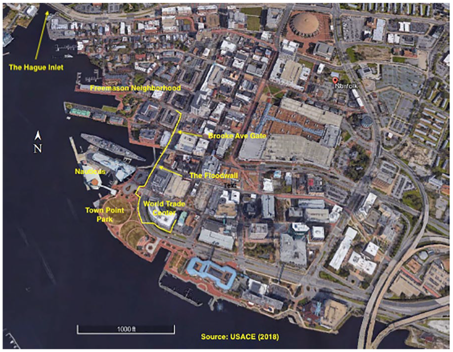
Map of Downtown Norfolk.
For this study, the authors selected the Brooke Avenue Floodgate to define the threshold elevation needed to determine the annual probability of exceedance levels for flood durations. The gate is a steel horizontal rolling street closure stored in a pocket in the floodwall (Figure 4). The top of the gate is at elevation 11.52 ft, NAVD 88 (92). The gate and wall were designed to provide three feet of freeboard for the 1933 storm of record.
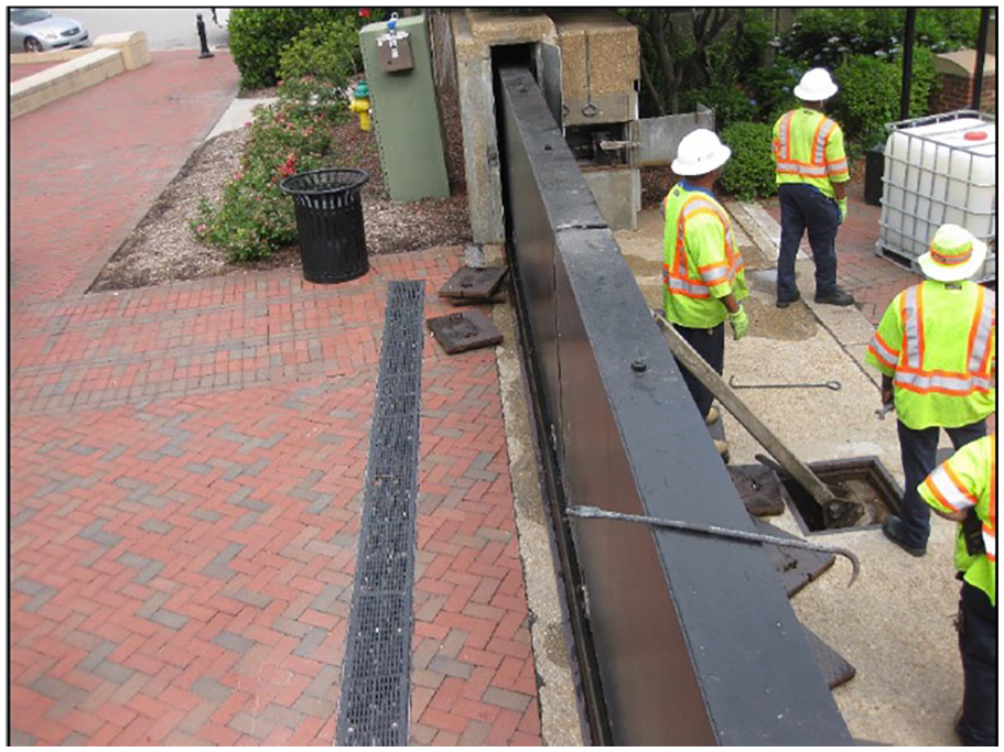
Brooke Avenue Steel Gate (USACE, 2018).
It has the lowest sill elevation of all the gates at 1.53 m (5.00 ft), National Geodetic Vertical Datum of 1929 (NGVD 29) as identified on record drawings. As part of a 2012 Federal Emergency Management Agency (FEMA) flood certification application, the city converted the NGVD 29 datum to the NAVD 88 datum by minus 0.27 m (0.9 ft) (Fugro Atlantic, 2012). The revised sill elevation is 1.25 m (4.10 ft) NAVD 88 (92) and its purpose is to prevent water levels above this elevation from entering into the downtown area.
The authors selected the sill as the threshold elevation for the POT analysis. The city starts to see damages occur when tide elevations approach this sill elevation. When weather forecasts predict tides exceeding this elevation, the city closes all gates and staffs the pump station to remove stormwater that may collect interior to the wall alignment.
The (92) following the reference datum is the year the city converted its vertical datum to NAVD 88. Since that time, the National Geodetic Survey (NGS) has made adjustments resulting in a difference of 0.009+ m (0.03+ ft) over the past 26 years (K. Marchello, personal communication, October 11, 2018, 2018). However, since the gate sill was physically surveyed in 2010, the authors chose to ignore any possible difference that may have occurred over the past 8 years.
The data analyses used NOAA Tides and Currents verified hourly height water levels for 8638610 Sewells Point, VA tide gauge starting with the initial reading July 1, 1927, to May 31, 2018. The gauge is located on Naval Station Norfolk (Figure 2). The location is such that the influence of river and hydrology is likely negligible compared with the tide and surge (T. Ezer, personal communication, January 24, 2020). These data are the oldest available record in the greater Hampton Roads Harbor and were used for the original design. These analyses used data based on the NAVD 88 vertical datum and are available at: https://tidesandcurrents.noaa.gov/waterlevels.html?id=8638610&units=standard&bdate=19600101&edate=19601231&timezone=LST&datum=MLLW&interval=h&action=data.
The analyses used EXCEL spreadsheet as a simple way to sort the historic tide data into annual records. A full record is 8,760 hours per normal year with 8,784 hours for a leap year. Not all annual records are complete.
The analyses are based on the following steps:
A storm event is defined as any time the tide equals or exceeds elevation of the Brooke Avenue gate sill elevation of 1.25 m (4.10 ft) NAVD 88.
Used NOAA’s relative sea level trend of rise of 4.62 ± 0.22 mm/year as of June 27, 2018. The data are available at: https://tidesandcurrents.noaa.gov/sltrends/sltrends_station.shtml?id=8638610.
Created stationarity by adjusting historic tide data from 1927 to 2017 to equal 2018 levels by adding the SLR trend times the number of years between the year of record and 2018. For this case, stationarity means the historic tide records were adjusted to reflect no change in sea levels for the past 90 years. The purpose of this adjustment is to create a “current record” of all tide data as if it occurred on May 31, 2018.
Projected future stationarity by assuming a “bathtub” affect and adjusting the “current record” by increments of 0.15 m (0.5 ft), 0.30 m (1.0 ft), 0.45 m (1.5 ft), 0.60 m (2.0 ft), and 0.75 m (2.5 ft) to create future records of all tide data. The bathtub affect is a first-order estimate of storm surge based on a static increase in water level. It is a simplistic assumption because the dynamics of coastal flooding are nonlinear. However, it offers a clear way to communicate water levels to the public.
The number of events that the tide equaled and/or exceeded the gate sill elevation is checked each year. For each event, the number of continuous hours each tide event equaled and/or exceeded the gate sill elevation is counted. Duration, Dt, is defined as the total number of continuous hours per tide event that equaled or exceeded the specified elevation.
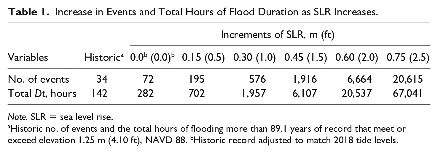
Table 1 shows how the historic number of events and total duration in hours exceeding the threshold could change as the increments of SLR increase.
Increase in Events and Total Hours of Flood Duration as SLR Increases.
Note. SLR = sea level rise.
Historic no. of events and the total hours of flooding more than 89.1 years of record that meet or exceed elevation 1.25 m (4.10 ft), NAVD 88. bHistoric record adjusted to match 2018 tide levels.
In assessing the data, one would expect a correlation between the flood elevation and duration. There appears to be a linear relationship, but greater storm magnitudes do not necessarily relate to longer flood durations. It is the time the tide cycle lingers that controls the durations, not the peak elevation of the storm event. The effects of extra-tropical storms tend to have lower magnitudes but linger through multiple tide cycles, whereas tropical storms display the opposite characteristics. A possible driving function is how the ENSO creates year-to-year variability in sea levels (Sweet & Park, 2014). For example, the year 2009 has the historic record for most events and the largest total hours of flooding, and the year 1972 has no historic record exceeding the threshold. However, at the 0.45-m (1.5 ft) increment of SLR, 1972 has more events, and at the 0.60-m (2.0 ft) increment, 1972 has higher total hours of flooding.
Another characteristic of the data is shown in Figure 5, which compares the probability mass distribution (PMF) for the historic data with the adjusted data. The historic data takes the shape of a geometric distribution more aligned with a normal distribution characteristic of nonstationarity as described by Read and Vogel (2015). The adjusted data converges to an exponential shape more representative of stationarity.
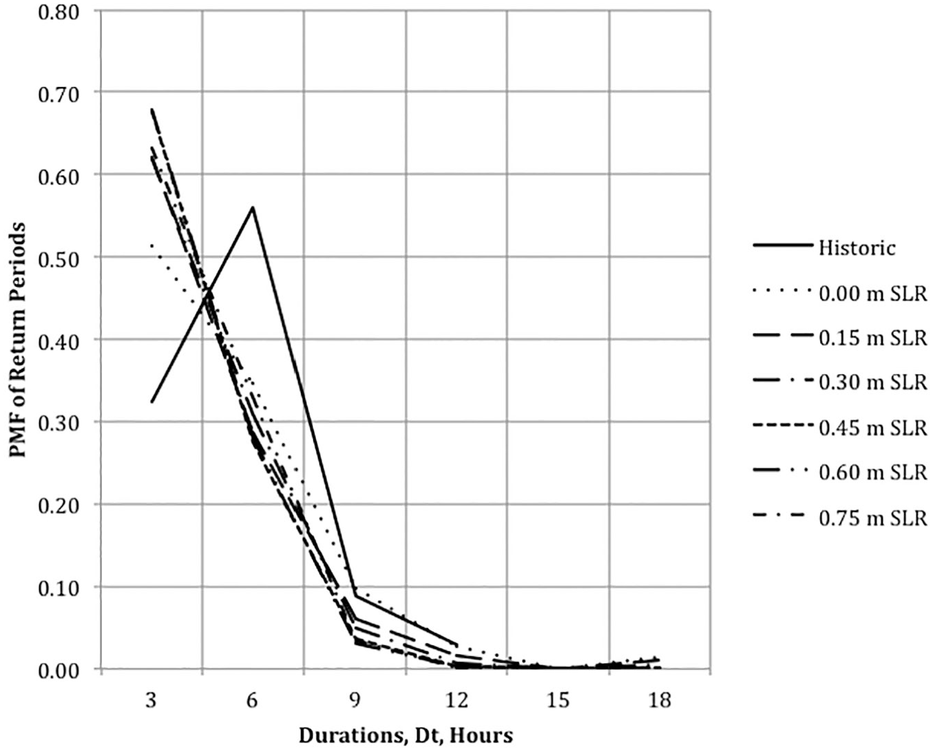
PMF distributions of return periods truncated at 99% CMF.
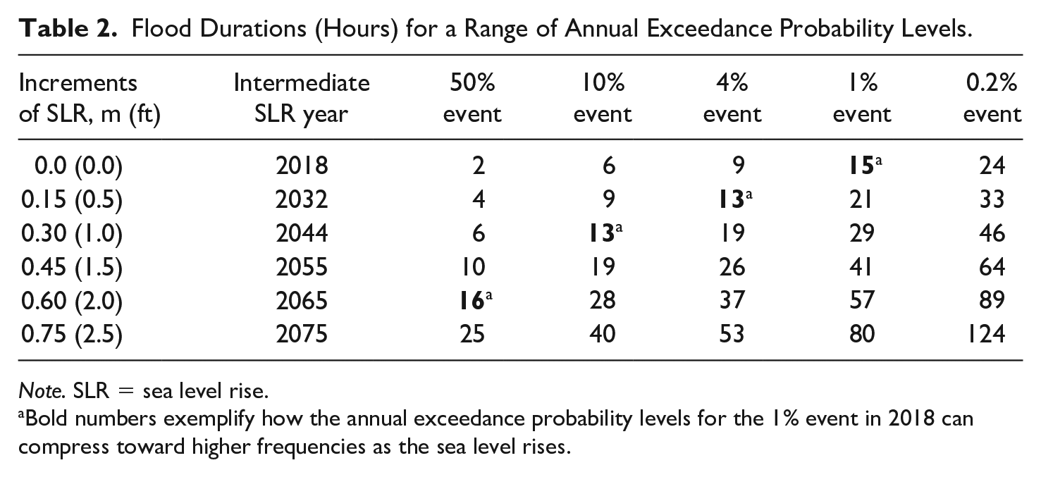
For a timeline, the authors selected the U.S. Global Climate Change Research Program (NOAA, 2018) Intermediate SLR scenario as a reasonable representation of the potential for higher sea levels. The scenario is based on the USACE Sea Level Change Curve Calculator (2017.55) available at corpsmapu.usace.army.mil/rccinfo/slc/slcc_calc.html, retrieved July 3, 2018. The timeline is combined with the results in Table 2.
Flood Durations (Hours) for a Range of Annual Exceedance Probability Levels.
Note. SLR = sea level rise.
Bold numbers exemplify how the annual exceedance probability levels for the 1% event in 2018 can compress toward higher frequencies as the sea level rises.
The probability analysis is based on the assumption that the exponential distribution of transformed tide data represents stationarity. The authors selected the POT method (Kamphuis, 2010) to tally the number of flood events that meet or exceed the Brooke Avenue gate sill elevation. The probability is computed using a Poisson discrete probability distribution based on an infinite number of repeated trials with binomial outcomes (Bernoulli trials). The expected value is
This analysis requires that the individual data points are statistically independent. As a means to manage independence between hourly data points, the data points are grouped into those hours that continuously met or exceeded the gate sill elevation. The total duration for each group represents a flood event that exceeds the threshold.
Probability is based on a binomial distribution where lambda, λ, represents the number of events that equal or exceed the threshold that can occur per year. For this analysis, records cover 91 years. Given that there are a few data gaps, λ equals the total number of hours of data divided by the total number of hours that makes up 1 year of complete data or 780,197 hours by 8,760 hours per normal year, which equals 89.1 years of data. For the POT analyses, the minimum unit of duration is 1-hour, and the bin limits are in increments of 3 hours.
The first assumption is that the historic tide cycles are representative of future tide cycles. It is reasonable to expect the cycles to remain diurnal, but the conditions that drive future storms are likely to be different. The second assumption is each event is independent, that is, the cause for the incident is not influenced by the previous incident. This is truer where there is more time between incidents. The third assumption is each event is unbiased, that is, equal forces cause each incident. This is truer the less time there is between incidents. The fourth assumption is λ is constant over the full range of data, which is a simplification to facilitate the use of the Poisson methodology.
The POT generates a cumulative distribution of the duration on the x-axis versus probability on the y-axis. This distribution was transformed into normal, log-normal, Gumbel and Weibull distributions to determine which method offered the best linear progression. The log-normal distribution provided the most consistent results.
Figure 6 is an example, a plot of the 0.45-m (1.5 ft) increment of SLR. This increment results in 1,916 events of duration over a period of 89.1 years that exceeded the threshold. The equation for computing Dt for a range of annual probabilities of exceedance above the threshold is based on an equation (4.9) used by Kamphuis (2010) to compute the “
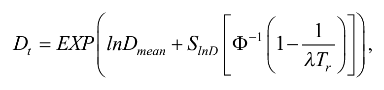
where
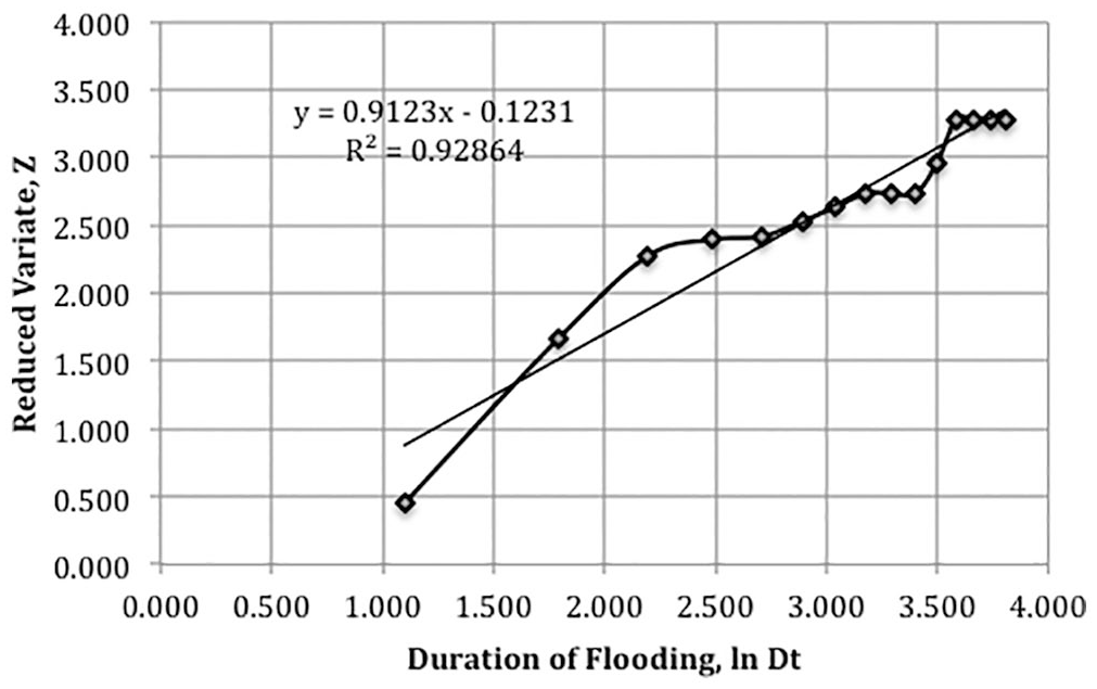
Log-Normal distribution for 0.45-m (1.5 ft) increment of SLR.
Results
The analysis calculated flood duration AEP curves for the 50%, 10%, 4%, 1%, and 0.2% return periods. The exponential trend line best fits the events. EXCEL uses an exponential least squares fit to data based on
The computations are summarized in Table 2. The ±90% confidence intervals are not included; however, as an example, the range for the 1% event is ±5 to 8 hours as the SLR increment increases from 0.0 to 0.75 m (2.5 ft).
Figure 7 plots the NOAA (Sweet et al., 2017) Intermediate SLR scenario versus the computed duration values in Table 2 for each AEP. The NOAA Intermediate SLR Scenario is aligned with emission-based and global model projections for a GMSL rise of 1.0 m by the year 2100.

Durations for a range of AEP levels for the NOAA Intermediate SLR scenario.
Figure 7 offers a means to understand how the magnitude of possible change could happen based on the NOAA Intermediate SLR scenario. It would help engineers anticipate possible impacts to infrastructure and judge appropriate mitigation measures. For example, the bold numbers in Table 2 and the data points in Figure 7 show how the 1% event compresses over time; in the figure, the 1% event (15 hours) in 2018 becomes more like a 10% event between 2044 and 2055 or about 2048. For the NOAA Intermediate-High (GMSL rise of 1.5 m) and High SLR (GMSL rise of 2.0 m) scenarios (not shown), the 1% event (15 hours) would compress to the 10% event by about 2042 and 2037, respectively.
Numerical analyses would be necessary for project-specific computations. Castrucci and Tahvildari (2018) performed hydrodynamic modeling using Delft3D (an open source software developed by Deltares, an indepenent institute for applied research available at deltares.nl/en/) to study the vulnerability of critical flood-prone neighborhoods in the Hampton Roads area. One location was the same Hague neighborhood (Figure 2) noted above located about 0.4 miles northwest of the Brooke Avenue gate.
The analysis computed the extent, intensity, and duration of storm surge inundation under different SLR scenarios. Flood duration was defined as the time over which the model predicted the presence of water over an area, that is, once the total water level (storm surge + tide + SLR) was higher than the elevation of the point under study. Flooding ended once the water level subsided and reached a value that was constant over time.
The authors compared the computational results with the bathtub approach. The numerical analysis shows that the extent of flooding is less and as a result, the duration of flooding is less. Therefore, this conceptual POT analysis is more likely conservative in estimating flood durations.
Limitations
As noted in the introduction, the objective of this article is to encourage an appreciation for the duration of coastal flooding along with an emphasis placed on the height and extent of the surge. As identified in the literature review, there is an absence of a definitive way to assess nonstationarity and the translation of these data into the AEP for individual events needed for the use of risk-resilient analyses. Also absent is the use of duration frequencies to quantitatively assess impacts on infrastructure. Therefore, the article offers guidance for determining durations sufficient for planning studies and simple designs, and a basis for more complicated projects that warrant more detailed analyses.
However, the use of Poisson discrete probability distribution is a simplification and is used as a method to generate an example of duration curves. The assumptions for future tide cycles, independence, nonbias, and a constant annual rate of change are necessary to use the binomial methodology.
The authors emphasize the need for the scientific community to develop a rigorous, peer-reviewed methodology to compute annual exceedance probabilities for a range of storm events. NOAA offers an inundation analysis tool available at https://tidesandcurrents.noaa.gov/inundation/AnalysisParams?id=8638610. Adding the ability to statistically predict possible AEP for storm durations to the tool would be a great benefit for planning phase studies of a project. It would offer a baseline for the more detailed engineering phase studies needed to assess the impact of future storm conditions over the life of infrastructure systems.
Potential Impacts to Infrastructure in the City of Norfolk
Along with the extent and stage of flooding, the duration of flooding can impact the performance of infrastructure. The following discussion offers a qualitative assessment of how increasing flood durations impact the Brooke Avenue gate, Norfolk Floodwall, and other forms of infrastructure systems in the city of Norfolk (Figure 3). For quantitative assessments, research is needed to assess how increasing durations of flooding affect the fragility of infrastructure and link it with risk assessments. Adding this variable to failure mode analyses will help identify how longer flood stages could impact performance and whether it is an important factor in design and risk-resilient analyses.
As noted in the introduction, the authors selected the Brooke Avenue gate sill as the baseline for the POT analysis. It is obvious the increase in flood durations will result in a need to keep floodgates closed for longer periods. Listed below are how longer duration gate closures will affect operations:
Longer durations will increase operations and maintenance costs. The floodwall system is robust, but it was designed for periodic usage. Extended periods of deployment may result in increased wear of gate components that would necessitate the need for overhaul of the system at more frequent intervals.
City facilities located on the flood side of the floodwall would not be available for operations. The city operates the National Maritime Center NAUTICUS and a cruise ship terminal, which are a major engine for much of the city’s tourism economy. Having to keep these facilities closed for any length of time would affect revenues and trickle down business in the downtown economy.
The city hosts numerous festivals, cultural events, and celebrations on the downtown park spaces of Town Point Park. In many ways, this park defines the city from a cultural perspective. A large portion of the park is located in areas subject to flooding and accessible through the floodgate system.
The closure of Brooke Avenue gate would impact the flow of traffic in and out of the Freemason neighborhood and adjacent businesses.
The logistical supply access to the World Trade Center is through a floodgate on the levee system. Extended closures would impact operations and the reputation the building maintains.
As for the floodwall, extended flooding durations would have a negative impact in the following ways:
Longer durations will extend pumping of storm water. The system was designed to allow larger storms to bypass during normal tidal conditions. During an extended tidal event, pumps would be the only mechanism to evacuate storm over wash and precipitation from the downtown area. This would increase the risk of interior flooding at City Hall Avenue and Boush Street affecting several commercial buildings, parking facilities, and multiresidential buildings.
Longer flood durations increase the risk for greater infiltration into the downtown wastewater collection and conveyance system. During extended tidal departures, the system could become vulnerable, particularly with a higher head imparted by the tidal waters. This may result in both high flows to treatment plants and the likelihood of overflows in the system.
Higher and extended tides could ultimately impact the structural stability of the wall. The wall is a concrete I-wall bearing on piles and a steel sheet wall to cutoff under seepage and increase global stability. Extreme tides in both magnitude and duration will increase loads on the wall system and increase under seepage that will reduce the global stability of the wall system not anticipated during the original design.
For the city in general, flooding that exceeds elevation 1.2 m (4 ft), NAVD 88 is a tipping point where following impacts start to affect the quality of life:
Extended flooding from tidal events would have serious impacts on the City’s storm water collection and conveyance systems as the performance of the system would drop off due to the increased tailwater conditions. Precipitation flooding would aggravate the flooding throughout the City, particularly in lower lying neighborhoods. The likelihood of flooded homes would increase.
As noted above for the downtown area, longer flood durations increase the risk for greater infiltration into the citywide wastewater collection and conveyance system. In 2009, inflows to a regional wastewater plant treatment located in Norfolk exceeded 90% of peak flows for three consecutive months in a row, triggering a state review to determine requirements for increased capacity.
Transportation networks, including roadways and light rail would also be negatively impacted. Much of the roadways are susceptible to flooding. With an inability to use roadways, economic activity is slowed in the immediate situation. Several sections of the Norfolk Tide light rail system are vulnerable to flooding from both tidal and precipitation flooding. Once water reaches a specific height, the light rail system is shut down and over-road bridges for buses would need to be utilized.
Roadway conditions would rapidly deteriorate as road subbase and subgrades are saturated for extended times. Many areas have clay and silt in-situ soils and would weaken during saturated conditions causing base failure and numerous pavement condition issues. This would increase costs for road maintenance.
Other subterrain infrastructure would likely deteriorate at a much higher rate, as floodwater would subject underground utilities to a corrosive environment higher than expected during design, accelerating the need for replacement. Long-term inundation would also subject buried infrastructure to unanticipated structural loading.
City beaches would experience increased erosion and, as a result, increase the need for higher and more frequent beach nourishment projects.
The perception that flooding has reached a tipping point in the area could eliminate economic development and exacerbate the ability for the city to recover.
A critical point to understand is how the magnitude of possible change in flood durations could impact a project. In assessing alternatives, the city is considering installing a low wall around The Hague Inlet (Figure 2) to about the same elevation as the Brooke Avenue gate sill. Based on the Intermediate SLR scenario, Figure 7 shows how the 1% event in 2018 becomes the 10% event by about 2048. Having this additional information would help planners and designers assess how flood durations impact the fragility of infrastructure and whether it is an important factor in risk-resilient assessments.
Conclusion
Coastal communities are experiencing a gradual increase in coastal flooding. It has disrupted the function and operations of various forms of infrastructure. Studies have focused on how the extent and depth of coastal flooding will change as sea levels rise. However, there is limited information on how the duration of coastal flooding will change; specifically, in a format needed to support risk assessments.
In the absence of an accepted methodology to assess flood durations, the authors used a simplified procedure to develop flood duration frequency curves. The analysis uses historic tide data from the Sewells Point tide gauge in Norfolk, Virginia, which exhibits nonstationarity because of rising sea levels. The authors translate 90+ years of data to match 2018 sea levels to simulate stationarity and combine the data with increments of rising sea levels to represent future tide elevations. Assuming stationarity enables the use of a Poisson discrete probability distribution to calculate the annual probability of exceedance levels for flood durations for a specified threshold level and how those durations and probabilities could change over time.
The methodology has limitations and the results are likely conservative. Such results are appropriate for planning phase studies; however, computational methods are more suitable for engineering phase studies to assess the impact of future storm conditions over the life cycle of infrastructure systems.
The article concludes with a qualitative assessment of how increasing flood durations impact the Norfolk Floodwall and infrastructure systems in the city of Norfolk. It gives an example of a proposed alternative at The Hague Inlet and how the compression of the flood duration frequency over time could provide insights to risk informed analyses.
The article identifies a need to research what influences the variations in tide cycles. In addition, there is a need to present historic data as displaying nonstationarity similar to work by Read and Vogel (2015). In addition, the authors recommend adding this capability to NOAA’s inundation analysis tool. The site could provide curves as shown in Figure 7 for each tide gauge for a range of SLR scenarios. It would offer municipalities such as Norfolk an economical tool to quickly assess the impact of flood durations over time along with the stage and extent of coastal flooding. In addition, research is needed to assess how duration affects the fragility of infrastructure and link it with risk assessments. This research would expand the understanding of the hazard of rising seas, enhance failure mode analyses of infrastructure, and make for better-informed risk-resilience assessments for planners and engineers.
Footnotes
Declaration of Conflicting Interests
The author(s) declared no potential conflicts of interest with respect to the research, authorship, and/or publication of this article.
Funding
The author(s) received no financial support for the research, authorship, and/or publication of this article.
