An efficient algorithm for high utility sequential pattern mining over data streams based on sliding window model

Abstract

In the era of the digital economy, the exploration of useful knowledge from data streams has garnered significant attention due to its wide-ranging applications. However, the rapid and infinite nature of data streams poses challenges for efficiently mining high utility sequential patterns, including strong spatio-temporal constraints and the combinatorial explosion of sequence data search spaces. To address this and adapt to a variety of application scenarios, this paper delves into the investigation and design of an efficient algorithm for high utility sequential pattern mining over data streams based on the sliding window model (HUSP_DS). This algorithm utilizes a projection mechanism within a sliding window to recursively search for all interesting patterns. Additionally, it introduces a novel structure called the dynamic utility index table, which stores information such as the utility and index positions of data stream sequences. Notably, this structure proves highly effective in recursive search processes and utility updates. Comprehensive experimentation, conducted on both real-world and synthetic datasets, have shown that the superior performance of the HUSP_DS algorithm compared to state-of-the-art algorithms. This superiority is particularly evident in terms of temporal and spatial efficiency. Furthermore, the algorithm demonstrates suitability for mining sliding windows of arbitrary sizes, showcasing stable scalability.

Keywords

pattern mining data streams sliding window high utility sequential patterns sequence data

1 Introduction

High utility sequential pattern mining (HUSPM)¹ has emerged as a research hotspot in the field of data mining in recent years. Its primary goal is to discover valuable and interesting patterns from sequence data, which greatly aids business decision-makers in understanding and responding to customer behavior. HUSPM considers both the utility factor and the relative order of each sequence, making it more valuable for decision-making compared to traditional sequential pattern mining (SPM).^2,3 Furthermore, extracting implicit information from dynamically changing data streams has become increasingly important, as real-world data is often generated in continuous, infinite sequences in real time. Examples of such data include sensor networks, web clickstreams, satellite signals, and stock transactions, all of which are presented as data streams. The technology of mining high utility sequential patterns (HUSPs) from data streams has thus become an important technique in the field of pattern mining. Traditional high utility sequential pattern mining algorithms are mostly designed for static data and cannot handle real-time data streams. Additionally, the massive and rapidly arriving nature of data streams presents significant challenges for mining high utility sequential patterns within limited time and memory resources. Currently, data stream processing typically employs window models to continuously process segments of the data stream. Windows address the infinity of data streams by limiting the algorithm's operations to the window's scope, mainly targeting recent sequence data.⁴ Depending on the processing method, window models are classified into landmark windows, damped windows, and sliding windows.⁵ Sliding windows and landmark windows process only a certain amount of recent data, treating all data within the window equally. However, compared to sliding windows, landmark windows may lose data at the window boundaries, leading to information bias.⁶ Damped windows assign different importance to data based on insertion time, but they require processing all data, resulting in significant computational overhead.⁷

Several high utility sequential pattern mining algorithms for data streams have been proposed to handle sequential data streams. These algorithms use different window models and data structures to mine high utility sequential patterns from data streams. MAHUSP⁵ algorithm uses a landmark window to mine high utility sequential patterns from data streams. It employs memory-adaptive mechanisms of SBMA and LBMA to find result sets within limited memory resources. However, it is disadvantageous for time-sensitive data, as important events occurring at window boundaries may be overlooked, and its ability to detect burst or irregular events is poor. Additionally, the SBMA mechanism's long runtime for dense datasets results in low algorithm efficiency. HUSP-Stream⁸ algorithm uses a sliding window model to process data streams. The HUSP-Tree structure used in this algorithm is not suitable for long-term information storage because its main idea is to facilitate the update process when new transactions enter or leave the window. This data structure is ineffective for mining HUSPs over the entire data stream, as it consumes more memory. Sliding windows are widely used due to their emphasis on recent data and limited memory usage,^9,10,11 HUSP-UT¹² algorithm uses a sliding window model to mine high utility sequential patterns from data streams. It employs the UT-Tree (Utility on Tail Tree) structure to update and maintain the utility information of data stream sequences. Using a pattern growth approach, it can mine high utility sequences by scanning the dataset only once. However, when dealing with large, dense data streams, the UT-Tree requires frequent updates to its leaf nodes, necessitating multiple traversals from the root node, leading to significant time and memory overhead. RStreamHusp¹³ algorithm is a concise pattern mining algorithm for data streams that uses a sliding window model to mine regularly occurring patterns in data streams. The DSRHUS-Trie structure is used to store utility information of sequences within the window. To determine whether a pattern is a high utility sequential pattern, it requires traversing each node from the root and calculating the sum of utility values in the utility array, resulting in significant time overhead.

Motivation: Although existing high utility sequential pattern mining algorithms can effectively process data streams, they still face the following challenges: (1) Data streams are typically high-speed, continuous, and infinite. Storing all data records in memory and processing each new incoming data record in real-time is impractical. Once data records are deleted, they cannot be retrieved from previous windows for searching. Therefore, designing a compact data structure to store both new and old data while updating the utility information of sequence elements is a crucial issue in the mining process. (2) Most previous work focuses on mining static sequence databases, and such algorithms cannot mine patterns from real-time changing data streams. Furthermore, existing HUSPM algorithms for data streams suffer from high temporal and spatial complexity, leading to inefficient mining. Hence, designing a high temporal and spatial efficiency HUSPM algorithm for data streams is essential to quickly discover interesting patterns within limited time and storage resources. (3) Most existing algorithms tend to generate a large number of candidate items during the mining process, including candidate sequences that do not exist within the current window. This results in significant memory consumption. Therefore, reducing the number of candidate items and narrowing the search space is an urgent problem that needs to be addressed.

Contributions: To address the aforementioned challenges, this paper presents a sliding window-based algorithm for mining high utility sequential patterns over data streams. Therefore, the main contributions of this study can be summarized as follows:

(1)
Dynamic data structure. To record utility information of sequences in real-time changing data streams, we designed a compact and dynamic utility index table (DUI-table). This data structure is dedicated to storing and maintaining the utility information of sequences within the sliding window.
(2)
Efficient algorithm. An efficient algorithm for high utility sequential pattern mining over data streams (HUSP_DS) is proposed, leveraging the DUI-table. The algorithm employs a projection mechanism within a sliding window to rapidly mine high utility sequential patterns in a data stream environment. The projection mechanism within the window uses a pattern growth approach, which effectively reduces the number of candidate items generated.
(3)
Sufficient experimentation. Extensive experiments, conducted on both real and synthetic datasets, affirm the high spatio-temporal efficiency and stable scalability of the proposed algorithm. The results demonstrate the algorithm's effectiveness in mining high utility sequential patterns within a data streams environment.
The following sections of this paper are structured as follows: Section 2 provides an in-depth review of existing high utility sequential pattern mining algorithms, with a specific focus on those tailored for data streams. Section 3 introduces and elucidates the essential definitions related to HUSPM. Section 4 introduces the algorithm proposed in this article. Section 5 conducts a rigorous evaluation of the proposed algorithm through extensive experiments on real and synthetic datasets. Section 6 summarizes the key findings and insights from the entire paper and initiates a discussion on potential avenues for further research.
2 Related work

2.1 High utility sequential pattern mining

High utility sequential pattern mining involves extracting valuable information from data by considering both the order and utility factors of sequences. In 2010, Ahmed et al.¹⁴ introduced two novel data structures, UWAS-tree and IUWAS-tree, tailored for mining web log sequences in static and incremental databases. While this algorithm eliminates the need for multiple database scans, it falls short in supporting sequence elements with multiple items, limiting its applicability to relatively simple scenarios. Following this, Ahmed et al.¹⁵ proposed two additional algorithms: the UL (Utility Level) algorithm, employing a layer-by-layer search, and the US (Utility Span) algorithm, relying on pattern expansion. The UL algorithm, however, generates a large number of candidate sequences through layer-by-layer candidate sequence generation and testing, with the number of database scans contingent on the maximum length of the candidate sequences. The US algorithm, on the other hand, is time-consuming due to its requirement for multiple database scans. In 2011, Shie et al.¹⁶ presented the UMSP algorithm based on MTS-tree for mining mobile sequence data. This algorithm utilizes depth-first search and breadth-first search methods to extract mobile sequence patterns with high utility values. However, these algorithms are limited to mining simple sequence data and struggle with handling complex time series data. Additionally, the utility values defined by these algorithms are uncertain and not well-suited for general mining frameworks. To address these limitations, Yin et al.¹ formally defined the general model of HUSPM for the first time. They proposed the USpan algorithm based on a utility matrix, employing a depth-first approach based on a lexicographic q-sequence tree to mine all high utility sequential patterns. However, the algorithm's spatio-temporal efficiency is hindered by the insufficient compactness of the upper bound SWU used in the algorithm.

Aiming at the difficulty of setting the minimum utility threshold, Yin¹⁷ et al. proposed a high utility sequential pattern mining algorithm TUS for mining the top-k items, using two threshold raising strategies and a pruning strategy to prune unpromising items, effectively improving the mining efficiency of the algorithm. In 2015, Alkan¹⁸ et al. proposed a data matrix structure and pruning strategy based on the cumulated rest of match (CRoM) upper bound. However, this algorithm requires a large amount of memory to store sequences and is not suitable for processing large data. In 2016, Wang¹⁹ et al. proposed a more efficient high utility sequential pattern mining algorithm, HUS-Span, which uses more compact upper bounds PEU and RSU to reduce the search space, and uses a utility linked list structure to store sequence utility information, although it reduces the algorithm running time, it also increases memory consumption. In 2020, Gan²⁰ et al. proposed the projection-based high utility sequential pattern mining algorithm ProUM. This algorithm designed a new utility upper bound SEU and used a more compact utility array to store sequence information. And it adopts depth-first search manner recursively mines high utility sequential patterns. Therefore, this algorithm performance is significantly better than USpan and HUS-Span. In order to further improve the mining efficiency, Gan²¹ et al. proposed the HUSP-ULL algorithm, which uses the lexicographic q-sequence tree and the utility linked list (UL-list) structure to store the utility information of each sequence. HUSP-ULL has good performance in mining large sequence data, especially datasets with a large average number of elements per sequence or a large average number of items per element. In 2020, Zhang²² et al. standardized the top-k high utility sequential pattern mining problem. The TKUS algorithm uses a projection mechanism and a local search mechanism to effectively reduce the search space. In 2021, Zhang²³ et al. designed on-shelf sequential pattern mining algorithms OSUMS and OSUMS+, using TPEU and TRSU to efficiently prune unpromising sequences. However, the memory consumption of the algorithm is large. In 2023, Zhang²⁴ et al. proposed a more efficient mining algorithm HUSP-SP. This algorithm designed a seqPro structure and used a more compact upper bound (TRSU). The algorithm based on the TRSU upper bound value and two pruning strategies (IIP and EP) are proposed to effectively reduce the search space. In addition, Zhang²⁵ et al. conducted a systematic and detailed survey and overview of existing high utility sequential pattern mining algorithms, including the advantages and disadvantages of the HUSPM algorithm and future research directions.

2.2 High utility sequential pattern mining over data streams

Data streams are an ordered, continuous, and unbounded sequence of data records that usually arrives in a rapid manner. Data streams are not suitable for batch calculations because data streams come from many sources and have complex formats. At present, high utility sequential pattern mining in data streams widely uses window technology to continuously process data. The main window models used are sliding window and landmark window. The sliding window uses the first-in-first-out (FIFO) method to discard oldest batches and add the latest batch in the data streams. That is, the window mainly focuses on the recent sequence between S_{new−w + 1} and S_new, where w is the window size. The sequences in the window have of equal importance. Landmark windows split the data stream into discrete chunks based on events. The data from the starting time 1 to the current time t is recorded as W [1, t], that is, all data points after the arrival of the landmark are equally important, and there is no difference between the past and the present. Whenever a new landmark appears, all data in the window is deleted and new data is captured.

In 2017, Zihayat et al.⁵ introduced the MAHUSP algorithm, aiming to discover high utility sequential patterns (HUSPs) in data streams. The algorithm utilizes a tree structure known as MAS-Tree to efficiently store potential HUSPs within the data streams. This tree is adeptly updated upon the discovery of new potential HUSPs. Subsequently, Zihayat et al.⁸ incorporated a sliding window model into their approach. The HUSP-Stream algorithm employs two data structures, namely ItemUtilList and HUSP-Tree, to store fundamental information about generated patterns, both in static and data stream scenarios. However, the HUSP-Tree is less suitable for long-term storage as it is primarily designed to facilitate updates when new transactions arrive or depart from the window. While effective for mining HUSPs across entire data streams, it proves inefficient due to increased memory consumption. In 2019, Tang et al.¹² presented the HUSP-UT algorithm for mining HUSPs in data streams. The algorithm utilizes a data structure called UT-tree (utility on Tail Tree) to manage outdated data removal and new data addition. In 2022, Ishita et al.¹³ introduced the concept of regular high utility sequential patterns and developed the RHusp algorithm for mining such patterns from static databases. Building upon RHusp, the authors extended the algorithm from static databases to mine regular high utility sequential patterns from incremental databases and sliding window-based data streams. In the realm of data streaming, the algorithm is further extended to RStreamHusp, specifically designed to mine regular high utility sequential patterns from dynamically changing data streams.

3 Preliminaries

A sequence data stream is a collection of infinite sequence records, where each sequence is composed of some items and itemsets. Let X = [i₁,i₂, …, i_k] be a finite set containing all non-repeating items, where each item i is associated with a positive number p(i), referred to as external utility. An itemset I = [i₁,i₂, …, i_n] is an unordered set consisting of n (1 ≤ n ≤ k) distinct data items in X, meaning I is a subset of X ( $I \subseteq X$ ). The sequence t = <I₁,I₂, …, I_m> is an ordered set comprising a finite number of itemsets I. The quantized sequence of sequence t is denoted as S = <[(i₁,q₁)][(i₂,q₂)(i₃,q₃)]>, where each item i_c in sequence S is associated with a positive number q_c, termed internal utility. Note that the elements inside the itemset are unordered, and each itemset can contain a single item or multiple items. The length of the itemset I is determined by the number of items it contains, expressed as l_I; the elements inside the sequence are ordered. (the same itemset or item can appear multiple times in different positions), and each sequence can contain a single itemset or a multi-itemset. The length of the sequence t is determined by the number of items it contains, expressed as l_t. A quantized sequence containing q items is called a q-sequence.

The sliding window (SW) is a window model defined on data streams, maintaining a fixed batch size. It represents a window of certain length that slides as data streams continue to arrive. The batch size pertains to the data encompassed in the mined data object. This window model consists of a fixed number of recent sequences in the data streams, with the window size defined by the number of batches it contains. The sliding window employs the first-in-first-out (FIFO) method to discard the oldest batches and accommodate the latest batch in the data streams. In essence, the window primarily focuses on the recent sequence between S_{new−w + 1} and S_new. All sequences within the window are considered of equal importance.

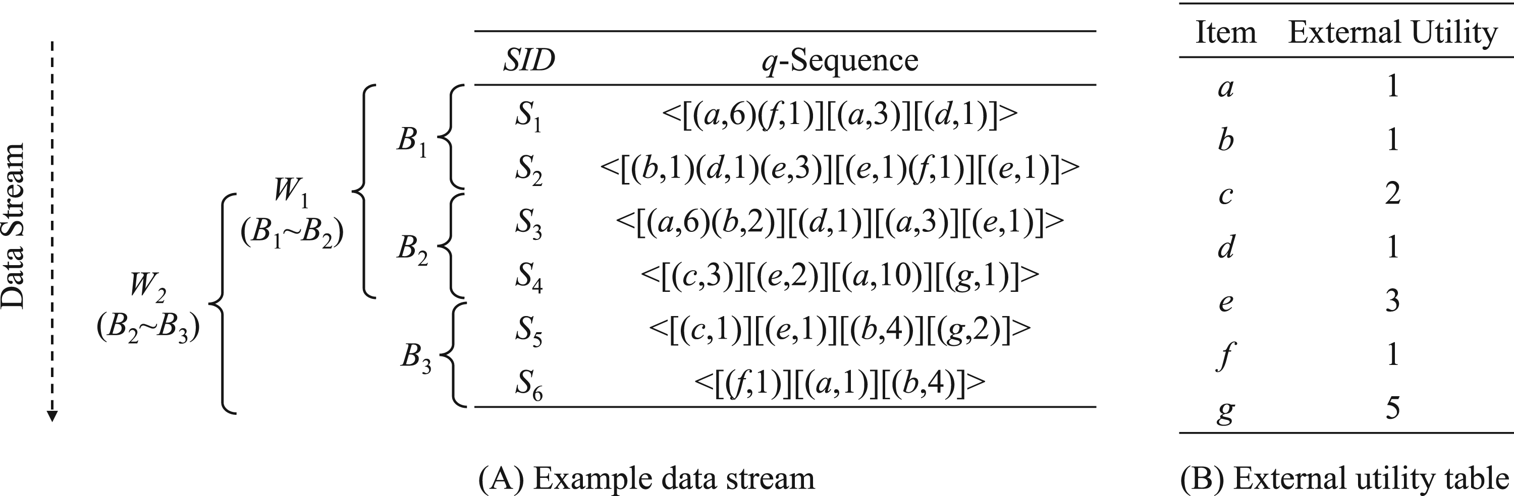
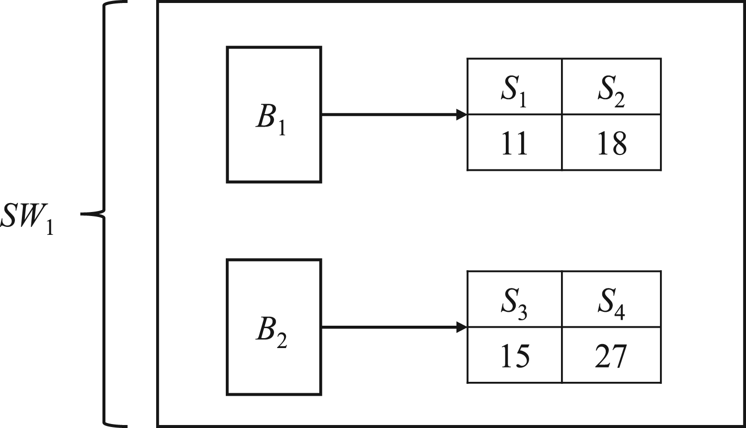
Figure 1 is an example data stream (A) and external utility table (B). Each row in Figure 1(A) represents a sequence, which consists of a sequence identifier SID and a quantized sequence. The example data stream contains a total of six sequences S_i= {S₁, S₂, S₃, S₄, S₅, S₆}, where every two sequences form a batch, resulting in a total of three batches B_j= {B₁, B₂, B₃}. Furthermore, every two batches form a sliding window, leading to a total of two sliding windows W_s= {W₁, W₂}.

Figure 1.

Example data streams and external utility table.

Definition 1

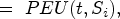
The utility of item/itemset.¹⁹ The utility value of item i in the jth itemset in sequence S is defined as $u (i, j, S) = p (i) \times q (i, j, S)$ , where p(i) is the external utility of item i and q(i,j,S) is the internal utility. The utility of the itemset in sequence S is defined as $u (I, S) = \sum_{\forall i \in I \land I \subseteq s} u (i, j, S)$ .

For example, considering the example data streams, the utility value of item a in the first itemset of sequence S₁ is denoted as u(a,1,S₁) = 6 × 1 = 6. The utility value of the first itemset [a, f] in sequence S₁ is calculated as u([a, f], S₁) = 6 × 1 + 1 × 1 = 7.

Definition 2

q-sequence utility.¹⁹ The utility value of q-sequence S_i is defined as $S U (S_{i}) = \sum_{\forall I \subseteq S_{i}} u (I, S_{i})$ .

For example, in the example data streams, the q-sequence utility value of sequence S₁ is calculated as SU(S₁) = u([a,f],S₁) + u([a],S₁) + u([d],S₁) = 6 × 1 + 1 × 1 + 3 × 1 + 1 × 1 = 11.

Definition 3

The maximum utility of sequence t.¹⁹ Given that the non-quantized sequence t may match multiple quantized sequences S, the HUSPM problem defines the utility of t in S as the maximum matching utility of t across all S. Assume that the extended position set of all non-quantized sequences t is P = (p₁, p₂, …, p_x), then the maximum utility value of the sequence t is defined as $u (t, S) = max u (t, p_{i}, S) | \forall p_{i} \in P$ .

For example, in the example data streams, the non-quantized sequence t = <[a][e]> has two matches in sequence S₃, then u(<[a][e], S₃>) = max{u(< [(a,6)][(e,1)]>), u(<[(a,3)][(e,1)]>)} = max{9,6} = 9.

Definition 4

Remaining utility.¹⁹ The remaining utility of sequence t at position p in S_i is defined as $r u (t, p, S_{i}) = \sum_{t \subseteq S_{i}} u (t / S_{i}, p)$ .

For example, in the example data streams, the remaining utility of sequence t = <[a]> at the first matching position in sequence S₁ is calculated as ru(t, 0, S₁) = u(<[(f,1)][(a, 3)][d,1]>,S₁) = 1 + 3 + 1 = 5.

Definition 5

The total utility of a batch. The total utility of a batch in the sliding window SW_k is $B U (B_{i}) = \sum_{S_{j} \subseteq B_{i}} S U (S_{j})$ .

For example, in the example data streams, the total utility of batch B₁ is calculated as BU(B₁) = SU(S₁) +SU(S₂) = 11 + 18 = 29.

Definition 6

Total utility of a window. The total utility of a sliding window SW_k is expressed as $W U (W_{k}) = \sum_{B_{i} \in W_{k}} B U (B_{i})$

For example, in the example data streams, the total utility of window SW₁ is calculated as WU(W₁) = BU(B₁) +BU(B₂) = 29 + 27 = 56.

Definition 7

Batch weighted utility of sequence t. The utility value of sequence t in batch B_i is the sum of the maximum utility values of sequence t in all S_j, defined as $B W U (t, B_{i}) = \sum_{t \subseteq S \land S \in B_{i}} u (t, S)$ .

For example, in the example data streams, the utility of sequence t = <[a]> in batch B₁ is BWU (t, B₁) = u (t, S₁) + u (t, S₂) = 6 + 0 = 6.

Definition 8

Window weighted utility of sequence t. The utility value of sequence t in window W_s is the sum of the weighted utility values of sequence t within the batch, defined as $W W U (t, W_{s}) = \sum_{t \subseteq S \land S \subset B \land B \subseteq W_{s}} B W U (t, B)$ .

For example, in the example data streams, the weighted utility of sequence t =<[a]> in window W₁ is WWU (t, W₁) = BWU (t, B₁) + BWU (t, B₂) = 6 + 16 = 22.

Definition 9

Data streams. Data streams DS = {S₁, S₂, …, S_t, …} is an ordered and infinite sequence composed of quantized sequences, where S_t (t = 1, 2, …) is generated by the t-th sequences, each containing a unique sequence identifier SID.

Definition 10

High utility sequential patterns. If the utility value of sequence t in the sliding window SW_k is not less than the minimum utility threshold (minutil), then sequence t is called high utility sequential patterns, which is defined as follows: $HUSPs \leftarrow t | W W U (t, W_{k}) \geq min u t i l$ .

For example, the utility of sequence t = <[a]> in window SW₁ is WWU (t, W₁) = 22. If minutil = 20, sequence t is called a high utility sequential pattern in SW₁.

4 Proposed algorithm

This section initiates with an introduction to the algorithm's search space and the employed pruning strategy. Subsequently, it delineates the designed data structure and outlines the steps in algorithm design. Finally, a comprehensive complexity analysis of the algorithm is provided.

4.1 Search space and pruning strategy

4.1.1 Search space

The Lexicographic Q-sequence tree (LQS-tree) structure serves as an extension of the lexicographic sequence tree,²⁶ a commonly utilized framework in HUSPM for representing the search space.^1,19 Figure 2 illustrates the structure of the LQS-tree built based on sample data streams. The root node of the LQS-tree is an empty node, and subsequent child nodes extend from their parent node. Each node within the tree signifies a candidate sequence, with all nodes organized in ascending alphabetical order within the dictionary. The adoption of the LQS tree is motivated by its effective approach to pattern growth and the recursive projection. The algorithm employs a depth-first search to recursively generate sub-sequences based on prefix sequences. Utilizing the LQS-tree helps prevent the generation of patterns not present in the window or redundant testing of the same patterns. This ensures efficiency in pattern generation and testing within the algorithm.

Figure 2.

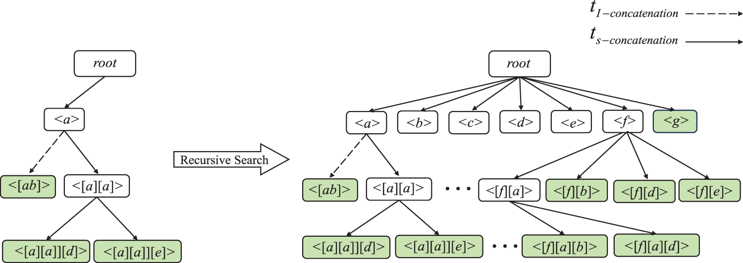
Lexicographic Q-sequence tree.

Definition 11

Concatenation operation.¹ Given a sequence t = <I₁,I₂, …, I_n> and an item to be expanded i_k, the I-Concatenation operation refers to adding the item i_k to be expanded to the sequence t in the last itemset I_n, it is recorded as $t_{I - c o n c a t e n a t i o n} \to i_{k}$ ; S-Concatenation operation refers to treating the item i_k to be expanded as a new itemset I_n + 1 and adding it after the last itemset I_n, recorded as $t_{S - c o n c a t e n a t i o n} \to i_{k}$ .

For example, in the example data streams, let's consider the sequence t = <[b]> and the item e to be expanded in S₂. The subsequence obtained after operating $t_{I - c o n c a t e n a t i o n} \to e$ on the given sequence t is $t_{1}$ =<[be]>. After operating $t_{S - c o n c a t e n a t i o n} \to e$ , we get the subsequence $t_{2}$ = <[b][e]>. It can be seen that after the operation $t_{I - c o n c a t e n a t i o n} \to i_{k}$ , the number of itemsets contained in the sequence does not change, but after the operation $t_{S - c o n c a t e n a t i o n} \to i_{k}$ , the number of itemsets contained in the sequence increases by one. Based on the above two operations, the algorithm can enumerate all possible sequences, generate candidate pattern trees, and finally mine complete high utility sequential patterns.

4.1.2 Pruning strategy

Definition 12
Sequence weighted utilization (SWU).¹ Given a sequence t, its sequence weighted utility in the current window W_s refers to the sum of the utility of all q-sequences containing t in the window. The specific definition is as follows formula (1) shows:
$S W U (t) = \sum_{t \subseteq S \land S \in W_{s}} S U (S_{i})$
(1)

For example, SWU (<a>) of sequence t =<[a]> in window W₁= SU(S₁) + SU(S₃) + SU(S₄) = 11 + 15 + 27 = 53.
Theorem 1
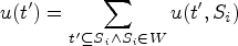
Given a quantified sequence window W and two sequences t and t’, if t’ is a superset of t, then the following relationship exists: $u (t^{'}) \leq S W U (t^{'}) \leq S W U (t)$ .
Proof
Because t’ is a superset of t, then the number of q-sequences containing t is greater than or equal to the number of q-sequences containing t’, so $S W U (t^{'}) = \sum_{t^{'} \subseteq S_{i} \land S_{i} \in W} S U (S_{i}) \leq \sum_{t \subseteq S_{i} \land S_{i} \in W} S U (S_{i}) = S W U (t)$ and because $t^{'} \subseteq S_{i}$ , S _i is the q-sequence where $t^{'}$ is located, then $u (t^{'}) \leq S U (S_{i})$ , so $u (t^{'}) \leq \sum_{t^{'} \subseteq S_{i} \land S_{i} \in W} S U (S_{i}) = S W U (t^{'})$ .

Pruning strategy 1: Given a minimum utility threshold minutil and a sequence t, if SWU(t) is less than or equal to minutil, then stop searching for t and its superset, because t and its superset are all unpromining candidate sequences.
Definition 13
Prefix extension utility (PEU).¹⁹ Given a sequence t, its prefix extension utility at position p is defined as follows:
$P E U (t, p, S_{i}) = {\begin{matrix} u (t, p, S_{i}) + r u (t, p, S_{i}), & i f r u (t, p, S_{i}) > 0 \\ 0, & o t h e r w i s e \end{matrix}$
(2)

Among them, u(t,p,S_i) refers to the utility of sequence t at position p, and ru(t,p,S_i) refers to the remaining utility of sequence t at position p (excluding the element at position p).

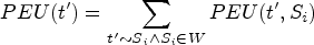
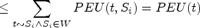
The PEU of sequence t in q-sequence S_i is defined as:
$P E U (t, S_{i}) = max {P E U (t, p, S_{i}) | \forall e x t e n s i o n p o s i t i o n p o f t i n S_{i}}$
(3)
Note that the PEU of sequence t in window W is defined as:
$P E U (t) = \sum_{t \subseteq S_{i} \land S_{i} \in W} P E U (t, S_{i})$
(4)
For example, in window W₁, the sequence t = <[a]> has two matches in S₁, namely <[(a,6)]> and <[(a,3)]>. The utilities are 6 and 3 respectively; the remaining utilities are 5 and 1 respectively, then PEU(t,S₁) = max{6 + 5,3 + 1} = 11. PEU(t) of sequence t in database W₁= PEU(t,S₁) + PEU(t,S₃) + PEU(t,S₄) = 11 + 15 + 15 = 41.
Theorem 2
Given a quantized sequence window W and two sequences t and t’, if t’ is a superset of t, then the following relationship exists: $u (t^{'}) \leq P E U (t^{'}) \leq P E U (t)$ .
Proof
First prove the first half of the equation, because
$\begin{aligned} u (t^{'}, S_{i}) & = max {u (t^{'}, S_{i})} \end{aligned}$

$\begin{aligned} \leq max {u (t^{'}, S_{i}) + r u (t^{'}, S_{i})} \end{aligned}$

$\begin{aligned} = P E U (t, S_{i}), \end{aligned}$
so
$\begin{aligned} u (t^{'}) & = \sum_{t^{'} \subseteq S_{i} \land S_{i} \in W} u (t^{'}, S_{i}) \end{aligned}$

$\begin{aligned} \leq \sum_{t^{'} \sim S_{i} \land S_{i} \in W} P E U (t^{'}, S_{i}) \end{aligned}$

$\begin{aligned} = P E U (t^{'}) \end{aligned}$

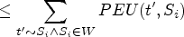
Let's prove the second half of the equation. Because t’ is a superset of t, so $u (t^{'}, S_{i}) + r u (t^{'}, S_{i}) \leq u (t, S_{i}) + r u (t, S_{i})$ , we can get
$\begin{aligned} P E U (t^{'}, S_{i}) & = max u (t^{'}, S_{i}) + r u (t^{'}, S_{i}) \end{aligned}$

$\begin{aligned} \leq max u (t, S_{i}) + r u (t, S_{i}) = P E U (t, S_{i}) \end{aligned}$

$\begin{aligned} P E U (t^{'}) & = \sum_{t^{'} \sim S_{i} \land S_{i} \in W} P E U (t^{'}, S_{i}) \end{aligned}$

$\begin{aligned} \leq \sum_{t \sim S_{i} \land S_{i} \in W} P E U (t, S_{i}) = P E U (t) \end{aligned}$
Therefore, for all t and t’, there is the following relationship: $u (t^{'}) \leq P E U (t^{'}) \leq P E U (t)$ .

Pruning Strategy 2: Given a minimum utility threshold minutil and a sequence t, if PEU(t) is less than or equal to minutil, then terminate the search for t and its supersets. This is because both t and its supersets are considered unpromising candidate sequences.
Definition 14
Compact Sequence Utility (CSU) Assume that sequence t has i matches in the quantized sequence S of window W, and their matching positions are δ₁, δ₂, …, δ_i, where δ₁<δ₂< … <δ_i, given by t the subsequence generated by performing I-Concatenation or S-Concatenation operation on item k is t’, and the minimum position of item k to be expanded in S (i.e., the first matching position) is p₁ (δ_i< p₁), then CSU is defined as in formula (5), where u(t,δ,s) = max{u(t,δ_i,s)} refers to the maximum utility value of prefix t in S.
$C S U (t^{'}, S) = {\begin{matrix} u (t^{'}, p_{1}, S) + r u (t^{'}, p_{1}, S), & i f l e n g t h = 1 \\ u (t, δ, S) + u (k, p_{1}, S) + r u (k, p_{1}, S), & i f length \geq 2 \end{matrix}$
(5)

Note that the CSU of sequence t’ in window W is defined as:
$C S U (t^{'}, W) = \sum_{\forall t \subseteq S_{i} \land \forall S_{i} \in W} C S U (t^{'}, S_{i})$
For example, given a 1-sequence t = <[a]>, in S₁ of the example data streams, its CSU(t,S₁) = u(a,1,S₁) +ru(a,1,S₁) = 6 + 5 = 11. For another example, in S₃ of the example data streams, given a sequence t = <[ab]>, the item to be expanded is a, that is, t’ = <[ab][a]>, and its CSU(t’,S₃) = u(<[ab]>,S₃) + u(a,S₃) + ru(a,S₃) = 8 + 3 + 3 = 14.
Theorem 3
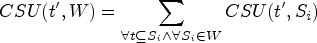
Given a quantified sequence window W and two sequences t and t’, if t’ is a superset of t, then the following relationship exists: $u (t^{'}, S) \leq C S U (t, S)$ .
Proof
First, prove that when the length of is 1. All sequences are single-item sequences. u(t’,S) is the maximum value at each extended position p_j in the q-sequence S. When u(t’,S) = u(t’,p₁,S), u(t’,S) $\leq$ u(t’,p₁,S) + ru(t’,p₁,S) = CSU(t’,S); when u(t’,S) ≠ u(t’,p₁,S), so u(t’,S) $\leq$ u(t’,p₁,S) + ru(t’,p₁,S) = CSU(t’,S). Prove again, when the length of t’ is greater than or equal to 2. When δ_i< p₁, u(t,δ,S) = max{u(t, δ_i, S)} ensures that the utility of the prefix item t is the maximum, that is, u(t,S) $\leq$ max{u(t,δ_i,S)}. And u(k,p₁,S) + ru(k,p₁,S) ensures that all the items to be extended k and the suffixes of k are less than the sum of the utility and the remaining utility at the first position, that is, u(t'_S|t) $\leq$ u(k,p₁,S) + ru(k,p₁,S), where u(t'_S|t) refers to the sum of the utility of the extended item that does not include the prefix t and all its suffixes, then u(t’,S) $\leq$ u(t,S) + u(k,p₁,S) + ru(k,p₁,S).

For example, in S₂ of the example data stream, the item to be expanded for the sequence t = <[b]> is e, and the subsequence formed by S-Concatenation of the sequence t is t’ = <[b][e]>. Among them, the first position of the item e to be expanded is 3. When δ < 6, the maximum utility value of the prefix [b] is u(<[(b,1)]>) = 1. Because the length of the sequence t’ is greater than or equal to 2, then CSU(<[b][e]>, S₂) = u(<[(b,1)]>) + u(e,S₂) + ru(e,S₂) = 1 + 3 + 4 = 8, guaranteeing the most compact upper bound.

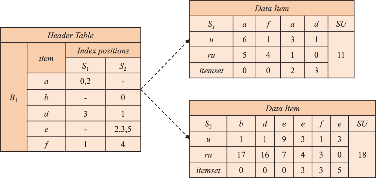
Pruning strategy 3: Given a minimum utility threshold minutil and a sequence t, if CSU(t) is less than or equal to minutil, then stop searching for t and its superset, because t and its superset are all unpromising candidate sequences.
4.2 Dynamic utility index table

The paper introduces a data structure called the dynamic utility index table (DUI-table). This structure is constructed or updated after scanning the current window and encompasses all batches within the window. As the window slides, the oldest batches are removed, and new batches are added. Figure 3 illustrates the information of the two batches contained in the initial window.

Figure 3.

DUI-table structure within the first window.

The DUI-table structure is utilized for storing information about sequences within the sliding window W_s, including the batch they belong to, index positions, and utility information. Each DUI-table structure consists of two parts: the header table and data items. The header table stores the current batch number B_i, non-repeated items contained in the batch, and their respective positions in the sequences. The data items are used to store information about the current sequence, sequence identifier (SID), utility u, remaining utility ru, and the starting position in the itemset (same position indicates within the same itemset). The structure of the dynamic utility index table for the first batch in the initial window is depicted in Figure 4.

Figure 4.

Dynamic utility index table structure for B₁.

The DUI-table structure provides an equivalent projection window to the original window with significantly reduced space requirements. By scanning the initial DUI-table structure and constructing new sequence DUI-table structures based on the currently obtained prefix sequences, it only retains the corresponding suffix sets. Therefore, the total number of sequences in the DUI-table is always less than or equal to the size of the original window data. Figure 5 illustrates the projection DUI-table based on the prefix <[a]> for the first batch. The suffix set in S₁, based on <[a]>, includes elements <[f],[a],[d]>. The DUI-table retains information only for the corresponding suffix set, while S₂ does not contain the element <[a]>, resulting in an empty storage for S₂. The DUI-table, following a pattern-growth approach, constructs a projection window for each sequence that appears in the data streams. It does not construct sequences outside the window. In other words, during each projection operation, the DUI-table is first constructed, then scanned, and subsequently used to build the next DUI-table structure based on its prefix. As the sequence pattern grows, and S_i containing the sequence becomes less frequent, the size of the projected DUI-table gradually decreases. This results in a reduction in the generated new sequences, leading to an acceleration in the search speed of the algorithm.

Figure 5.

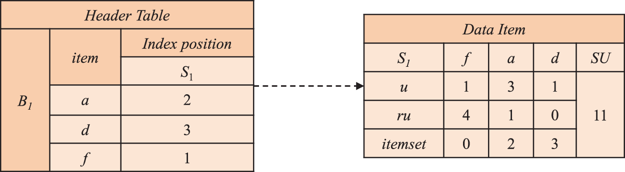
Projected DUI-table based on prefix <[a]> within batch B₁.

Based on the designed DUI-table structure in this paper, the dynamic utility index table possesses the following characteristics: (1) Projection mechanism. DUI-table is based on a projection mechanism using prefixes. It recursively partitions the DUI-table structure without the need to construct a projected sub-window. This approach forms a divide-and-conquer mining framework. The information about sequences obtained through the prefix projection mechanism is accurate and does not generate sequences outside the window. (2) Compact structure. The DUI-table structure comprises a header table and data items. The header table stores non-repeating items in the sequence along with their index positions, while data items store the items, utility values, remaining utility, itemset positions, and q-sequence utility (SU) in the sequence. It requires only a negligible amount of memory to construct, enabling the handling of a substantial number of sequences within limited memory resources. (3) Efficiency. The DUI-table structure accelerates sequence generation, enhances the computation speed of subsequence utility values and upper bounds. Furthermore, it records the position information of extension items, eliminating the need to traverse the entire sequence to find all extension points. This capability facilitates the identification of candidate sequences, enabling the recognition of all high utility sequential patterns within a finite time frame.

4.3 Algorithm description

Based on the DUI-table structure and the pruning strategies mentioned above, this paper proposes an algorithm, named HUSP_DS, for mining high utility sequential patterns over data streams based on the sliding window model. The overall mining process of the algorithm is illustrated in Figure 6.

Figure 6.

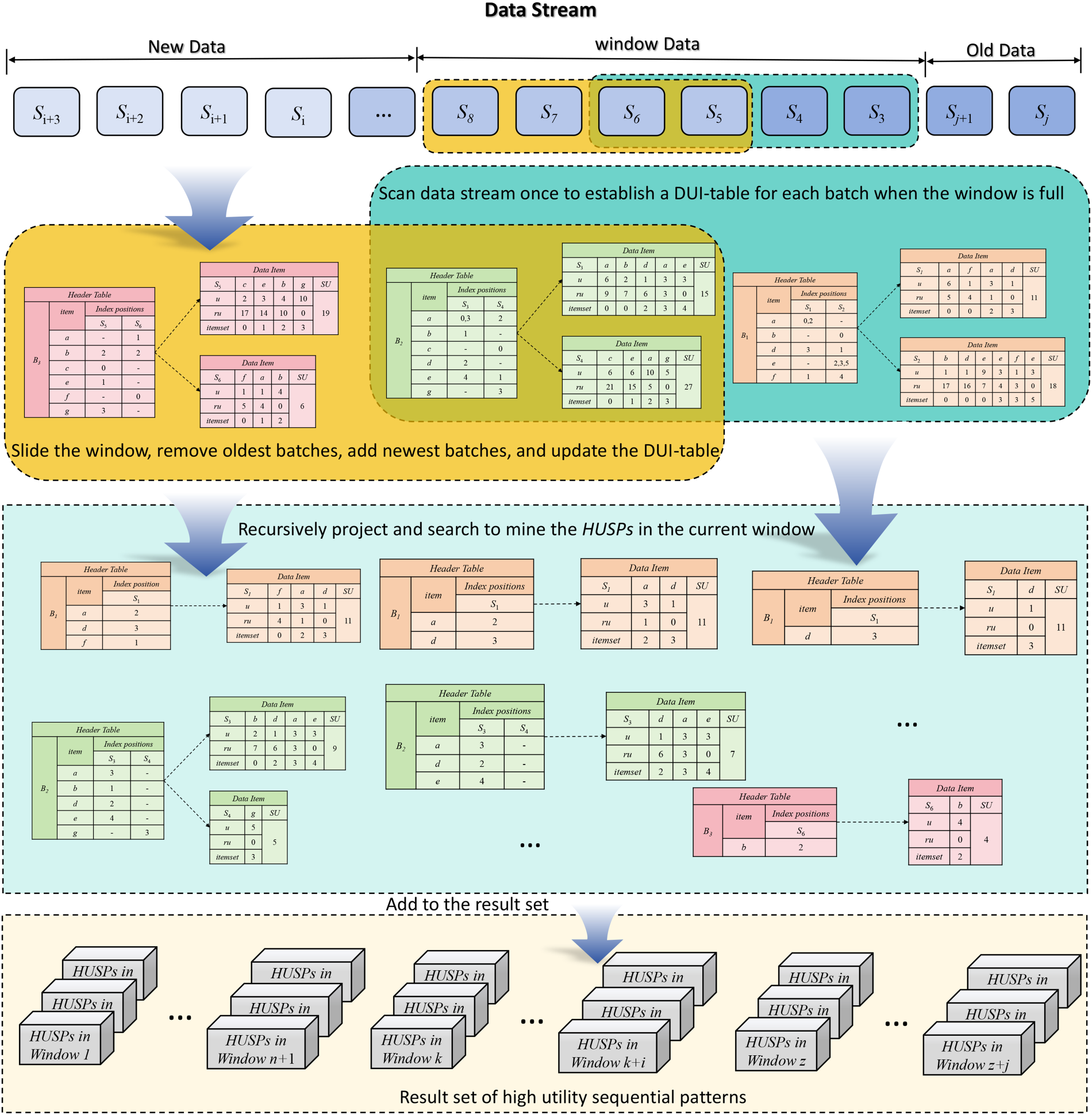
General framework of the algorithm.

The algorithm can be divided into three modules: initialization, mining, and search. Algorithm 1 represents the main program of the proposed algorithm. The algorithm utilizes a sliding window model to process data streams, where the data from the first window are added all at once upon arrival, while subsequent windows require the removal of old batches and addition of new batches. Therefore, different processing methods are employed for the first window. Firstly, the algorithm scans the data stream to determine if it is the first window. If it is, the newly arrived sequences from the data stream are added to the current batch (lines 1–5). Subsequently, the algorithm checks if the batch limit in the current window is reached. If the number of batches in the window equals the user-defined batch size, the new batch is added to the window (lines 6–8). When the window is full, the mining algorithm is invoked to process the first window (lines 9–12).

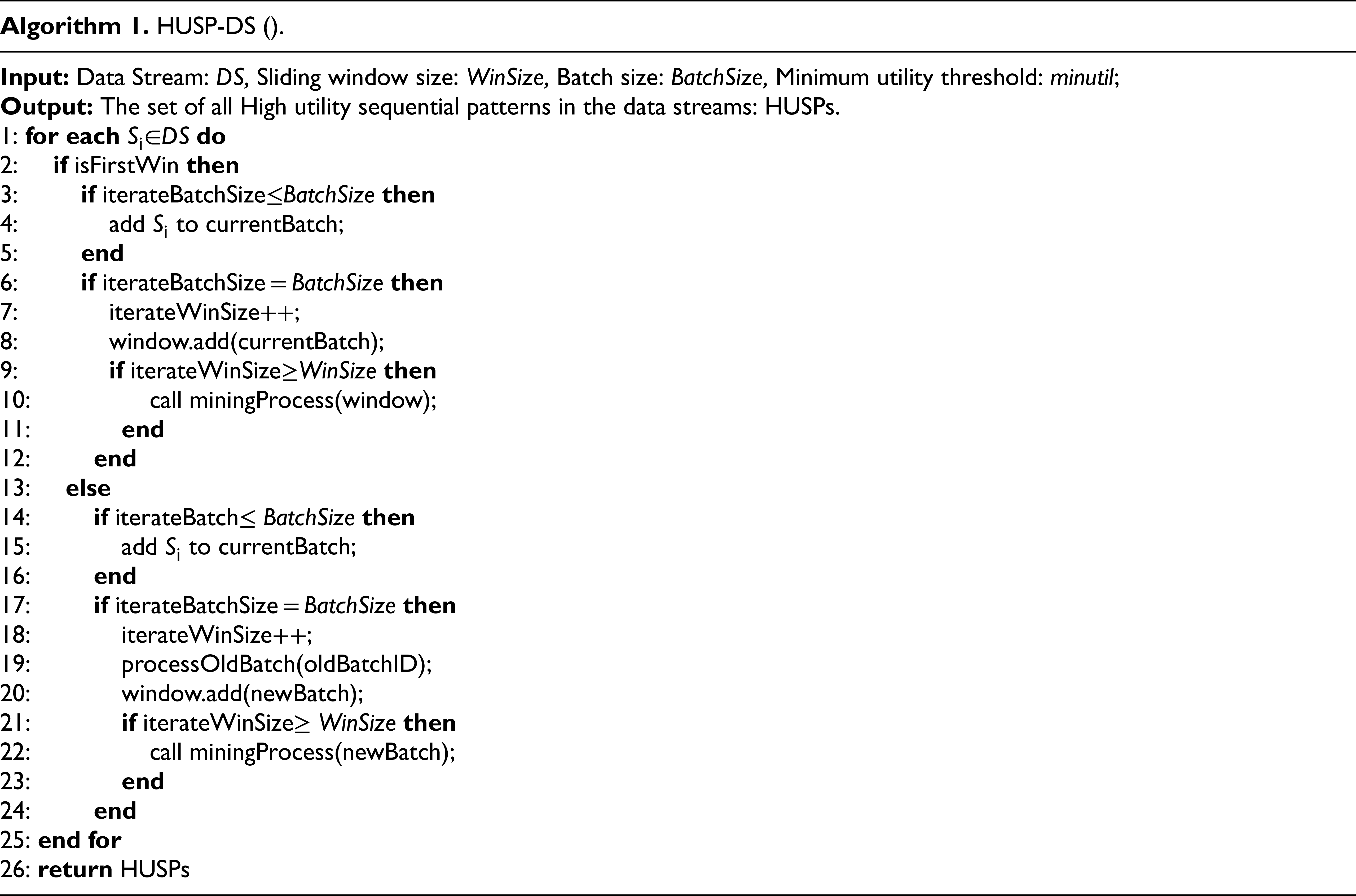
Secondly, if the current window is not the first one, the algorithm adds new batches until the window size meets the specified size. Then, it slides the window, simultaneously processing the old and new batches (lines 13–26).

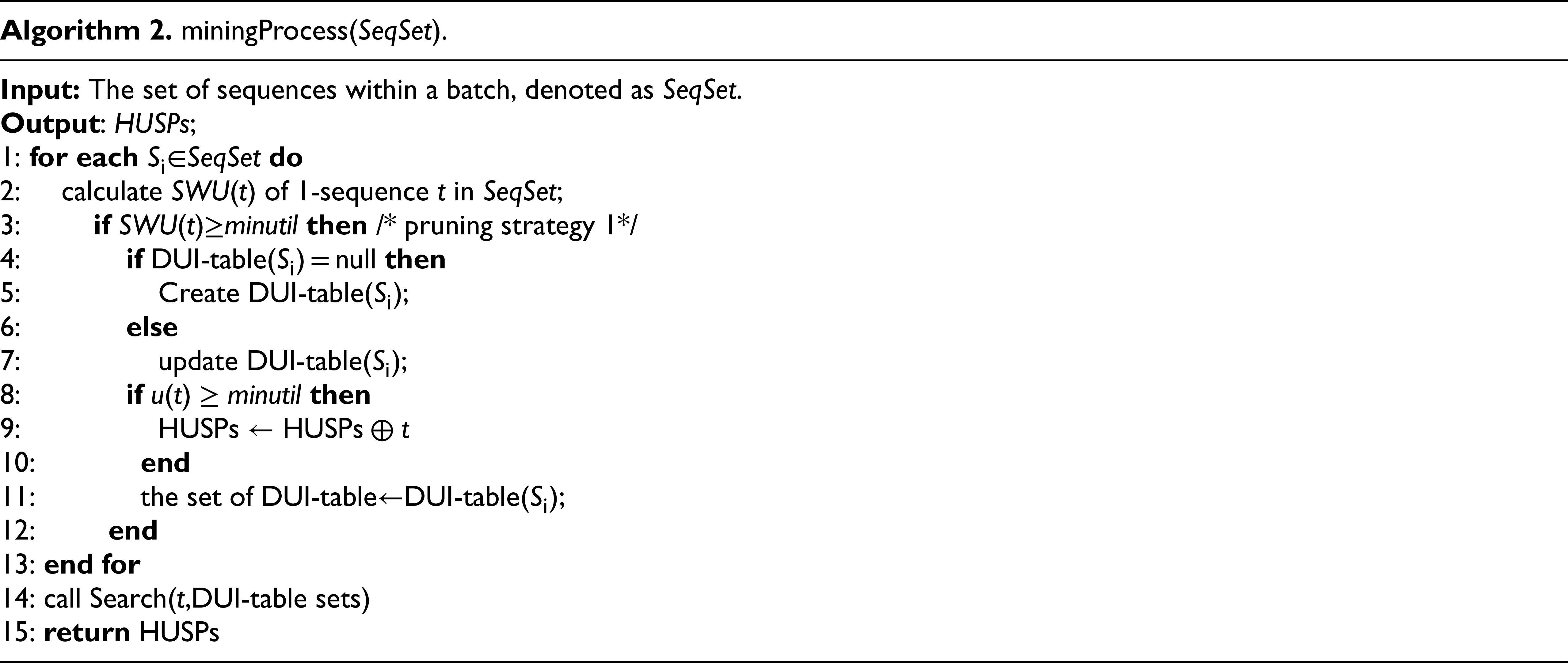
Algorithm 2 initializes and updates the DUI-table, mines all high-utility 1-sequence sets, and calls Algorithm 3 for search and mining when the window is full or the data stream stops. Algorithm 2 scans the sequence set SeqSet within the window and evaluates each sequence in the batch, calculating the sequence weighted utility for all 1-sequences. If the sequence weighted utility is not less than the minimum utility threshold and the sequence's DUI-table is empty, a DUI-table is created for that sequence; otherwise, the sequence's DUI-table is updated (lines 1–7). Then, the actual utility values for all 1-sequences are calculated, and sequences with utility values greater than or equal to the predefined threshold are added to the pattern result set HUSPs according to definition 10 (lines 8–10). Each sequence's DUI-table is added to the DUI-table set after creation or updating, and a depth-first search is performed by calling the recursive search Algorithm 3 based on the prefix sequences (lines 11–15).

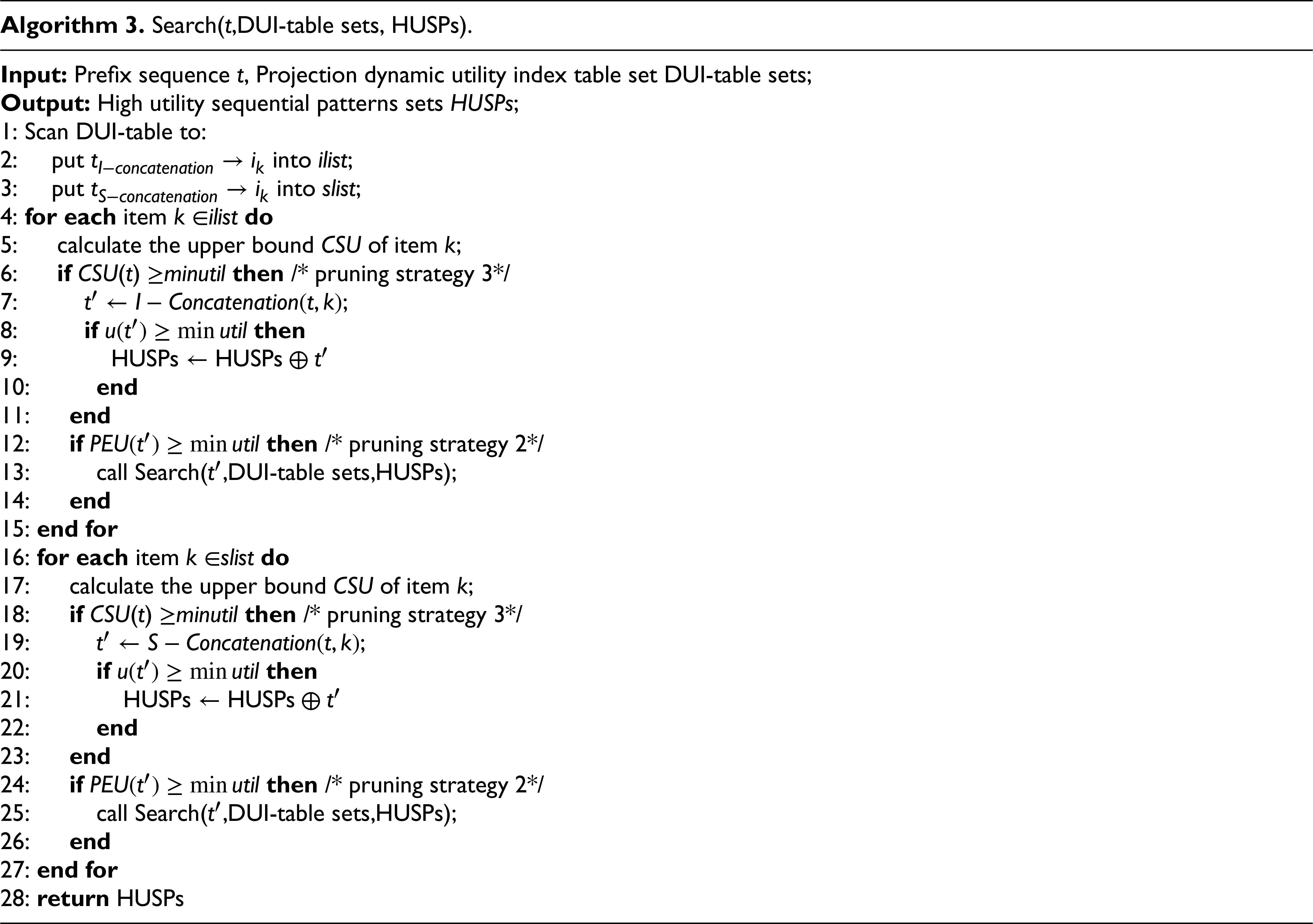
To determine whether the newly generated sequence is a candidate sequence and a high utility sequential pattern, Algorithm 3 scans the DUI-table to obtain information about the new sequence. As the search space of the algorithm is arranged in lexicographic order based on the alphabetical sequence of the lexicographic q-sequence tree, the algorithm conducts a depth-first search, recursively moving downward based on prefix sequences until all high utility sequences are identified. Firstly, the algorithm scans the DUI-table and adds candidate sequences from $t_{I - c o n c a t e n a t i o n} \to i_{k}$ operations to the ilist and those from $t_{S - c o n c a t e n a t i o n} \to i_{k}$ operations to the slist (lines 1–3). Subsequently, the algorithm calculates the compact sequence utility (CSU) upper bound for the extension item k in ilist. It employs pruning strategy 3 to prune unpromising candidate sequences. If the CSU value of a candidate sequence is not less than the user-specified minimum utility threshold, the algorithm performs extension operations based on that sequence, generates a new sequence t’, calculates its utility value, determines whether it is a high utility sequential pattern, and adds it to the result set (lines 4–11). The algorithm then recursively calls the search algorithm for mining, using the new sequence t’ as the prefix, until all high utility sequential patterns are identified (lines 12–15). For the sequences in slist, the algorithm applies similar operations to those in ilist (lines 16–28).

4.4 Algorithm examples

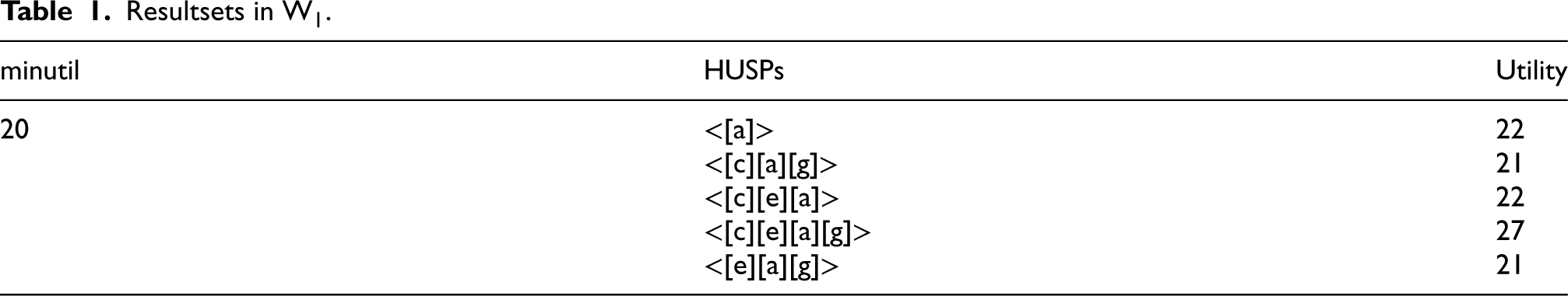
To better understand the algorithm proposed in this paper, this section uses an example to describe the working principles of the algorithm. Consider the example data stream shown in Figure 1, where the window size is 2B (i.e., each window contains two batches), the batch size is 2 (i.e., each batch contains two sequences), and the minimum utility threshold is set to 20. Figure 7 illustrates the DUI-table structure of the example data streams, including two windows and three batches.

Figure 7.

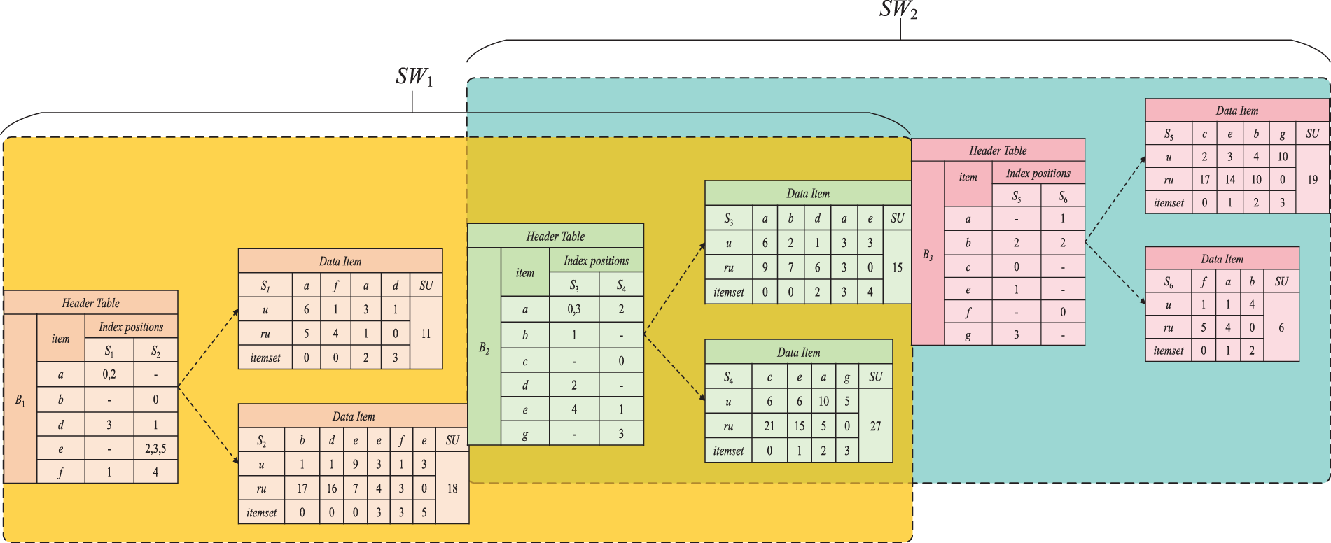
DUI-table structure in the example data streams.

Step 1: Initialization. The algorithm initializes the window size and batch size. As the data stream arrives, it reads the data of the specified size batch and inserts it into the window. When the window is full, the algorithm calls the mining function “miningProcess()” for mining, as shown in Algorithm 1.

Step 2: Build DUI-table. For each sequence read, the DUI-table structure is established in batches. The header table stores the elements of non-repeating items and their index positions in each sequence in alphabetical order, and the data items store the current sequence and utility information. After the algorithm has established the DUI-table for all batches in the current window, Algorithm 2 starts to calculate the SWU of 1-sequence t and determine whether all single-item sequences are high utility sequential patterns. If they are high utility sequential patterns, they are added to the result set.

For example, in Figure 1, batch B₁ contains two sequences S₁ and S₂, in which all non-repeating items include a, b, d, e, and f. Therefore, the header table of DUI-table stores a, b, d, e, and f as well as their index positions in sequences S₁ and S₂, and the data items store sequence elements, utility, remaining utility, and the starting position of the itemset, as shown in Algorithm 2. After calculation, according to definition 10, the utility value of the single-item sequence <[a]> in W₁ can be calculated to be 22, and its utility is greater than the minimum utility threshold of 20. Therefore, <[a]> is a high utility sequence.

Step 3: Recursive projection and search. Next, the algorithm then calculates the PEU and CSU values for the prefix sequence <[a]> and adds it to the candidate sequence if it exceeds the minimum utility threshold. After that, based on the prefix <[a]>, the algorithm attempts extensions. Assuming the extension item is ‘a’, the algorithm first performs the $t_{I - c o n c a t e n a t i o n} \to a$ operation in a depth-first manner. Scanning the projected DUI-table reveals that the sequence <[a, a]> is not present in the current data, so the search is terminated. The algorithm then proceeds with the $t_{S - c o n c a t e n a t i o n} \to a$ operation, scanning the projected DUI-table and calculating the utility value for the sequence <[a][a]> in the current window, resulting in a utility value of 18. This makes the sequence t = <[a][a]> a low utility sequence. The depth-first search for the prefix <[a][a]> is terminated. This process continues, recursively searching for all high utility sequences in the current window and adding them to the result set.

Step 4: The window slides. The result set of high utility sequential patterns in the sliding window W₁ is shown in Table 1. Subsequently, the algorithm deletes the oldest batch B₁ from W₁, reads the new batch B₃, slides the window forward, establishes a DUI-table for the new batch, deletes the DUI-table of the old batch, adds the DUI-table of the new batch to the DUI-table set, and performs a recursive search process similar to that in W₁ again until the data stream is empty and the algorithm terminates.

Table 1.

Resultsets in W₁.

minutil	HUSPs	Utility
20	<[a]>	22
	<[c][a][g]>	21
	<[c][e][a]>	22
	<[c][e][a][g]>	27
	<[e][a][g]>	21

4.5 Complexity analysis

The time consumption of the HUSP_DS algorithm mainly includes: ① establishment and update of DUI-table; ② recursive expansion search process. First, assume that the number of sequences contained in the current window is n_w, the average length of the sequence is S_avg, and the number of sequences in the new batch contained in the current window is n_b. For the first window, the algorithm needs to traverse all batches and sequences and create a DUI-table for each sequence, so the time required for the first window is O(n_w× S_avg). For other windows, the algorithm only needs to establish a DUI-table for the sequences in the new batch, and the time complexity required for the other windows is O(n_b× S_avg). Therefore, the time complexity required by the algorithm in the DUI-table establishment and maintenance phase is O((n_w+ n_b)×S_avg). Secondly, when the window is full, the algorithm recursively calls the Search() operation to perform depth-first search. The number of calls to the Search() operation is proportional to the number of prefixes t. In the worst case, if none of the prefixes are pruned, then the algorithm the time required is O(2^m − 1).

The space consumption of the algorithm is mainly the establishment and maintenance of DUI-table. Assume that the header table of each batch contains n_t different items, each batch contains n_b sequences, and the average length of each sequence is S_avg. The space complexity required to create the DUI-table header table is O(n_t+ S_avg), and the space complexity required to create the data items is O(n_b× S_avg). Then the total space complexity of the algorithm is O(n_t+ S_avg+ n_b× S_avg).

In short, in the worst case, the total time complexity of the algorithm is O((n_w+ n_b)×S_avg+ 2^m − 1), and the total space complexity of the algorithm is O(n_t+ S_avg+ n_b× S_avg). It is worth noting that as the sequence length increases, the number of sequences contained in the database decreases, the projected dynamic utility index table decreases, the number of candidate sequences and the number of items to be expanded also decreases accordingly, and the running time of the algorithm will also be accelerated. Therefore, the actual running time and memory consumption required by the algorithm may be less.

5 Experiments

To assess the effectiveness of the HUSP_DS algorithm, this section conducts a comprehensive set of experiments to evaluate the algorithm's efficiency. The experiments encompass its performance in three scenarios: 1) the impact of threshold size on algorithm performance; 2) the influence of window size and batch size on algorithm performance; 3) the effect of dataset size on algorithm performance (scalability testing).

5.1 Experimental environment and datasets

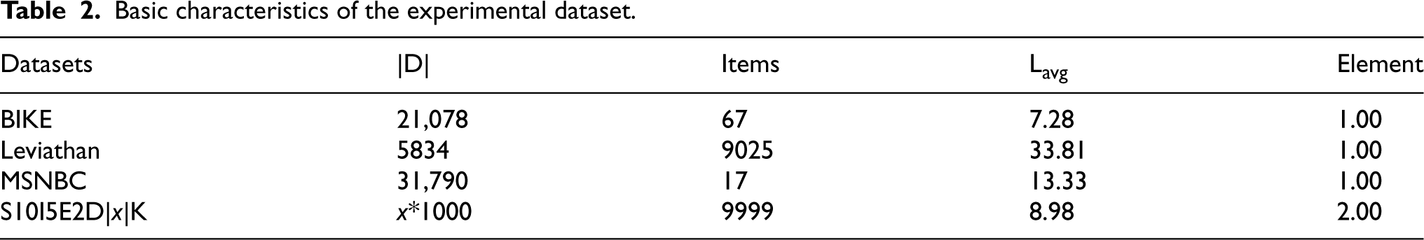
The experiments involve comparing the HUSP_DS algorithm with state-of-the-art algorithms. Since ProUM is designed for static data, it is modified to ProUM_DS to handle data streams. To test the effectiveness of pruning strategies, a comparison is made between HUSP_DS, utilizing the CSU-based pruning strategy, and HUSP_DS*, which does not use the CSU-based pruning strategy. All algorithms are implemented in Java, with the JDK version being 1.8.0_40. The experimental environment consists of an Intel(R) Xeon(R) Gold 6154 CPU running at 3.00 GHz, with 256GB of RAM, and the operating system is Ubuntu 16.04.6 LTS x86_64. Table 2 presents the datasets used in the experiments, where |D| indicates the total number of sequences in the database, Items represents the number of distinct items in the database, L_avg denotes the average length of sequences in the database, and Element indicates the average number of items in each itemset.

Table 2.
Basic characteristics of the experimental dataset.

Datasets |D| Items L_avg Element

BIKE 21,078 67 7.28 1.00

Leviathan 5834 9025 33.81 1.00

MSNBC 31,790 17 13.33 1.00

S10I5E2D|x|K x*1000 9999 8.98 2.00

Datasets	\|D\|	Items	L_avg	Element
BIKE	21,078	67	7.28	1.00
Leviathan	5834	9025	33.81	1.00
MSNBC	31,790	17	13.33	1.00
S10I5E2D\|x\|K	x*1000	9999	8.98	2.00

BIKE: Contains sequences representing the parking locations of shared bicycles in a city. Each item represents a bicycle-sharing station, and each sequence illustrates the varying positions where bicycles are parked over time. The dataset is sourced from Kaggle (https://www.kaggle.com/cityofLA/los-angeles-metro-bike-share-trip-data).

Leviathan: Derived from the novel “Leviathan” by Thomas Hobbes, this textual sequence dataset uses each word as an item. The dataset can be obtained from the website (https://www.philippe-fournier-viger.com/spmf/index.php?link=datasets.php#r3).

MSNBC: A clickstream dataset from the msnbc.com website, where user page visits are categorized by URL and recorded chronologically. The dataset is transformed from the original data in the UCI Data Repository, removing the shortest sequences and retaining 31,790 sequences. It can be found on the website (https://archive.ics.uci.edu/).

Additionally, to assess the algorithm's performance on datasets of varying sizes, a synthetic large dataset S10I5E2DD|x|K is generated using the IBM synthetic data set generator (http://www.Almaden.ibm.com/cs/quest/syndata.html). The parameter x denotes the number of sequences in the database, ranging from 100 K to 500 K.

5.2 Experimental results under different thresholds

The setting of the minimum utility threshold has a significant impact on algorithm performance. In this section, the influence of different minimum utility threshold sizes on algorithm runtime, memory consumption, and the number of generated candidate sequences is observed. Runtime is defined as the total time, including CPU runtime and disk I/O time, spent on reading input data, discovering high utility sequential patterns, and writing the results to the output file. Memory consumption is defined as the peak memory consumption throughout the entire mining process. The number of candidate sequences is defined as all sequence patterns processed during the algorithm's mining process.

Firstly, the impact of different threshold sizes on algorithm runtime is analyzed. In Figure 8, the runtime of all algorithms is inversely proportional to the threshold size. As the threshold increases, pruning strategies remove a significant number of candidate sequences, resulting in less runtime. The rate of runtime decrease varies depending on the search and pruning strategies employed by each algorithm. On the BIKE dataset, with a fixed window size of 2B and batch size of 10 K, it is evident that the proposed algorithms, with or without the CSU-based pruning strategy, are 3 to 4 orders of magnitude faster than the ProUM_DS algorithm. The ProUM algorithm requires recursive partitioning of utility arrays, and with lower thresholds, it needs to construct a massive number of projected utility arrays, leading to a rapid increase in runtime. Additionally, it is noteworthy that there is little difference in runtime between HUSP_DS and HUSP_DS*, as the BIKE dataset contains a large number of sequences, a small number of different items, and many short sequences. This makes short sequences more likely to become high utility sequential patterns, resulting in a small difference in runtime when using or not using the CSU-based pruning strategy. For the Leviathan dataset, with a window size of 2B and a batch size of 1 K, when the threshold is set low, the runtime of all three algorithms increases linearly. When the threshold is set high, the runtime of HUSP_DS and HUSP_DS* tends to stabilize with a small variation, while the ProUM_DS algorithm still exhibits a significant variation. When the minimum utility threshold changes from 4000 to 5000, the ProUM_DS runtime decreases by 36%, while the HUSP_DS runtime only decreases by 25%. This indicates that the ProUM_DS algorithm is highly sensitive to the threshold setting, as can also be observed from the MSNBC dataset. When the window size for MSNBC is set to 4B, the batch size is set to 4 K, and the threshold increases from 200 K to 240 K, HUSP_DS and HUSP_DS* algorithms show a stable trend, with the runtime difference between the minimum and maximum thresholds not exceeding 25%.

Figure 8.

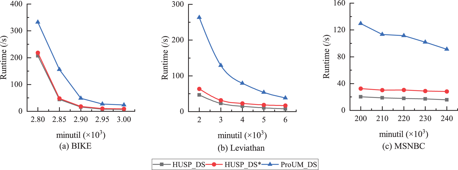
Comparison of runtime at different thresholds.

Next, the memory consumption of the algorithms is compared under different threshold values. As shown in Figure 9, in terms of memory consumption, the increase in the threshold leads to a reduction in the number of sequences in the result set, resulting in a continuous decrease in algorithm memory consumption. On the BIKE dataset, when the threshold is set to 2900, the memory consumption of HUSP_DS, HUSP_DS*, and ProUM_DS is 2294.26MB, 3113.49MB, and 2859.68MB, respectively. When the threshold is set to 2950, the average memory consumption of HUSP_DS, HUSP_DS*, and ProUM_DS decreases by about 32%, 34%, and 12%, respectively. Among them, the memory occupancy of ProUM_DS decreases most slowly, while HUSP_DS* decreases most rapidly. This is because HUSP_DS* does not use the CSU-based pruning strategy and generates more candidate sequences. On the Leviathan and MSNBC datasets, the memory consumption of the ProUM_DS algorithm is much higher than that of the HUSP_DS algorithm. As the threshold decreases, the memory consumption of the HUSP_DS algorithm remains relatively stable, while the memory consumption of the ProUM_DS algorithm increases significantly. Overall, these results fully demonstrate that the proposed algorithm outperforms state-of-the-art algorithms in terms of runtime and memory consumption, with a general improvement of 3 to 4 times in runtime and 1.4 times increase in memory consumption.

Figure 9.

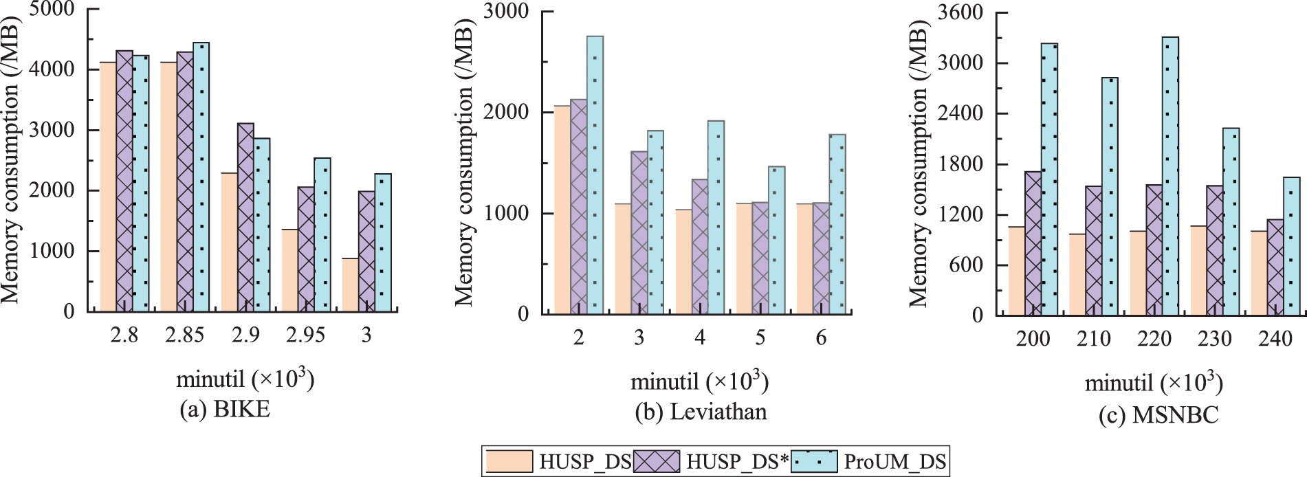
Comparison of memory consumption at different thresholds.

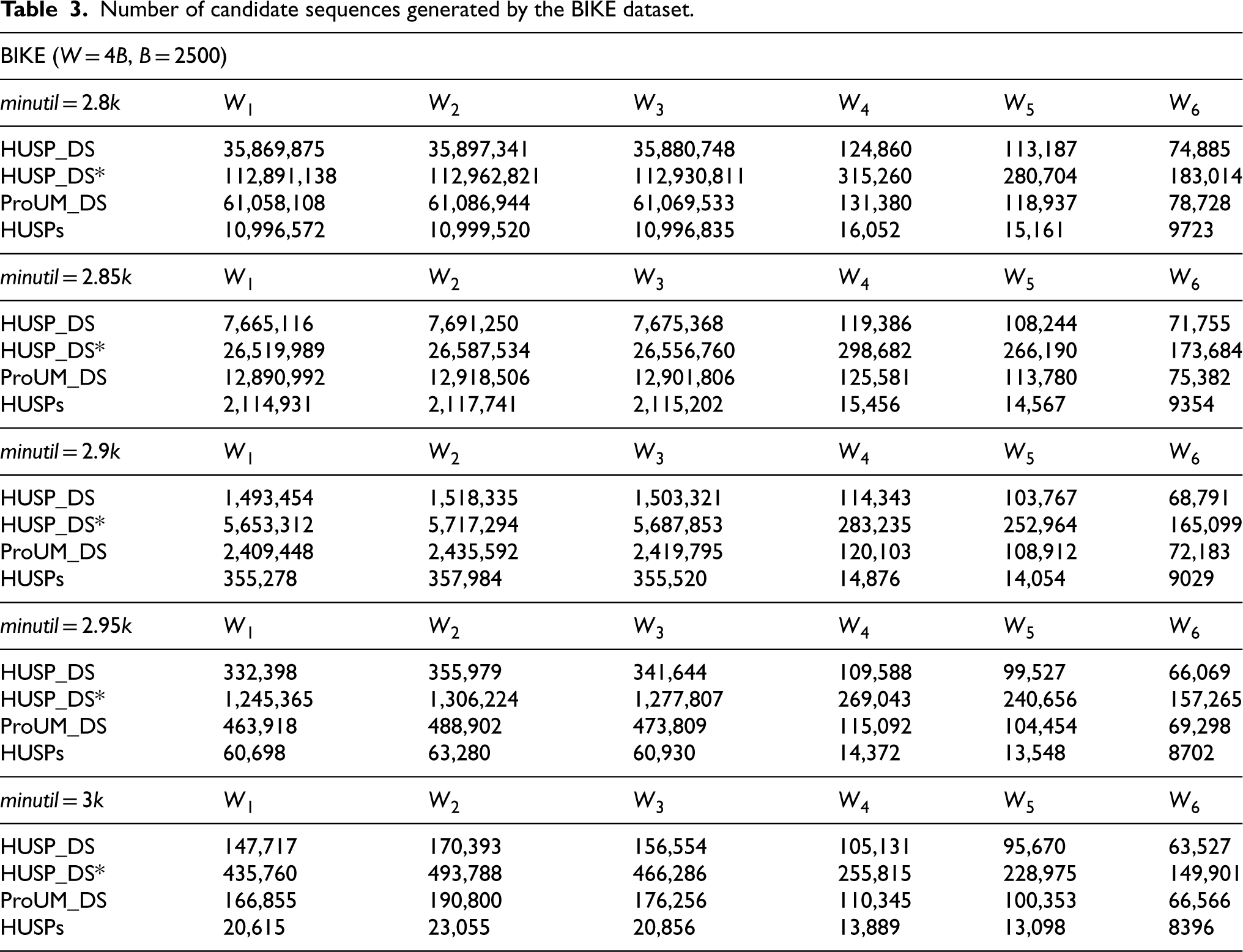
Table 3 shows the number of candidate sequences generated by each window sliding during the mining process of the BIKE dataset. The number of candidate sequences is closely related to the performance of the algorithm because once identified as candidate sequences, their actual utility values need to be calculated to determine if they are high utility sequential patterns. It should be noted that the number of patterns mined by the three algorithms is consistent. On this dataset, the window size is fixed at 4B, batch size at 2500, and the threshold is dynamically adjusted from 2.8k to 3k. Overall, the number of candidate sequences generated by the three algorithms increases with the threshold. When minutil = 2800, HUSP_DS* generates the most candidate sequences, with 2–3 times more than the ProUM_DS algorithm and 3–4 times more than the HUSP_DS algorithm. From the graph, it can be seen that when minutil = 3000, the HUSP_DS algorithm generates the fewest candidate sequences in the first window, while the HUSP_DS* algorithm generates the most, with 2.4 times more than the former. The experimental data in Table 3 shows that the HUSP_DS algorithm generates the fewest candidate sequences during the mining process.

Table 3.

Number of candidate sequences generated by the BIKE dataset.

BIKE (W = 4B, B = 2500)
minutil = 2.8k	W ₁	W ₂	W ₃	W ₄	W ₅	W ₆
HUSP_DS	35,869,875	35,897,341	35,880,748	124,860	113,187	74,885
HUSP_DS*	112,891,138	112,962,821	112,930,811	315,260	280,704	183,014
ProUM_DS	61,058,108	61,086,944	61,069,533	131,380	118,937	78,728
HUSPs	10,996,572	10,999,520	10,996,835	16,052	15,161	9723
minutil = 2.85k	W ₁	W ₂	W ₃	W ₄	W ₅	W ₆
HUSP_DS	7,665,116	7,691,250	7,675,368	119,386	108,244	71,755
HUSP_DS*	26,519,989	26,587,534	26,556,760	298,682	266,190	173,684
ProUM_DS	12,890,992	12,918,506	12,901,806	125,581	113,780	75,382
HUSPs	2,114,931	2,117,741	2,115,202	15,456	14,567	9354
minutil = 2.9k	W ₁	W ₂	W ₃	W ₄	W ₅	W ₆
HUSP_DS	1,493,454	1,518,335	1,503,321	114,343	103,767	68,791
HUSP_DS*	5,653,312	5,717,294	5,687,853	283,235	252,964	165,099
ProUM_DS	2,409,448	2,435,592	2,419,795	120,103	108,912	72,183
HUSPs	355,278	357,984	355,520	14,876	14,054	9029
minutil = 2.95k	W ₁	W ₂	W ₃	W ₄	W ₅	W ₆
HUSP_DS	332,398	355,979	341,644	109,588	99,527	66,069
HUSP_DS*	1,245,365	1,306,224	1,277,807	269,043	240,656	157,265
ProUM_DS	463,918	488,902	473,809	115,092	104,454	69,298
HUSPs	60,698	63,280	60,930	14,372	13,548	8702
minutil = 3k	W ₁	W ₂	W ₃	W ₄	W ₅	W ₆
HUSP_DS	147,717	170,393	156,554	105,131	95,670	63,527
HUSP_DS*	435,760	493,788	466,286	255,815	228,975	149,901
ProUM_DS	166,855	190,800	176,256	110,345	100,353	66,566
HUSPs	20,615	23,055	20,856	13,889	13,098	8396

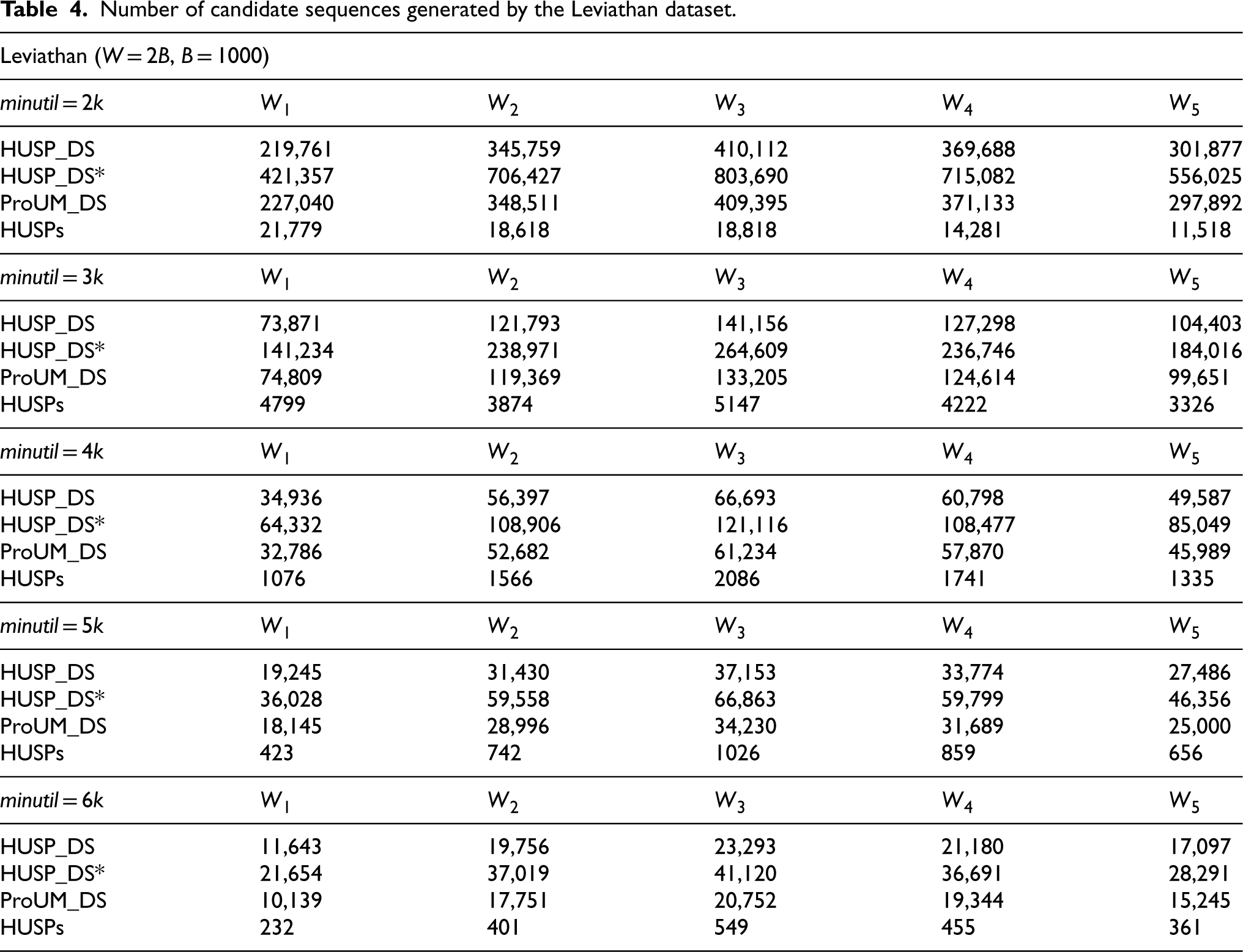
The number of candidate sequences generated by the algorithm on the Leviathan dataset is shown in Table 4, where the window size is set to 2B, batch size to 1000, and minutil ranges from 2000 to 6000 to observe the experimental results under different thresholds. It is worth noting that the sets of pattern results mined by the three algorithms are consistent. From Table 4, it can be seen that the HUSP_DS* algorithm generates the most candidate sequences, approximately doubling compared to HUSP_DS and ProUM_DS. When the minimum utility threshold is 2000, the HUSP_DS algorithm generates 219761 candidate sequences in the first window, while ProUM_DS shows a 3% increase in the number of sequences generated. With a threshold of 6000, ProUM_DS generates 10139 candidate sequences in the first window, representing a 15% increase in the number of sequences generated by the HUSP_DS algorithm. However, in most cases, there is little difference in the number of candidate sequences generated by the HUSP_DS and ProUM_DS algorithms. This is because the Leviathan dataset contains a large number of unique items and has a relatively small overall database size, causing high utility sequential patterns to be less affected by each sequence record in the database. Therefore, the pruning strategies used by both the ProUM_DS and HUSP_DS algorithms do not show significant differences.

Table 4.

Number of candidate sequences generated by the Leviathan dataset.

Leviathan (W = 2B, B = 1000)
minutil = 2k	W ₁	W ₂	W ₃	W ₄	W ₅
HUSP_DS	219,761	345,759	410,112	369,688	301,877
HUSP_DS*	421,357	706,427	803,690	715,082	556,025
ProUM_DS	227,040	348,511	409,395	371,133	297,892
HUSPs	21,779	18,618	18,818	14,281	11,518
minutil = 3k	W ₁	W ₂	W ₃	W ₄	W ₅
HUSP_DS	73,871	121,793	141,156	127,298	104,403
HUSP_DS*	141,234	238,971	264,609	236,746	184,016
ProUM_DS	74,809	119,369	133,205	124,614	99,651
HUSPs	4799	3874	5147	4222	3326
minutil = 4k	W ₁	W ₂	W ₃	W ₄	W ₅
HUSP_DS	34,936	56,397	66,693	60,798	49,587
HUSP_DS*	64,332	108,906	121,116	108,477	85,049
ProUM_DS	32,786	52,682	61,234	57,870	45,989
HUSPs	1076	1566	2086	1741	1335
minutil = 5k	W ₁	W ₂	W ₃	W ₄	W ₅
HUSP_DS	19,245	31,430	37,153	33,774	27,486
HUSP_DS*	36,028	59,558	66,863	59,799	46,356
ProUM_DS	18,145	28,996	34,230	31,689	25,000
HUSPs	423	742	1026	859	656
minutil = 6k	W ₁	W ₂	W ₃	W ₄	W ₅
HUSP_DS	11,643	19,756	23,293	21,180	17,097
HUSP_DS*	21,654	37,019	41,120	36,691	28,291
ProUM_DS	10,139	17,751	20,752	19,344	15,245
HUSPs	232	401	549	455	361

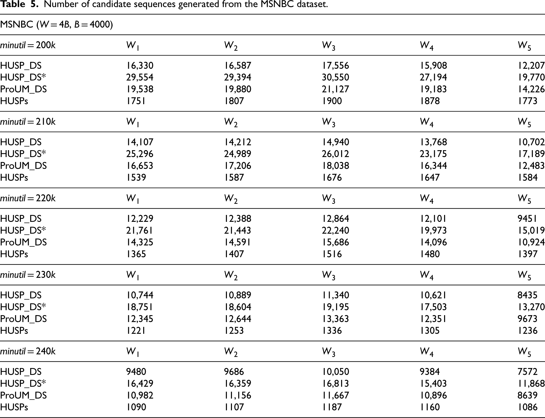
The number of candidate sequences generated by the three algorithms on the MSNBC dataset is shown in Table 5, the pattern result sets they mine is consistent, where the window size is set to 4B, batch size to 4000, and minutil ranges from 200k to 240k to observe the experimental results under different thresholds. On the MSNBC dataset, the HUSP_DS algorithm generates the fewest candidate sequences. When the threshold is 200k, the number of candidate patterns generated by HUSP_DS is approximately 20% fewer than ProUM_DS and 80% fewer than HUSP_DS*. When the threshold is 240k, HUSP_DS still generates the fewest candidate sequences, with approximately 15% fewer than ProUM_DS and 35% fewer than HUSP_DS* algorithm. From these results, it can be concluded that compared to similar algorithms, the proposed algorithm in this paper generates relatively fewer candidate sequences during the mining process.

Table 5.

Number of candidate sequences generated from the MSNBC dataset.

MSNBC (W = 4B, B = 4000)
minutil = 200k	W ₁	W ₂	W ₃	W ₄	W ₅
HUSP_DS	16,330	16,587	17,556	15,908	12,207
HUSP_DS*	29,554	29,394	30,550	27,194	19,770
ProUM_DS	19,538	19,880	21,127	19,183	14,226
HUSPs	1751	1807	1900	1878	1773
minutil = 210k	W ₁	W ₂	W ₃	W ₄	W ₅
HUSP_DS	14,107	14,212	14,940	13,768	10,702
HUSP_DS*	25,296	24,989	26,012	23,175	17,189
ProUM_DS	16,653	17,206	18,038	16,344	12,483
HUSPs	1539	1587	1676	1647	1584
minutil = 220k	W ₁	W ₂	W ₃	W ₄	W ₅
HUSP_DS	12,229	12,388	12,864	12,101	9451
HUSP_DS*	21,761	21,443	22,240	19,973	15,019
ProUM_DS	14,325	14,591	15,686	14,096	10,924
HUSPs	1365	1407	1516	1480	1397
minutil = 230k	W ₁	W ₂	W ₃	W ₄	W ₅
HUSP_DS	10,744	10,889	11,340	10,621	8435
HUSP_DS*	18,751	18,604	19,195	17,503	13,270
ProUM_DS	12,345	12,644	13,363	12,351	9673
HUSPs	1221	1253	1336	1305	1236
minutil = 240k	W ₁	W ₂	W ₃	W ₄	W ₅
HUSP_DS	9480	9686	10,050	9384	7572
HUSP_DS*	16,429	16,359	16,813	15,403	11,868
ProUM_DS	10,982	11,156	11,667	10,896	8639
HUSPs	1090	1107	1187	1160	1086

From the above experiments, it can be observed that the choice of different threshold values significantly affects the algorithm's time and space efficiency. The HUSP_DS algorithm consistently outperforms other algorithms in terms of efficiency across various threshold settings. Therefore, the HUSP_DS algorithm is well-suited for mining high utility sequential patterns in data streams.

5.3 Experimental results with different windows and batch sizes

The window size and batch size are two crucial parameters in the sliding window model. The experiment involves fixing the minimum utility threshold (minutil) and varying the window size (WinSize) and batch size (BatchSize) to compare the algorithm's runtime and memory consumption.

Firstly, the impact of different window sizes on algorithm performance is analyzed. The window size represents the number of batches contained in the window, while the batch size indicates the number of sequences in each batch. The experiment maintains a fixed minimum utility threshold and batch size, examining the algorithm's spatiotemporal efficiency under different window sizes. For the BIKE dataset, with minutil = 2800 and BatchSize = 5000, WinSize ∈[1,5]. Similarly, for the Leviathan dataset, minutil = 3000, BatchSize = 1000, and WinSize ∈ [1,5]. For the MSNBC dataset, minutil =100000, BatchSize = 5000, and WinSize ∈ [1,5]. As shown in Figure 10, HUSP_DS proves to be the fastest algorithm across all datasets. Particularly noteworthy is the comparison on the BIKE dataset, where ProUM_DS consumes 2–4 times more runtime than HUSP_DS and 2–3 times more than HUSP_DS when the window size is 5B. The significant reduction in runtime for all algorithms when the window size is 5B is attributed to the window encompassing all sequences in the dataset. The algorithms adopt a single-window approach for mining, eliminating the need for batch insertions and deletions, thereby reducing runtime. On the Leviathan dataset, the runtime increases proportionally with the window size. HUSP_DS consistently exhibits the minimum average runtime, demonstrating approximately 11% and 79% lower consumption compared to HUSP_DS* and ProUM_DS, respectively. For the MSNBC dataset, when the window size increases from 2B to 3B, ProUM_DS experiences a runtime increase of 398.3%, while HUSP_DS* and HUSP_DS increase by 276.5% and 229.8%, respectively. Additionally, when the window size exceeds 5B, ProUM_DS fails to mine patterns within a limited time.

Figure 10.

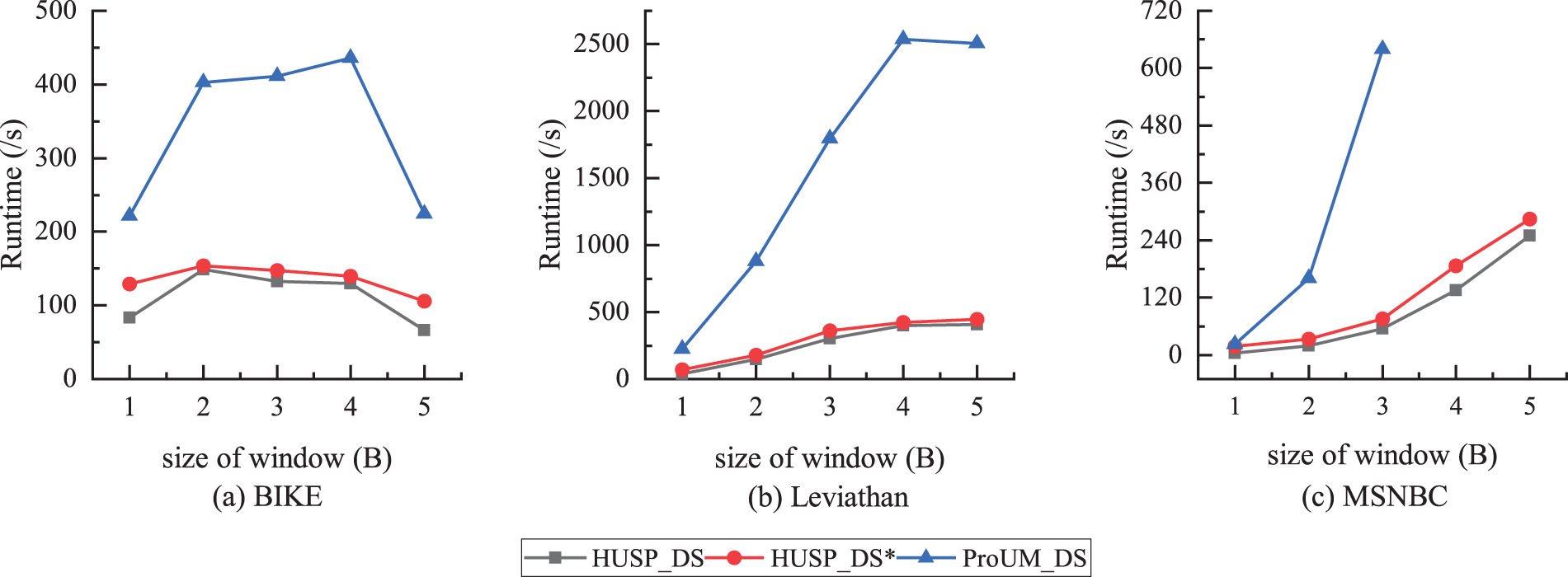
Comparison of running time under different window sizes.

Figure 11 illustrates the maximum memory consumption for the three algorithms under different window sizes. HUSP_DS consistently exhibits the lowest memory consumption, with an average of approximately 4554.18MB on the BIKE dataset. In contrast, HUSP_DS* and ProUM_DS experience an average memory consumption increase of 10% and 16%, respectively. The observed increase in memory usage with larger window sizes is attributed to a decrease in the number of generated windows, leading to a reduction in the frequency of mining operations. However, the increased number of sequences within each window necessitates the construction of additional data structures, consequently increasing memory usage. Overall, these results strongly support the suitability of the proposed algorithm for mining high utility sequential patterns within sliding windows of any size.

Figure 11.

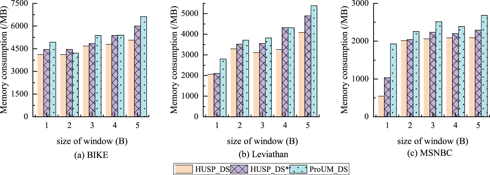
Comparison of memory consumption under different window sizes.

The number of efficient sequence patterns mined by the three algorithms is shown in Figure 12. It can be seen that the number of patterns mined on BIKE, Leviathan, and MSNBC is consistent.

Figure 12.

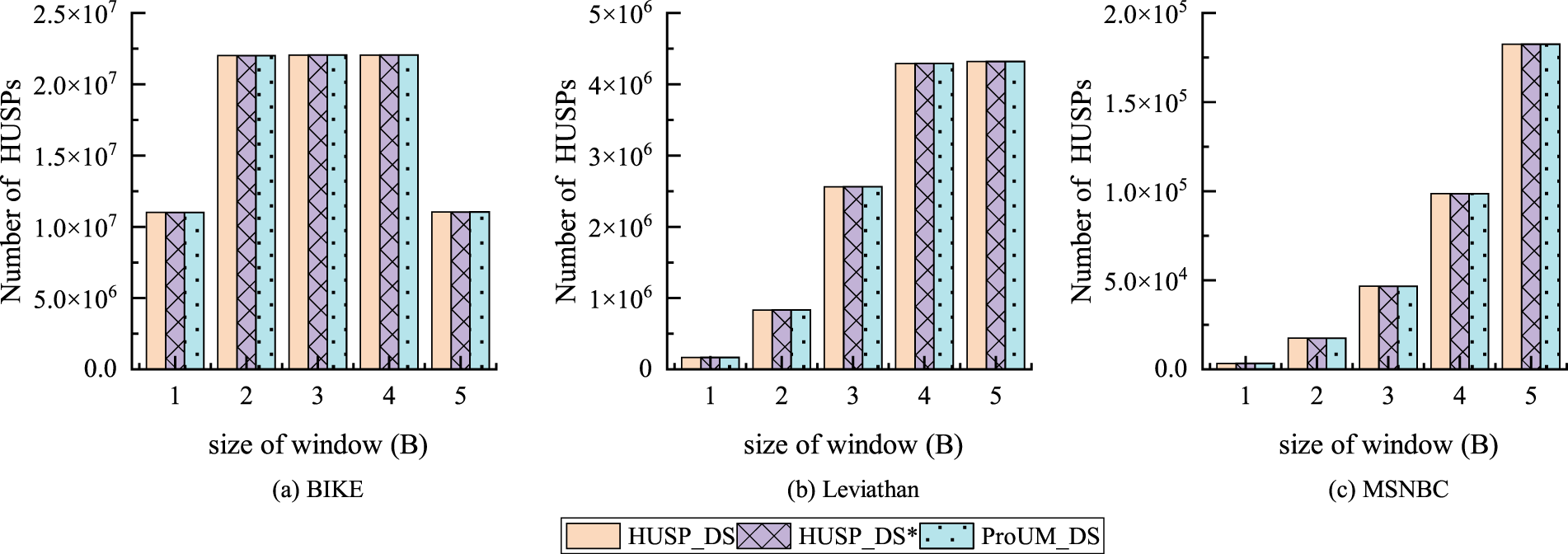
Number of patterns under different window sizes.

Next, the impact of different batch sizes on algorithm performance is analyzed. Considering the BIKE dataset, with minutil = 2800, WinSize = 2, and BatchSize $\in$ [1000,5000]. For the Leviathan dataset, minutil = 3000, WinSize = 3, and BatchSize $\in$ [1000,1800]. For the MSNBC dataset, minutil = 500,000, WinSize = 5, and BatchSize $\in$ [1000,5000]. The experimental results are depicted in Figure 13, where the overall trend shows an increase in runtime with an increase in batch size for all algorithms. On the BIKE and Leviathan datasets, there is a decrease in runtime with an increase in batch size. This is attributed to the increased number of sequences in each batch, which, to some extent, reduces the frequency of sliding window creations and algorithm mining executions, resulting in reduced runtime. Overall, HUSP_DS exhibits average time consumption of 133 s, 59 s, and 7 s on BIKE, Leviathan, and MSNBC datasets, respectively. The runtime increases for HUSP_DS is approximately 112%, 111%, and 200% on the respective datasets. In comparison, ProUM_DS experiences an average runtime increase of approximately 315%, 595%, and 500%.

Figure 13.

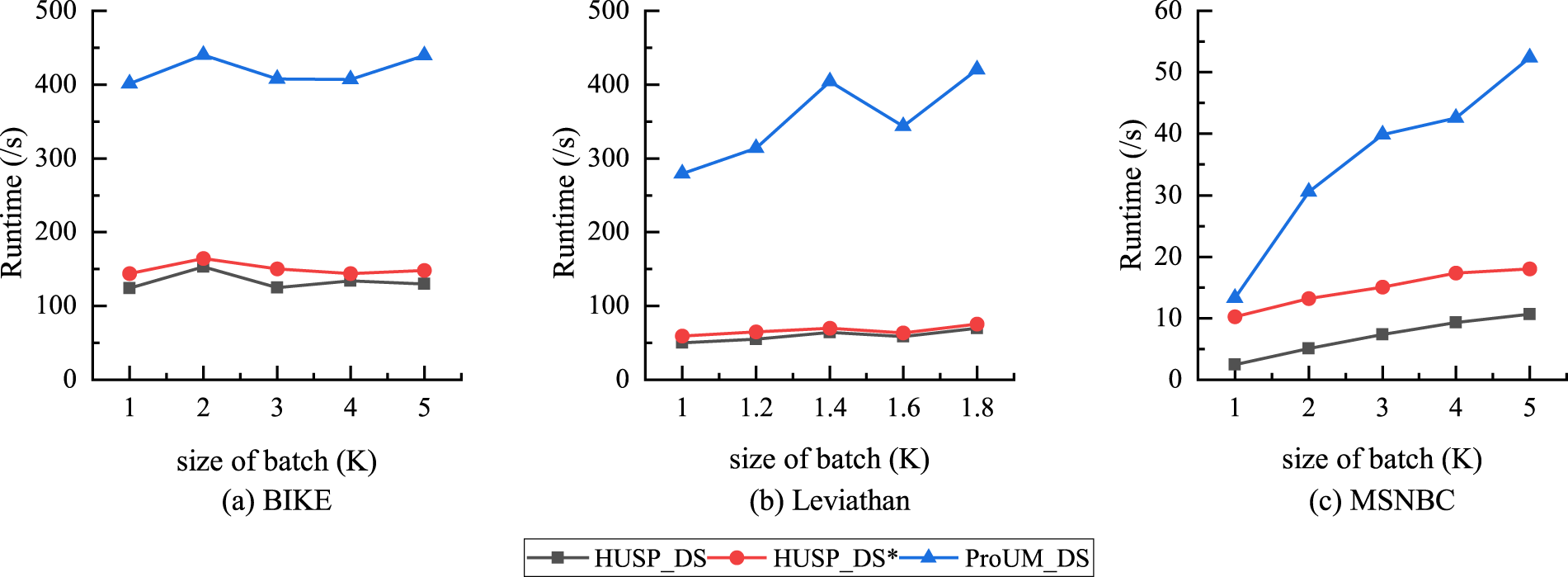
Comparison of runtime with different batch sizes.

The experimental results for memory consumption of the three algorithms are illustrated in Figure 14. On BIKE and Leviathan datasets, the memory consumption for all algorithms shows a relatively small increase, tending towards a stable state. On the MSNBC dataset, HUSP_DS exhibits 65% less memory consumption than ProUM_DS. Therefore, the proposed algorithm in this paper demonstrates the ability to mine high utility sequential patterns under varying batch sizes.

Figure 14.

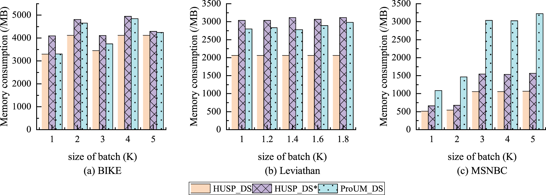
Comparison of memory consumption with different batch sizes.

The number of high utility sequential patterns mined by the three algorithms is shown in Figure 15. It can be observed that, on the BIKE, Leviathan, and MSNBC datasets, the number of patterns mined is consistent across different batch sizes.

Figure 15.

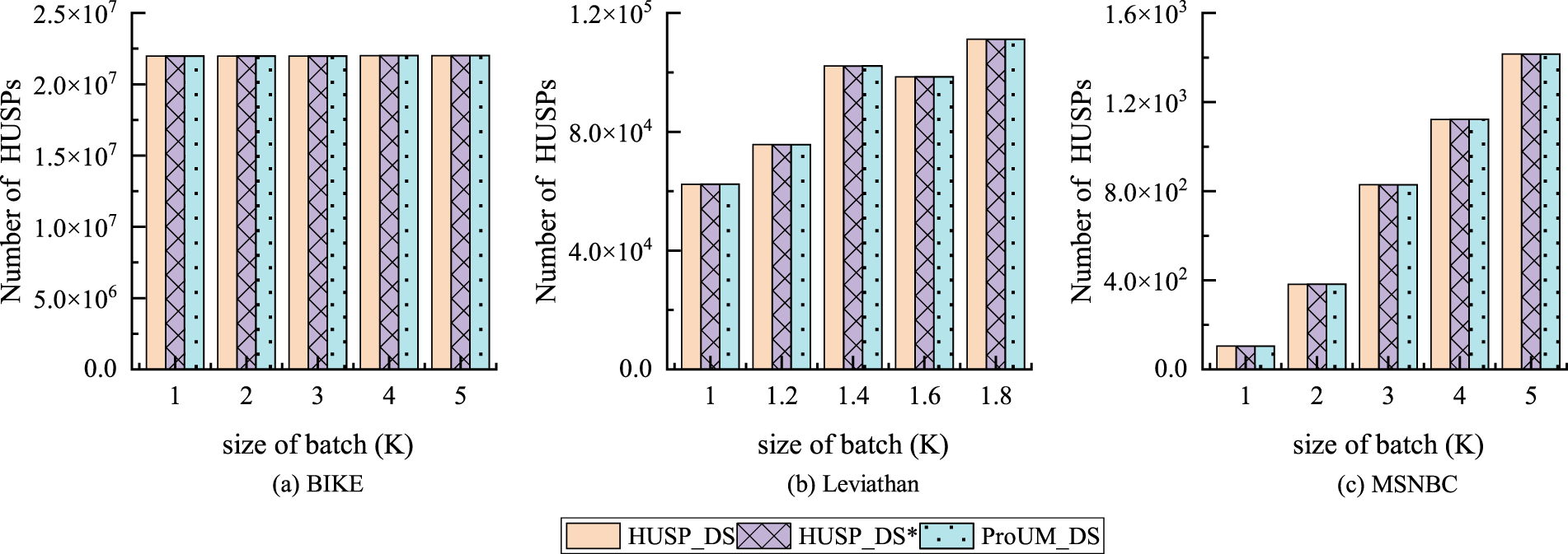
Number of patterns with different batch sizes.

In conclusion, the comprehensive analysis of the experiments reveals that the HUSP_DS algorithm performs well in terms of runtime and memory consumption under different window and batch sizes. It is suitable for mining high utility sequential patterns within windows of arbitrary sizes.

5.4 Scalability test

This section conducts scalability tests on the synthetic dataset S10I5E2D|x|K, as presented in Table 2. The experimental results are illustrated in Figure 16 and Table 6. The experiments were conducted with a minimum utility threshold of 20,000, window size of 3B, and batch size of 20,000 on dataset S10I5E2D|x|K, varying the value of x from 100 to 500.

Figure 16.

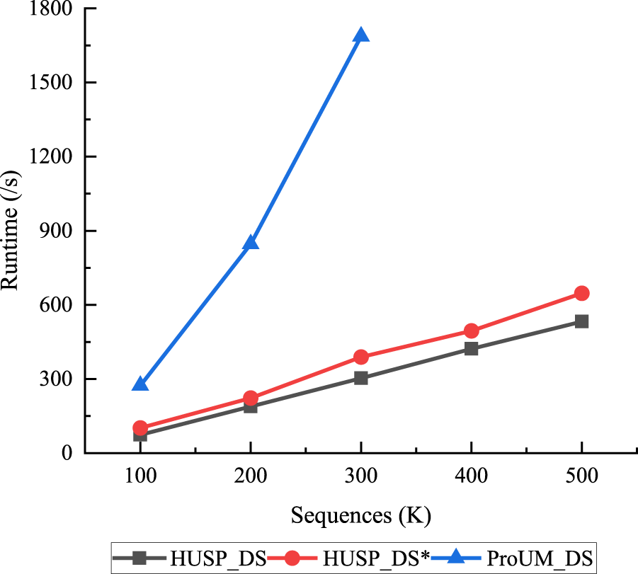
Time scalability test.

Table 6.

Memory scalability test (MB).

DataStream	HUSP_DS	HUSP_DS*	ProUM_DS
100,000	482.08	599.51	639.46
200,000	582.16	763.11	2161.45
300,000	592.11	939.39	2200.13
400,000	642.71	1391.13	–
500,000	690.78	1460.05	–

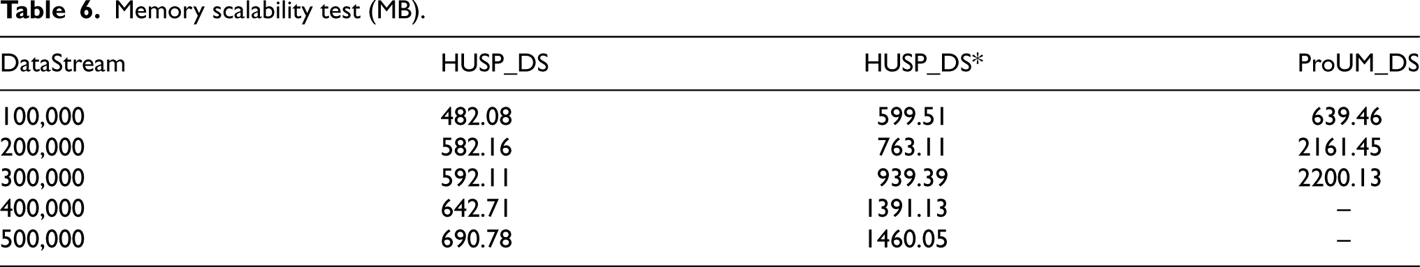
The analysis of the experimental results indicates a linear increase in both time and space efficiency as the data stream size grows. The HUSP_DS algorithm, leveraging a sliding window model and focusing solely on the current window's sequences, efficiently updates transactions in real-time, swiftly discovering high utility sequential patterns. This advantageous approach results in superior runtime and memory consumption. The outcomes demonstrate that the HUSP_DS algorithm exhibits excellent performance on large datasets, showcasing strong scalability and suitability for handling big data.

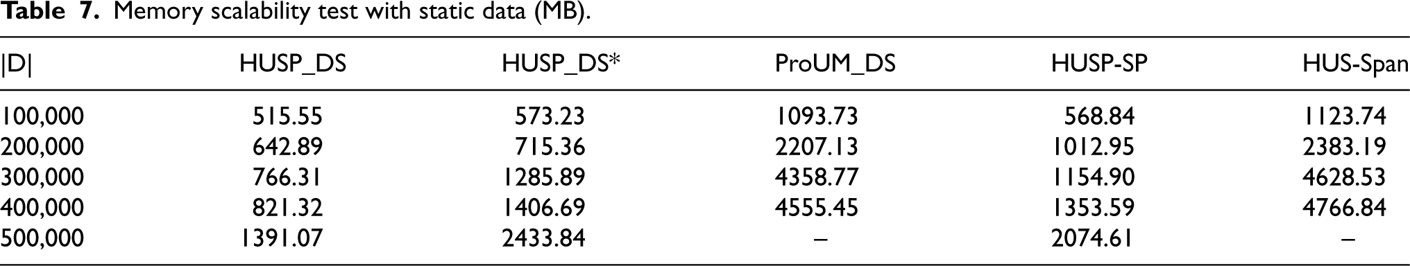
To test the performance comparison between the proposed algorithm and state-of-the-art static algorithms, this study compares the proposed algorithm with HUSP-SP²⁴ and HUS-Span,¹⁹ with a threshold set at minutil = 0.03%. The proposed algorithm and the ProUM_DS algorithm are both operated in a single-window manner (with window size set to 1 and batch size set to the dataset size). The experimental results are shown in Figure 17 and Table 7. Among all the test results, the HUSP_DS algorithm shows the lowest runtime and memory consumption, demonstrating the best scalability among all compared algorithms. From Figure 17, it is observed that the runtime of the HUSP_DS algorithm linearly increases with the number of sequences in the data stream. The table indicates that the memory consumption of the HUSP_DS algorithm remains relatively stable. These results indicate that compared to existing static algorithms, the scalability of the HUSP_DS algorithm is optimal for large-scale datasets, making it suitable for handling big data.

Figure 17.

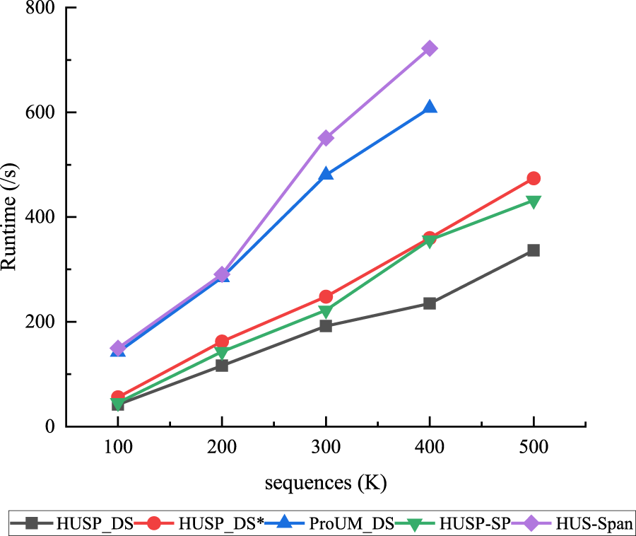
Time scalability test with static data.

Table 7.

Memory scalability test with static data (MB).

\|D\|	HUSP_DS	HUSP_DS*	ProUM_DS	HUSP-SP	HUS-Span
100,000	515.55	573.23	1093.73	568.84	1123.74
200,000	642.89	715.36	2207.13	1012.95	2383.19
300,000	766.31	1285.89	4358.77	1154.90	4628.53
400,000	821.32	1406.69	4555.45	1353.59	4766.84
500,000	1391.07	2433.84	–	2074.61	–

6 Conclusion

To tackle the challenge of efficiently extracting high utility sequential patterns from dynamically changing data streams, this study introduces a novel algorithm. Firstly, addressing the inefficiencies in existing algorithms for mining high utility sequential patterns in data streams, this paper presents a new structure called DUI-table, serving as a dynamic utility index table. This structure optimally reduces the search space using a prefix recursive projection mechanism, allowing for swift and accurate construction and updating of abundant information in the sequential data of the data stream. The DUI-table proves to be well-suited for mining high utility sequential patterns in data streams. Secondly, based on the DUI-table structure, a data stream high utility sequential pattern mining algorithm is devised. This algorithm employs a sliding window model for real-time discovery of valuable patterns. Finally, to evaluate the effectiveness of the proposed algorithm, extensive experiments are conducted on both real and synthetic datasets. The results demonstrate that the HUSP_DS algorithm can efficiently mine high utility sequential patterns in data streams with arbitrary window and batch sizes, showcasing strong scalability. In summary, HUSP_DS provides a feasible and effective solution for mining high utility sequential patterns in complex and dynamic data stream environments.

In addition, this algorithm faces two key issues: the difficulty in setting the minimum utility threshold and handling the oldest batch within a window and the common batch between two adjacent windows. First, in the process of mining high utility sequential patterns in data streams, multiple experiments are required to validate the threshold's effectiveness, or the threshold is set based on expert experience. However, users lack sufficient prior knowledge, resulting in difficulty in setting the threshold. Second, the sliding window used by this algorithm focuses on the value generated by recent data, neglecting the value generated by historical data. Additionally, the common batches between two sliding windows need to be re-mined, which increases spatiotemporal consumption. Therefore, considering the value generated by historical data and reducing the number of re-mining of common batches based on the result set of the previous window are issues that need further resolution by this algorithm. For the first issue, an effective solution is to not set a minimum utility threshold but directly mine the top k patterns with the highest utility values. Therefore, future research can focus on introducing a self-adaptive selection mechanism for the minimum utility threshold to improve the algorithm's robustness and application scope. For the second issue, overlapping windows can capture more events, reducing the possibility of missed events. They can also flexibly adjust the sliding step to meet various data processing needs. However, this also brings the drawback of repeated mining in overlapping windows and neglecting the value generated by historical data. Therefore, future work can focus on combining the advantages of both landmark windows and sliding windows to mine high utility sequential patterns in data streams.

Footnotes

Acknowledgements

This research was supported by the National Natural Science Foundation of China (62062004), the Natural Science Foundation of Ningxia (2023AAC03315), the Central Universities Foundation of North Minzu University (2021KJCX10), and the Graduate Innovation Project of North Minzu University (YCX24120).

ORCID iD

Meng Han

Credit authorship contribution statement

Meng Han: Supervision, Writing, Reviewing. Ruihua Zhang: Conceptualization, Methodology, Writing-original draft. Feifei He: Data curation, Writing-original draft. Fanxing Meng and Chunpeng Li: Co-supervision, Writing, Editing.

Funding

The author(s) disclosed receipt of the following financial support for the research, authorship, and/or publication of this article: This research was supported by the National Natural Science Foundation of China (62062004), the Natural Science Foundation of Ningxia (2023AAC03315), the Central Universities Foundation of North Minzu University (2021KJCX10), and the Graduate Innovation Project of North Minzu University (YCX24120).

Declaration of conflicting interests

The authors declared no potential conflicts of interest with respect to the research, authorship, and/or publication of this article.

References

Yin

Zheng

Cao

. USpan: an efficient algorithm for mining high utility sequential patterns. In: Proceedings of the 18th ACM SIGKDD international conference on knowledge discovery and data mining (KDD), 2012, pp.660–668.

Dong

Gong

Cao

. e-RNSP: an efficient method for mining repetition negative sequential patterns. IEEE Trans Cybern (TCYB) 2018; 50: 2084–2096.

Gan

Huang

, et al. Targeted mining of contiguous sequential patterns. Inf Sci (INS) 2024; 653: 119791.

Han

. Research on closed pattern-based data mining technologies. Beijing jiaotong University (BJTU), 2016, pp.17–18.

Zihayat

Chen

. Memory-adaptive high utility sequential pattern mining over data streams. Mach Learn (ML) 2017; 106: 799–836.

Kim

Yun

. Mining high utility itemsets based on the time decaying model. Intell Data Anal (IDA) 2016; 20: 1157–1180.

Yun

Kim

Yoon

, et al. Damped window based high average utility pattern mining over data streams. Knowl-Based Syst (KBS) 2018; 144: 188–205.

Zihayat

, et al., Efficiently mining high utility sequential patterns in static and streaming data. Intell Data Anal (IDA) 2017; 21(S1): S103–S135.

Cheng

Han

Zhang

, et al. Closed high utility itemsets mining over data stream based on sliding window model. J Comput Res Dev (JCRD) 2021; 58: 2500–2514.

10.

Han

Chen

, et al. FCHM-stream: fast closed high utility itemsets mining over data streams. Knowl Inf Syst (KAIS) 2023; 65: 2509–2539.

11.

Han

Liu

Gao

, et al. Mining top-K constrained cross-level high-utility itemsets over data streams. Knowl Inf Syst (KAIS) 2024; 66: 2885–2924.

12.

Tang

Liu

Wang

. A new algorithm of mining high utility sequential pattern in streaming data. Int J Comput Intell Syst (IJCIS) 2018; 12: 342–350.

13.

Ishita

Ahmed

Leung

. New approaches for mining regular high utility sequential patterns. Appl Intell (APIN) 2022; 52: 3781–3806.

14.

Ahmed

Tanbeer

Jeong

. Mining high utility web access sequences in dynamic web log data. In: Proceedings of 2010 11th ACIS international conference on software engineering, artificial intelligence, networking and parallel/distributed computing, IEEE, 2010, pp.76–81.

15.

Ahmed

Tanbeer

Jeong

. A novel approach for mining high-utility sequential patterns in sequence databases. ETRI J 2010; 32: 676–686.

16.

Shie

Hsiao

Tseng

, et al. Mining high utility mobile sequential patterns in mobile commerce environments. In: Proceedings of the 16th international conference on database systems for advanced applications (DASFAA), Hong Kong, China, April 22–25 2011. Berlin, Heidelberg: Springer, 2011, pp.224–238.

17.

Yin

Zheng

Cao

, et al. Efficiently mining top-k high utility sequential patterns. In: Proceedings of the 2013 IEEE 13th international conference on data mining (ICDM). IEEE, 2013, pp.1259–1264.

18.

Alkan

Karagoz

. CRom and HuspExt: improving efficiency of high utility sequential pattern extraction. IEEE Trans Knowl Data Eng (TKDE) 2015; 27: 2645–2657.

19.

Wang

Huang

Chen

. On efficiently mining high utility sequential patterns. Knowl Inf Syst (KAIS) 2016; 49: 597–627.

20.

Gan

Lin

JCW

Zhang

, et al. ProUM: projection-based utility mining on sequence data. Inf Sci (INS) 2020; 513: 222–240.

21.

Gan

Lin

JCW

Zhang

, et al. Fast utility mining on sequence data. IEEE Trans Cybern (TCYB) 2020; 51: 487–500.

22.

Zhang

Gan

, et al. TKUS: mining top-k high utility sequential patterns. Inf Sci (INS) 2021; 570: 342–359.

23.

Zhang

Yang

, et al. On-shelf utility mining of sequence data. ACM Trans Knowl Discov Data (TKDD) 2021; 16: 1–31.

24.

Zhang

Yang

, et al. HUSP-SP: faster utility mining on sequence data. ACM Trans Knowl Discov Data (TKDD) 2023; 18: 1–21.

25.

Zhang

Han

, et al. A survey of high utility sequential patterns mining methods. J Intell Fuzzy Syst (JIFS) 2023; 45: 8049–8077.

26.

Ayres

Flannick

Gehrke

, et al. Sequential pattern mining using a bitmap representation. In: Proceedings of the eighth ACM SIGKDD international conference on knowledge discovery and data mining (KDD), 2002, pp.429–435.

An efficient algorithm for high utility sequential pattern mining over data streams based on sliding window model

Abstract

Keywords

1 Introduction

2.1 High utility sequential pattern mining

2.2 High utility sequential pattern mining over data streams

3 Preliminaries

4.1 Search space and pruning strategy

4.1.1 Search space

5 Experiments

5.1 Experimental environment and datasets

Table 2. Basic characteristics of the experimental dataset. Datasets |D| Items Lavg Element BIKE 21,078 67 7.28 1.00 Leviathan 5834 9025 33.81 1.00 MSNBC 31,790 17 13.33 1.00 S10I5E2D|x|K x*1000 9999 8.98 2.00

Footnotes

Acknowledgements

ORCID iD

Credit authorship contribution statement

Funding

Declaration of conflicting interests

References

Table 2.
Basic characteristics of the experimental dataset.

Datasets |D| Items L_avg Element

BIKE 21,078 67 7.28 1.00

Leviathan 5834 9025 33.81 1.00

MSNBC 31,790 17 13.33 1.00

S10I5E2D|x|K x*1000 9999 8.98 2.00