The Contribution of US Taxes and Social Transfers to Income Redistribution

Abstract

The aim of this work is to solve the problem of nonadditivity revealed by work that calculates the redistributive effects of the budget or public policies made up of different instruments of income or public spending. To do this, the authors use the Shapley value. This technique allows us to consistently, symmetrically, and directly decompose the redistributive effect and the vertical and horizontal effects. This method is consistent because the total effects can be explained by the sum of the individual contributions; it is symmetrical because it does not depend on the aggregation ranking of the instruments; and it is direct because each index can be calculated without the need to calculate the rest. The main result obtained for the case of taxes and social transfers in the United States is that previous calculations undervalued the redistributive effects and their vertical and horizontal components for taxes and transfers. Undervaluation is more important for taxes.

Keywords

redistributive effects decomposition taxes welfare expenditures JEL: H23,D31,138

Within public economy studies, there is an important tradition in the analysis of the redistributive effects of taxes. One of the most widely used indicators to calculate redistributive effects is the difference in Gini indexes before and after taxes (Reynolds and Smolensky 1977). Its versatility and simplicity has meant the extending of the measure to all kinds of public intervention instruments and even to the analysis of the redistributive effect of the whole budget.¹ An additional development is in decomposing the Reynolds–Smolensky index to assess the effects on vertical equity (V^K ) and reranking (R), according to the method of Kakwani (1984), or also on horizontal inequality (H), according to the proposal of Aronson, Johnson, and Lambert (1994).²

The problem of works that calculate the redistributive impacts of policies made up of various instruments or the whole budget is that they tend to present inconsistent results. Additive inconsistence is produced when the sum of the redistributive effects of each instrument does not coincide with the redistributive effect of the measures taken as a whole. This nonadditivity is due to calculating the redistributive effects of each instrument, excluding the other instruments; that is, the interaction between instruments having an effect on the redistributive effect is not taken into account (Lambert 1985, 46).

An elemental solution is to sequentially aggregate the different instruments to calculate their redistributive impacts.³ The problem that this solution produces is that the redistributive effects calculated for the same instrument are different according to the sequence chosen (Lambert 1985, 43; asymmetrical results); that is, we are faced with a problem of judgment values due to the author opting for a specific sequence.

Another means of analysis is to determine the contribution of each instrument via a procedure of decomposing the effect of the net budget. The first one proposed was by Lambert (1985), who decomposed the vertical effect of the net budget in the sum of the vertical effects of taxes and transfers. This V decomposition is equivalent to decomposing RE when there is no reranking. However, in the case of reranking, Lambert’s method does not allow RE to be estimated for each instrument. Although this decomposition is the most widely accepted and used, it only offers analytical information about vertical equity.

Other authors have tried to advance in the decomposition of R, for instance, Jenkins (1988), Duclos (1993), and more recently Urban (2010). Jenkins (1988) shows that Lambert’s estimates of RE will be biased because reranking has not been taken into account, so he decomposes the redistributive effect of the net budget. The redistributive effect of each instrument is expressed in terms of Reynolds-Smolensky index and not of Kakwani’s V, as Lambert (1985) does, and the sum of the contributions of the taxes and the benefits of the reranking does not coincide with the total reranking, as a residue appears that makes the solution inconsistent.

Duclos (1993) maintains the decomposition of V according to Lambert (1985), and to decompose R uses the sequential method, so that for m instruments m! possible sequences are obtained. For four instruments, he obtains twelve possible values of reranking without opting for any of them and therefore without giving a specific result of the disaggregation of R. As we see later on, the methodology that we propose maintains a certain connection with the work of Duclos in that it averages out the value of all the possible values resulting from all the sequences.

More recently, Urban (2010) has proposed a complex method of additively decomposing RE, V, and R. His article analyzes differences in incomes, taxes, and benefits for pairs of income units. Afterward, these differences are aggregated across the population and averaged. Nevertheless, since these calculations assume budgetary balance, when this does not hold true he has to introduce counterfactual tax and benefit variables. He uses two ways of building the counterfactual variables, with different criteria. With this methodology Urban obtains two different decompositions, and one of them offers V values equal to those found by Lambert, although R cannot straightforwardly be directly decomposed in the same manner as V. To solve this, Urban uses a criterion of spreading the reranking for the pair of units (i, j), as by a weight that represents the share of tax or benefit in total T&Bs—at the level of the pair (i, j). Understandably, such a weight is different according to the counterfactual vector chosen. Finally, he calculates the RE of each instrument as the difference between V and R for each pair.

To sum up, the methodologies used until now to decompose RE, V, H, and R are either incomplete, such as Lambert’s (1985), produce a residue, as with Jenkins's (1988), or force the establishing of assumptions that condition the result, as in the sequential solution of Duclos (1993) or Urban (2010). To solve these problems, we propose adapting the Shapley value, a method that spreads the joint effects that come from game theory, to the decomposition of the redistributive effects.

This methodology consists of calculating, for each financial instrument, the average marginal effect of all the possible sequences in which the instrument could appear. Shorrocks (1999) encouraged the use of the Shapley value in order to decompose inequality indicators. This methodology has been widely used in breaking down poverty indicators (Kolenikov and Shorrocks 2005; Deustch and Silber 2008; Bibi and Duclos 2010). But, unlike Shorrocks, in our work we apply it to the variation of inequality indexes (RE, V, H, and R).

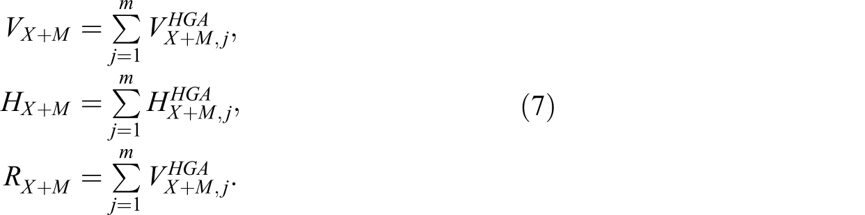
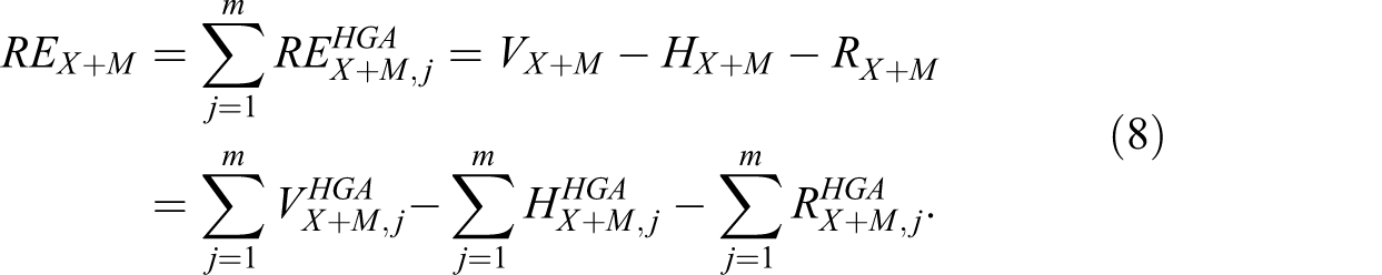
We thus manage to calculate the individual contribution of taxes and benefits to the redistributive effects of the net budget, in the following denominated V^HGA, H^HGA, R^HGA , and RE^HGA. The result is consistent (the individual effects of the various financial instruments explain the total effect of the whole fiscal system), symmetrical (the order in which the instruments are added does not affect the results) and direct; that is to say, we do not need to calculate the decomposition of any index to determine the other. Thus, R or RE can be decomposed without the need to calculate V.

We also compare the result that we obtain for the decomposition of V, V^HGA , with that obtained by Lambert (1985), V^L , which is the most widely used. Both indexes are obtained as a weighted average of Kakwani’s progressivity index, although they differ in their weights, and in V^HGA a second element appears that is not in V^L . This second element evaluates the incidence of an instrument in the vertical equity of the other. These differences allow us to provide an explanation of Lambert’s paradox, according to which the vertical effect of the net budget can be greater than the vertical effect of the benefits in spite of the taxes being regressive, according to Kakwani’s progressivity index.

Finally, our reference for presenting analytical results is a recent work by Kim and Lambert (2009) in which the redistributive impact is analyzed for taxes and social spending in the United States for the years 1994, 1999, and 2004. Our calculations allow the consistent and symmetrical decomposing of the total redistributive effect, the vertical effect, the horizontal inequality, and the reranking that taxes and social benefits produce in the United States. The result we obtain is that the redistributive effects of taxes and benefits are greater than those calculated, as separate instruments, on the initial income. At the same time, the calculations allow us to conclude that the undervaluing of the redistributive effect is greater in case of the taxes. According to our estimation, the relative weight of the taxes would represent around 25 percent of the total redistribution (RE), which contrasts with 12 percent attributed by Kim and Lambert for 2004, when disaggregating only the vertical effect (V).

This article is organized as follows: in the following section, the methodology that we propose to obtain an additive, symmetrical, and direct decomposition is put forward. In Comparing V^L and V^HGA section, we analyze the connection between the decomposition of V carried out by Lambert (1985) and the methodology here proposed. In Results section, we present the results obtained by applying this methodology to the data provided by Kim and Lambert (2009). The last section summarizes the results obtained and offers some concluding remarks.

Methodology

The most common ways of calculating the vertical and horizontal redistributive effects of taxes are those devised by Kakwani (1984) and by Aronson, Johnson, and Lambert (1994).⁴ The first distinguishes between the vertical effect and reranking:

R E_{X - T} = V_{X - T}^{} - R_{X - T}^{} .

The second also identifies the horizontal inequality without an order change:⁵

R E_{X - T} = V_{X - T}^{} - H_{X - T}^{} - R_{X - T}^{} .

So, the vertical equity (V) effect measures the progressivity, which is positive if the taxation system is progressive and negative if it is regressive. The horizontal inequality (H) relates to an unequal treatment of equals. A further concept of reranking (R) corresponds to the income scale rank-switching induced by the fiscal system.

In theory, for each of the m instruments $j$ , (j = 1,…, m) that make up a policy M we can calculate its respective redistributive effects $R E_{X + j}$ and the problem of inconsistency or asymmetry results from $R E_{X + M} \neq \sum_{j = 1}^{M} R E_{X + j}$ . The same is true for V, H, and R.

A solution can be found to this problem by means of calculating the decomposition via the Shapley (1953) value. This methodology is taken from game theory and has been applied to the study of inequality since the work of Shorrocks (1999). Shapley studies the sharing rule in the case of the joint result not being equal to the sum of the individual results. To that effect, an axiomatic approximation is carried out and requires the sharing criterion to satisfy four requisites:

The sum of the contributions assigned to all the participants explains the joint effect.

If i and j are symmetrical, their contribution is equal.

If j does not change the result, then its contribution is null.

The contribution accumulated by a subset of n elements is the sum of the contribution assigned to each of the n elements.

In his work, Shapley shows that the only rule of sharing that fulfills these axioms is a system that consists of quantifying the impact of a factor by calculating the average of the marginal effects, determined by the elimination of said factor in all the possible sequences. This methodology is called the Shapley value.

Indeed, let M be the set of instruments $j, j \in M = {1, 2, \dots, m}$ , that make up a public policy. Let $G$ be a subset of $M$ made up of $g$ instruments. Let $R E_{X + G}$ be the value of RE when the instruments $j, j \notin G \subseteq M$ have been eliminated. If all the sizes are equally probable, a determined size $g$ will occur with a probability of $1 / g$ . On the other hand, if we have a determined instrument $j$ that belongs to a subgroup $G$ , the $(g - 1)$ instruments remaining of this subgroup can be chosen among the $(m - 1)$ instruments remaining in a number of sequences equal to

\frac{(m - 1)!}{[(m - 1) - (g - 1)]! (g - 1)!} = \frac{(m - 1)!}{(m - g)! (g - 1)!} .

The probability of one of these combinations being chosen is the reciprocal. Therefore, the probability of a group G containing the element

j

is equal to the said reciprocal multiplied by

1 / m

When taken into account the marginal contribution of $j \in G$ to the inequality of the subgroup $G$ , it is as follows:

R E_{X + G, j}^{} = R E_{X + G}^{} - R E_{X + (G - j)}^{} .

The contribution of the instrument $j$ to the total value of the index $R E_{X + M}^{}$ is equal to the summation of all the groupings that can contain it, weighted by the probability of their occurrence:

R E_{X + M, j}^{H G A} = \sum_{\binom{G \subseteq M}{j \in G}} \frac{(m - g)! (g - 1)!}{m!} [R E_{X + G} - R E_{X + (G - j)}]

such that

R E_{X + M} = \sum_{j = 1}^{m} R E_{X + M, j}^{H G A} .

This expression is generalizable to determine the contribution of each

j

to the indices

V_{X + M}^{}

H_{X + M}^{}

and

R_{X + M}^{}

such that

\begin{matrix} V_{X + M} = \sum_{j = 1}^{m} V_{X + M, j}^{H G A}, \\ H_{X + M} = \sum_{j = 1}^{m} H_{X + M, j}^{H G A}, \\ R_{X + M}^{} = \sum_{j = 1}^{m} V_{X + M, j}^{H G A} . \end{matrix}

Therefore,

\begin{aligned} R E_{X + M} = \sum_{j = 1}^{m} R E_{X + M, j}^{H G A} = V_{X + M} - H_{X + M} - R_{X + M}^{} \\ = \sum_{j = 1}^{m} V_{X + M, j}^{H G A} - \sum_{j = 1}^{m} H_{X + M, j}^{H G A} - \sum_{j = 1}^{m} R_{X + M, j}^{H G A} \end{aligned} .

With the Shapley value, the sequence ceases to be determinant. All the possible combinations are considered and the interaction of the instruments that make up the policy is taken into account.

To appreciate the consequences of its application, let’s consider a policy with two instruments, for example taxes (T) and benefits (B), such that for equation (6) it must be met:

R E_{X - T + B} = R E_{X - T + B, T}^{H G A} + R E_{X - T + B, B}^{H G A},

where

\begin{matrix} R E_{X - T + B, T}^{H G A} = \frac{1}{2} (R E_{X - T + B} - R E_{X + B}) + \frac{1}{2} R E_{X - T}, \\ R E_{X - T + B, B}^{H G A} = \frac{1}{2} (R E_{X - T + B} - R E_{X - T}) + \frac{1}{2} R E_{X + B} . \end{matrix}

From these results, Table 1 is assembled, which includes the solution obtained via applying Shapley value and the two possible sequences. Although these latter produce consistent results, they are not symmetrical.

Table 1.

Decomposition of the Redistributive Effect of a Public Policy Made Up of Two Instruments: Taxes and Benefits

Sequence 1 (−t + b)	Sequence 2 (b − t)	Shapley solution
Taxes	$R E_{X - T}$ (I)	$\begin{aligned} R E_{X - T + B} \\ - R E_{X + B} \end{aligned}$ (III)	$\begin{aligned} R E_{T}^{H G A} = \frac{1}{2} (R E_{X - T + B} - R E_{X + B}) \\ + \frac{1}{2} R E_{X - T} (V) \end{aligned}$
Benefits	$\begin{aligned} R E_{X - T + B} \\ - R E_{X - T} \end{aligned}$ (II)	$R E_{X + B}$ (IV)	$\begin{aligned} R E_{B}^{H G A} = \frac{1}{2} (R E_{X - T + B} - R E_{X - T}) \\ + \frac{1}{2} R E_{X + B} (V I) \end{aligned}$
Total	$R E_{X - T + B}$ (VII)	$R E_{X - T + B}$ (VII)	$R E_{X - T + B}$ (VII)

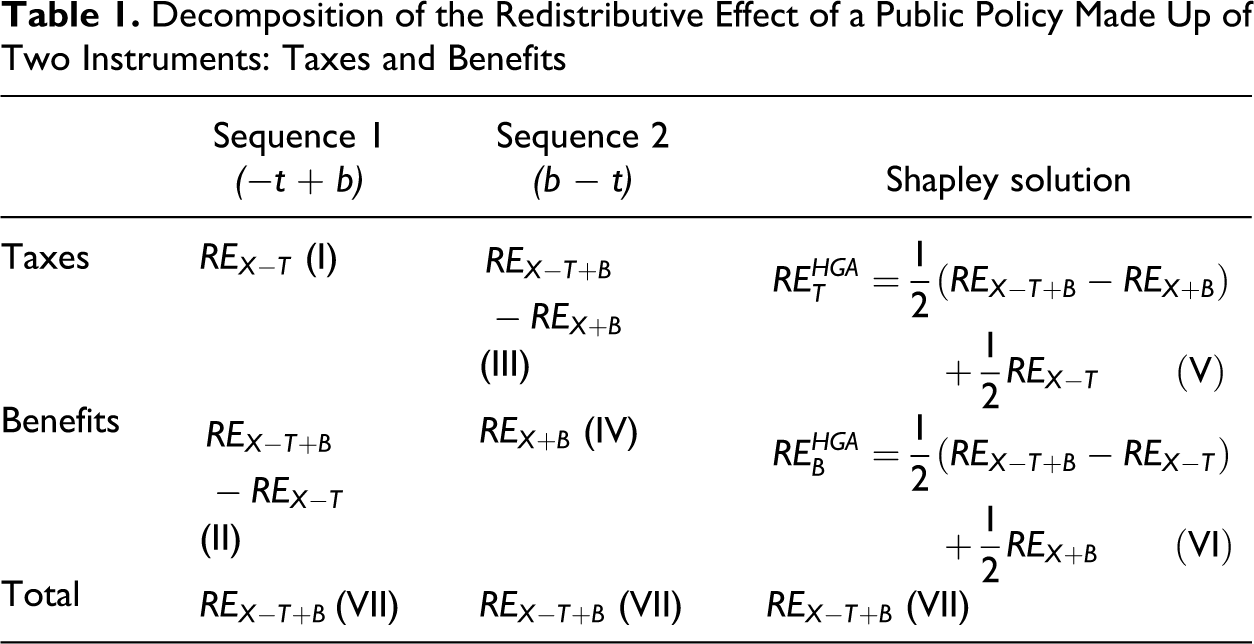
The problem of inconsistency that tends to emerge in works of this kind, as is the case in Kim and Lambert (2009), originates in calculating the total effect, VII, and the effects I and IV. These three effects are estimated as the marginal effect on the initial income; while in VII the interaction of both instruments is taken into account, in I and IV it is not. This inconsistency also results when calculating the partial effects III and II (calculating the redistributive effect of each policy and eliminating it in the final income instead of aggregating it to the initial income), as can be observed in Immervoll et al. (2005).

Shapley’s solution consists of calculating the average of the marginal effects of each instrument in each sequence. It satisfies the properties of additivity and symmetry (V+VI = VII).

Comparing VL and VHGA

As we have pointed out, given the impossibility of additively decomposing R or RE, the usual way in the literature to evaluate the individual contribution of taxes and benefits to the redistributive effect of the net budget is to use the decomposition of V according to Lambert (1985). This can only evaluate the contribution of each instrument to the vertical equity of the net budget.

Lambert (1985) sets out from the evaluation of Kakwani’s vertical equity for each instrument, such that

\begin{aligned} V_{B}^{K} = \frac{b . P_{B}^{K}}{1 + b}, \\ V_{T}^{K} = \frac{t . P_{T}^{K}}{1 - t}, \end{aligned}

where $P_{T}^{K}$ and $P_{B}^{K}$ are the Kakwani progressivity indexes, t the average tax on the initial income, b the average transfer received on the initial income, and (1 − t + b) the final income in proportion to the initial income. Lambert shows that

V_{B}^{K} + V_{T}^{K} \neq V_{B + T}^{K}

and decomposes the vertical effect of the net budget as a weighted average of the progressivity indexes or the Kakwani vertical equity, such that

V_{N}^{L} = \frac{t . P_{T}^{K} + b P_{B}^{K}}{1 - t + b} = \frac{(1 - t) V_{T}^{K} + (1 + b) . V_{B}^{K}}{1 - t + b},

V_{T}^{L} = \frac{t . P_{T}^{K}}{1 - t + b} = \frac{(1 - t) V_{T}^{K}}{1 - t + b},

V_{B}^{L} = \frac{b . P_{B}^{K}}{1 - t + b} = \frac{(1 + b) V_{B}^{K}}{1 - t + b} .

A comparison of V and V^L shows that the decomposition of Lambert increases the absolute value of the vertical equity of the benefits, since, due to the taxes, the transfers have more weight in the final income. On the other hand, the vertical effect of the taxes is always reduced, because, due to the appearance of the benefits, they have less weight in the final income, regardless of both instruments being progressive, regressive or presenting a contrary sign.

Our decomposition proposal, as shown in the annex ( $V_{T}^{H G A}$ $V_{B}^{H G A}$ ), can also be expressed in terms of $V_{}^{L}$ and of $V_{}^{K}$ , so that

V_{T}^{H G A} = 1 / 2 (V_{T}^{L} + V_{T}^{K}) + 1 / 2 (V_{B}^{L} - V_{B}^{K}),

V_{B}^{H G A} = 1 / 2 (V_{B}^{L} + V_{B}^{K}) + 1 / 2 (V_{T}^{L} - V_{T}^{K}) .

In terms of Kakwani’s progressivity indexes, these expressions become

V_{T}^{H G A} = 1 / 2 (\frac{t}{1 - t + b} + \frac{t}{1 - t}) P_{T}^{K} + 1 / 2 (\frac{b}{1 - t + b} - \frac{b}{1 + b}) P_{B}^{K},

V_{B}^{H G A} = 1 / 2 (\frac{b}{1 - t + b} + \frac{b}{1 + b}) P_{B}^{K} + 1 / 2 (\frac{t}{1 - t + b} - \frac{t}{1 - t}) P_{T}^{K} .

The analysis of V^HGA shows how the application of Shapley value considers the interaction between taxes and benefits and the differences with

V_{}^{L}

. To begin with, we analyze the first summation from the right of the equation (14). This contains Kakwani’s progressivity index, the same as V^L , but here it is weighted by the average of the relative weights of the instrument with respect to the income in each possible sequence (1 − t, or 1 + b, and 1 − t + b), and not only with respect to the relative final income (1 − t + b) as in Lambert’s method. Therefore, the first summation considers the impact of the progressivity of the instrument itself on the vertical effect, albeit with different weightings.

Furthermore, each instrument not only has an impact on the vertical effect of the net budget via its own progressivity but also affects the vertical effect of the other instrument, via the change of weighting of the progressivity.

We analyze this second element in the case of taxes, knowing that the initial progressivity of the benefits $P_{B}^{K}$ is weighted by the weight of the benefits b in the final income 1 + b. When we include the taxes, the final relative income is reduced to 1 + b − t and along with it the relative weight of the benefits increases. Moreover, as the two instruments are applied at the same time, the Shapley value confers the taxes with 50 percent of the change in weighting of the progressivity of the benefits, as the probability of the taxes or benefits appearing in the first or second place is half in both cases; that is, the presence of T reinforces the progressivity of B, but unlike Lambert, who considers this as the contribution of B to the vertical equity of the net budget, our method confers a part of this effect on T, as its existence is the cause of B having more weight. Therefore, the difference between $V_{}^{H G A}$ and $V_{}^{L}$ depends on the progressivity or regressivity of T and B, and of the relative weights of the instruments. The relation between $V_{}^{H G A}$ and $V_{}^{L}$ is presented in Table 2 .

Table 2.

Values of VHGA and VL According to the Progressivity of Taxes and Benefits

	Progressive taxes $P_{T}^{K} > 0$	Regressive taxes $P_{T}^{K} < 0$
Progressive Benefits $P_{B}^{K} > 0$	I $V_{T}^{H G A} > V_{T}^{L} > 0$ $V_{B}^{H G A} < V_{B}^{L}$	II $V_{T}^{H G A} < V_{T}^{L} < 0$ $V_{B}^{H G A} > V_{B}^{L} > 0$ if $\frac{1 + b}{1 - t} > - \frac{P_{B}}{P_{T}}$
Regressive Benefits $P_{B}^{K} < 0$	III $\begin{aligned} V_{T}^{H G A} > V_{T}^{L} > 0 \end{aligned}$ $V_{B}^{H G A} < V_{B}^{L} < 0$ $\frac{1 + b}{1 - t} > - \frac{P_{B}}{P_{T}}$	IV $V_{T}^{H G A} < V_{T}^{L} < 0$ $V_{B}^{H G A} > V_{B}^{L}$

Our methodology offers a result in which the vertical effect of T is greater (less) and that of B less (greater) than that obtained by Lambert if B and T are progressive (regressive). Furthermore, if one is progressive and the other regressive, the difference between $V_{}^{L}$ and $V_{}^{H G A}$ depends on the relation between the progressivity coefficients and the net incomes of the instruments. Thus, we can specifically affirm that $V_{T}^{H G A} > V_{T}^{L} > 0$ , if $P_{T}^{K} > 0$ and $P_{B}^{K} < 0$ , and $V_{T}^{H G A} < V_{T}^{L} < 0$ , if $P_{T}^{K} < 0$ and $P_{B}^{K} > 0$ , when $\frac{1 + b}{1 - t} > - \frac{P_{B}}{P_{T}}$ . If this last condition is not met, it may be the case that the sign of $V^{H G A}$ varies with respect to the vertical effect calculated as per Kakwani. This result is connected with the paradox pointed out by Lambert (1985): “in particular the positive redistributive effect of progressive expenditures may be enhanced by regressive taxes.” According to this, it is possible for a tax to be regressive when we calculate its impact on the initial income, but it reinforces the progressivity of the benefits and produces a greater redistributive effect of the net budget. This situation is produced, as Lambert points out, because in that case, the taxes will be progressive if applied to the income after benefits, although they are really applied jointly. Nevertheless, in Lambert’s solution, as the complete interaction among instruments is not taken into account, a value of V^L that is the same sign as V^K is obtained, and with his methodology the paradox cannot be explained. Our method, on the contrary, can explain and quantify the interaction among instruments, so that the values of $V_{}^{H G A}$ can change sign with respect to what would correspond if they were applied alone.

Results

To contrast the efficiency of the methodology proposed and its consequences, in Table 3 , we have reproduced the values of RE, V, H, R^K , and V^L offered by Kim and Lambert (2009; Table 4 ) for the whole budget, for the taxes and for the benefits. Moreover, we include the new values of RE^HGA, V^HGA, H^HGA and R^HGA for the taxes and for the benefits, which we have calculated via the equations (7) and (10). To do so, we have used V, H, R, and RE of X − T, X + B, and X − T + B, which appear in Table 3 of the work of Kim and Lambert (2009, 11). Having these data at our disposal exonerated us from having to use the microdata for the calculations of RE, V, H, R^K , and V^L carried out by the authors, hence avoiding the discrepancies originated by factors such as definition of income, transfers and taxes (i.e., what were included and excluded), equivalence scale, equivalent income unit, unit analysis unit (equivalent adult), defining close equal groups, and the like.

Table 3.

Redistributive Effect of Taxes and Benefits. Nonadditive Decomposition Versus Shapley Decomposition

		Nonadditive decomposition						Shapley decomposition
	Total effect (N = t − b)	Taxes effect (t)	Taxes effect/total effect (%)	Benefits effect (b)	Benefits effect/ total effect (%)	Sum of effects of instruments	(Taxes effect + benefits effect)/total effect (%)	Taxes effect (T)	Taxes effect/total effect (%)	Benefits effect (b)	Benefits effect/ total effect (%)	Sum of effects of instruments	(Taxes effect + benefits effect)/total effect (%)
1994
RE	0.1545	0.0331	21	0.1064	69	0.1395	90	0.0406	26	0.1139	74	0.1544	100
V^K	0.2077	0.0396	19	0.1408	68	0.1804	87	0.0533	26	0.1544	74	0.2077	100
V	0.2066	0.0396	19	0.1399	68	0.1795	87	0.0532	26	0.1535	74	0.2066	100
H	−0.0011	0.0000	−1	−0.0009	78	−0.0008	78	−0.0001	10	−0.0010	90	−0.0011	100
R^K	0.0532	0.0065	12	0.0344	65	0.0409	77	0.0127	24	0.0406	76	0.0532	100
Lambert decomposition of V^K	0.2077	0.0313	15	0.1764	85	0.2077	100
1999
RE	0.1447	0.0349	24	0.0937	65	0.12859	89	0.0430	30	0.1017	70	0.1447	100
V^K	0.1888	0.0385	20	0.1239	66	0.16232	86	0.0517	27	0.1371	73	0.1888	100
V	0.1882	0.0385	20	0.1234	66	0.16189	86	0.0516	27	0.1366	73	0.1882	100
H	−0.0005	0.0000	−2	−0.0004	80	−0.00042	78	−0.0001	9	−0.0005	91	−0.0005	100
R^K	0.0441	0.0035	8	0.0302	68	0.03372	76	0.0087	20	0.0354	80	0.0441	100
Lambert decomposition of V^K	0.1888	0.0314	17	0.1573	83	0.18875	100
2004
RE	0.1589	0.0295	19	0.1131	71	0.1426	90	0.0377	24	0.1212	76	0.1589	100
V^K	0.2154	0.0332	15	0.1535	71	0.1867	87	0.0475	22	0.1678	78	0.2154	100
V	0.2144	0.0333	16	0.1528	71	0.1860	87	0.0475	22	0.1670	78	0.2144	100
H	−0.0009	0.0000	−2	−0.0007	81	−0.0007	79	−0.0001	8	−0.0008	92	−0.0009	100
R^K	0.0565	0.0037	7	0.0404	72	0.0441	79	0.0099	17	0.0466	83	0.0565	100
Lambert decomposition of V ^K	0.2154	0.0261	12	0.1892	88	0.2153	100

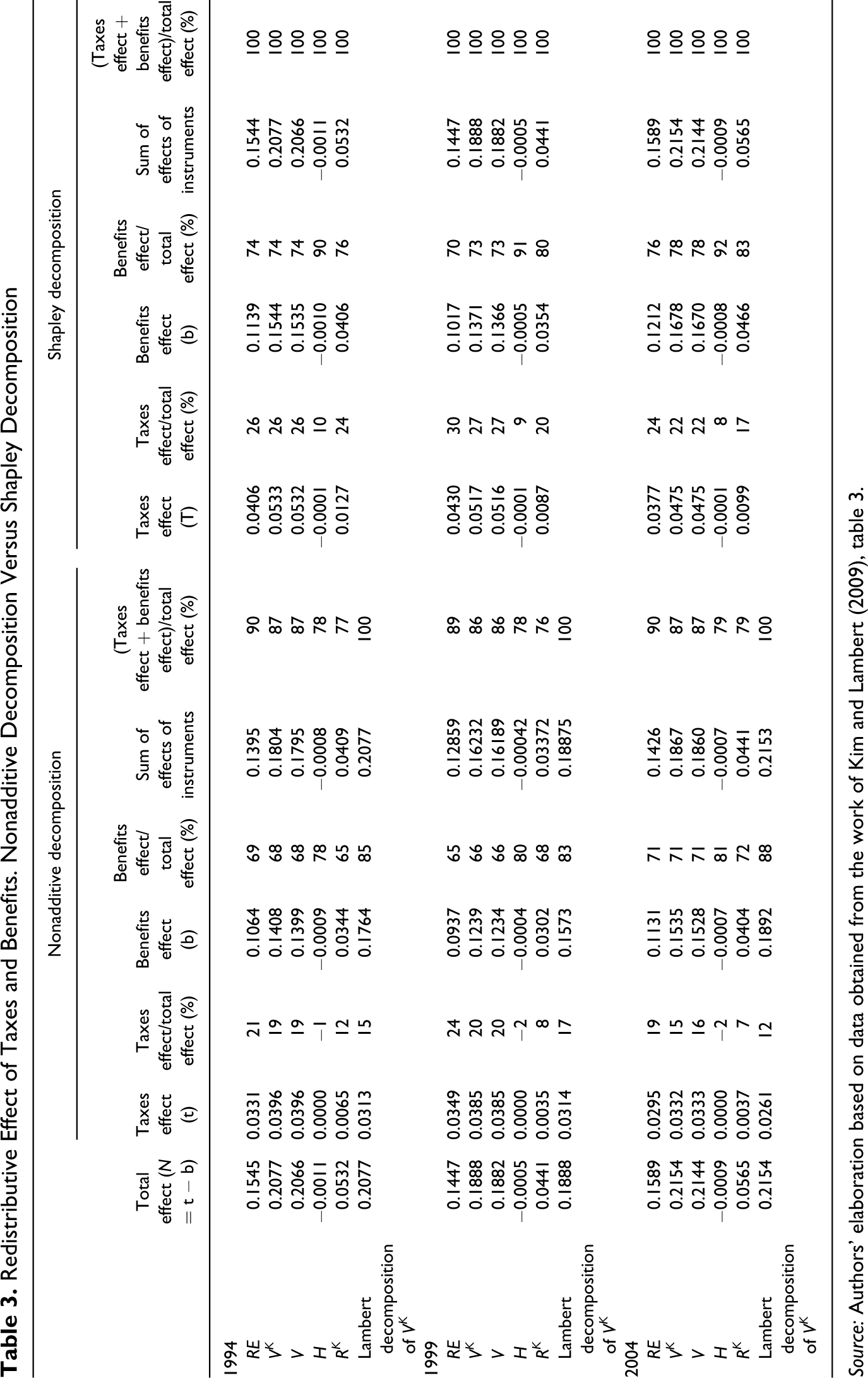
Source: Authors' elaboration based on data obtained from the work of Kim and Lambert (2009), Table 3.

Table 4.

Nonadditive Decomposition versus Shapley Decomposition, Difference in Percentage, 2004

	Taxes (a)			Benefits (b)
	Nonadditive decomposition (I)	Shapley methodology (II)	Difference in percentage ((I–II)/II)	Nonadditive decomposition (I)	Shapley methodology (II)	Difference in percentage ((I–II)/II)
RE	0.02954	0.03766	−21.56%	0.11307	0.12119	−6.70%
V^K	0.03323	0.04754	−30.10%	0.1535	0.16781	−8.53%
V	0.03326	0.04747	−29.93%	0.15276	0.16697	−8.51%
H	0.00002	−0.00008	−126.67%	−0.00074	−0.00084	−11.38%
R^K	0.00369	0.00988	−62.65%	0.04043	0.04662	−13.28%
	Taxes and Benefits (c)			(a) + (b) − (c)
	Nonadditive decomposition (I)	Shapley methodology (II)	Difference in percentage ((I–II)/II)	Nonadditive decomposition	Shapley methodology
RE	0.15885	0.15885	0.00%	−0.01624	0
V^K	0.21535	0.21535	0.00%	−0.02862	0
V	0.21444	0.21444	0.00%	−0.02842	0
H	−0.00091	−0.00091	0.00%	0.00019	0
R^K	0.0565	0.0565	0.00%	−0.01238	0

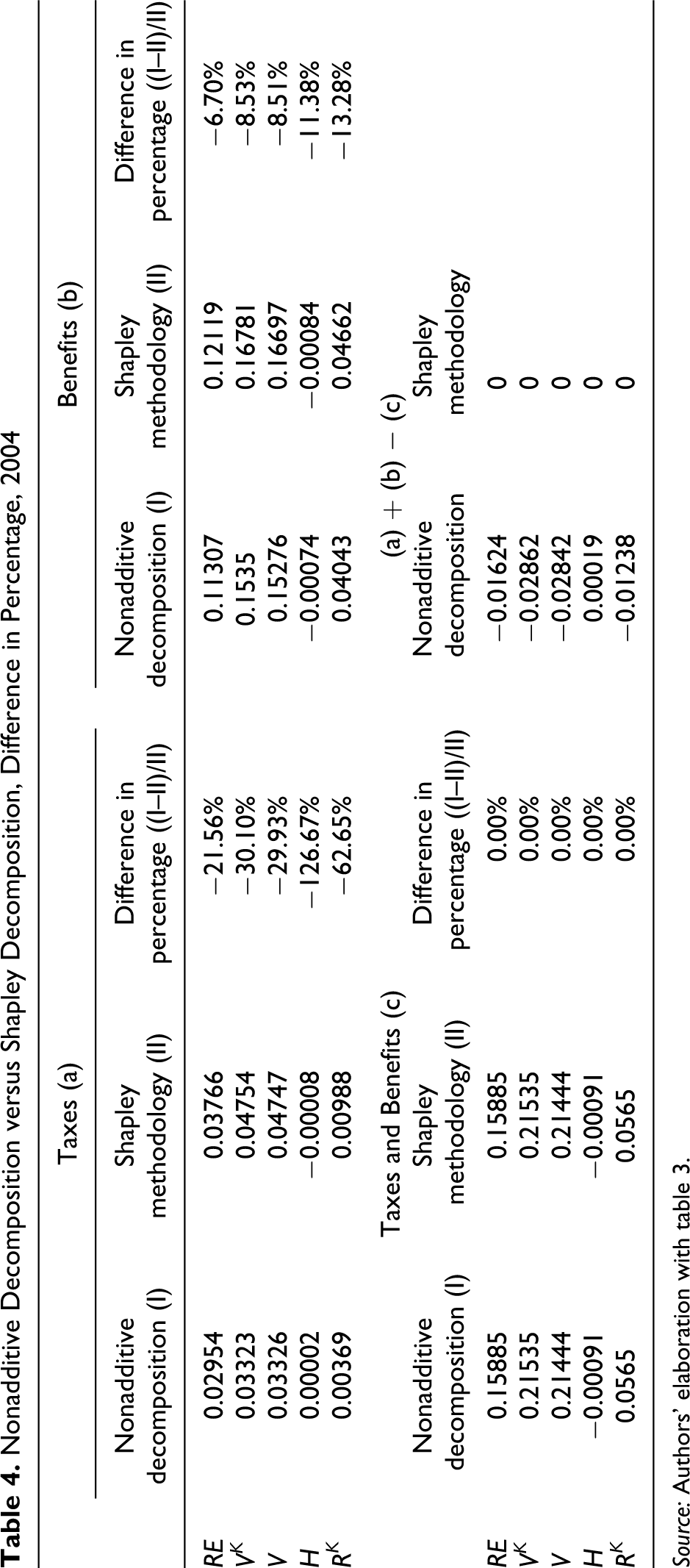
Source: Authors' elaboration with table 3.

In comparative terms, we observe that the redistributive effects of taxes and transfers separately are greater than those previously calculated and explain the whole redistributive effect. To explain this, we take taxes as an example and, using our methodology, we calculate the average of the two redistributive effects on the original income and on the income after benefits (I and III of Table 1). When taxes are applied after the benefits, these have already reduced the inequality and consequently with the same quantity of resources a greater equality can be attained. The most relevant effect for the taxes is that their redistributive effect is broader: they explain between 29.7 percent (1999) and 23.7 percent (2004) of the respective total effects. The new calculations also show a greater weight in the vertical effects of the taxes. This situation is coherent with its greater total redistributive effect.

It is also observed that, as Kim and Lambert (2009) pointed out, there is a certain stability of equality loss due to reranking, between 30 percent and 35 percent of the redistributive effect. Now, with the new calculations we also moreover identify the contribution of each instrument to the reranking. Thus, in 1994, 76 percent of the reranking was produced by transfers and 24 percent by taxes. In 2004, the taxes hardly contributed 17.5 percent of the reranking, which means that the transfers have a more unequal distribution in terms of horizontal equality.

Finally, we must highlight, also in the tax ambit, the sign change of the H values. In the original calculations, the taxes produced inequality as a consequence of an unequal treatment of equals. The new calculations point out that taxes and transfers follow a similar pattern. Inequality due to horizontal inequality is not produced, but rather this operates in favor of redistribution.

The previous information can be completed with that which appears in Table 4. This includes the relative variation in the calculations for 2004. We appreciate that the data of Kim and Lambert (2009) undervalued all the indices, but in comparative terms, the indicators of the redistributive effect of the taxes were more affected than those of the transfers. The undervaluing of the redistributive effect of the taxes triples that of the transfers. What is more, we can also see that the previous calculations undervalued the inequality associated with the horizontal inequality and the reranking more than the vertical redistributive effect.

To sum up, for the years analyzed, the result we obtain is that the redistributive effects of taxes and benefits are greater than those calculated on the initial income. At the same time, the calculations allow us to conclude that the undervaluing of the redistributive effect is greater in the case of the taxes. According to our estimation, the relative weight of the taxes would represent around 24 percent of the total redistribution, which contrasts with 12 percent attributed by Kim and Lambert for 2004, who use V^L instead of RE^HGA ; that is, the weight of the taxes in the redistribution in the United States for the years considered is notably greater when it is assessed taking into account the rest of the policy it is part of or with which it is associated. This is because, as Lambert (1985) states, when the taxes and/or transfers produce a reranking of the units of income, each term of the decomposition of V^L is a measure of the weight of the instrument in the progressivity but not in the redistributive effect.

Finally, with regard to the comparison of the values of V^L and V^HGA , given that we find ourselves in situation I of Table 2, in which taxes and transfers are progressive, it is fulfilled that for the taxes V^HGA > V^L and for the transfers V^HGA < V^L ; that is, the interaction of taxes and transfers increases the relative weight of the taxes in the vertical effect and reduces that of the transfers.

A Final Comment

Our main contribution is that we offer a decomposition of RE, V, H and R that consistently, symmetrically, and directly determines the individual contribution of taxes and benefits to the net budget; that is, the total effects are explained by the sum of the individual contributions, the decomposition is symmetrical because it does not depend on the aggregation ranking, and it is direct because each index can be calculated without the need to calculate the rest.

Applying Shapley value, we have managed to determine the contribution relative to the redistributive effect and its decomposition into the vertical and horizontal impacts of the instruments considered in Kim and Lambert (2009). We have consistently calculated the contribution of taxes and benefits to the total redistributive effect of the social well-being policies, and also the contribution to the vertical, horizontal, and reranking effects.

Along with this, a relevant repercussion is that it reduces the effect of discretional decisions in the results. In Table 5 , we have reproduced Table 1, but with the values calculated in Table 4 for the redistributive effect of 2004. In it one can clearly appreciate the incidence of evaluating the effect of the instrument as if it were applied alone. Thus, if taxes and transfers are evaluated on the initial income (alternative of the boxes I and IV), exactly as we have seen in Table 3, the effects of taxes and transfers are undervalued. On the contrary, if taxes and transfers are evaluated on income post transfers or income post taxes, respectively (or take the opposite alternative, that defined by boxes II and III), then the effects of both are overvalued. In both cases, the interactions are not evaluated. On the other hand, if we choose sequential sequence 1 (initial income − taxes + transfers), the redistributive effect of the taxes is undervalued and that of the transfers is overvalued. Finally, if we choose sequence 2 (initial income + transfers − taxes), the opposite occurs: the overvaluing is produced in the value of the taxes. When we calculate RE^HGA, V^HGA, H^HGA , and R^HGA , what we do is to eliminate the need to select one of these alternatives, and by doing so we eliminate the bias that stems from discretionally selecting the income on which the redistributive effect of each instrument of the welfare policy is calculated.

Table 5.

Additive Decompositions. Redistributive Effect of Taxes and Benefits 2004.

	Sequence 1	Sequence 2	Shapley solution
	(−t + b)	(b − t)	Shapley solution
Taxes	0.02954	0.04578	0.03766
Taxes	(I)	(III)	(V)
Benefits	0.12931	0.11307	0.12119
Benefits	(II)	(IV)	(VI)
Total	0.15885	0.15885	0.15885
Total	(VII)	(VII)	(VII)

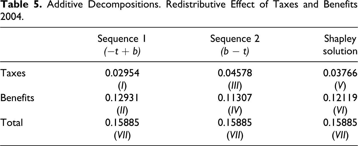
To sum up, applying Shapley value to the calculating of the redistributive effects provides accuracy, completes the information, and reduces the repercussions of discretionally choosing the sequence on which the redistributive effect is calculated. This methodology also appreciably improves the system used to decompose the redistributive effect of the net budget. Until now, the methodology most widely used, worked out by Lambert (1985), consists of decomposing only the vertical effect, V, thereby avoiding the horizontal effects. Moreover, Kim and Lambert (2009) offer two values of V—V^K and V^L —both for taxes and for benefits, to evaluate the vertical effect of taxes and benefits. With our methodology, we contribute a single value of the vertical effect of each instrument, and thereby the measurement carried out is not called into doubt.

This advantage does not avoid the need to analyze the origin of the discrepancy as both Lambert’s decomposition and ours offer additive results. From this analysis, we deduce that the difference is due to Lambert’s methodology not taking into account the interactions between the progressivity of taxes and benefits. This problem was clearly shown by Lambert (1985) himself and can be explained by our methodology. The interaction is evaluated by means of V^HGA , via the average of the weights relative to the instrument with respect to the income in each possible sequence (1 − t, or 1 + b, and 1 − t + b), instead of only with respect to the final relative income (1 − t + b), as in Lambert’s method. Furthermore, each instrument not only has a bearing on the vertical effect of the net budget via its own progressivity but also affects the vertical effect of the other instrument, by means of the change of the weighting of its progressivity.

To conclude, we point out that the additive and direct decomposition of the redistributive effect and its vertical and horizontal components allows the comparing of the relative weight of each instrument in percentage terms, and thereby improves the information of any comparative study not only in the case of intertemporal comparison but also for the comparing of policies or tax systems of different countries and for the comparing of alternatives in the composition of the net budget. This means that achieving a solution such as that proposed by us here merits consideration for future applied studies that include redistributive effects.

Footnotes

Luis A. Hierro, Rosario Gómez-Alvarez, and Pedro Atienza have examined the redistributive effects of intergovernmental grants in recent articles.

The author(s) declared no potential conflicts of interest with respect to the research, authorship, and/or publication of this article.

The author(s) received no financial support for the research, authorship, and/or publication of this article.

Notes

References

Aronson

Richard

Johnson

Paul

Lambert

Peter

. 1994. “Redistributive Effect and Unequal Income Tax Treatment.” Economic Journal 104:262–70.

Atkinson

Anthony

. 2004. “Increased Income Inequality in OECD Countries and the Redistributive Impact of the Government Budget.” In Inequality, Growth, and Poverty in an Era of Liberalization and Globalization, edited by Cornia

Giovanni Andrea

, 221–48. Oxford, UK: Oxford University Press.

Bibi

Sami

Duclos

Jean Yves

. 2010. “A Comparision of the Poverty Impact of Transfers, Taxes and Market Income Across Five OECD Countries.” Bulletin of Economic Research 62:387–406.

Deustch

Joseph

Silber

Jacques

. 2008. “On the Shapley Value and the Decomposition of Inequality Population Subgroups with Special Emphasis on the Gini Index.” In Advances on Income Inequality and Concentration Measures, edited by Betti

Gianni

Betty

Achille Lemmi

, 191–78. New York: Routledge.

Duclos

Jean-Yves

. 1993. “Progressivity, Redistribution and Equity, with Application to the British Tax and Benefit System.” Public Finance / Finances Publiques 48:350–65.

Garfinkel

Irwin

Rainwater

Lee

Smeeding

Timothy

. 2006. “A Re-examination of Welfare States and Inequality in Rich Nations.” Journal of Policy Analysis and Management 25:897–919.

Immervoll

Herwing

Levy

Horacio

Lietz

Christine

Mantovani

Daniele

O’Donoghue

Cathal

Sutherland

Holly

Verbist

Gerlinde

. 2005. “Household Incomes and Redistribution in the European Union, Quantifying the Equalising Properties of Taxes and Benefits.” IZA Discussion Papers 1824, Institute for the Study of Labor, Bonn.

Jenkins

Stephen P.

1988. “Reranking and the Analysis of Income Redistribution.” Scottish Journal of Political Economy 35:65–76.

Kakwani

Nanak

. 1984. “On Measurement of Taxes, Progressivity and Redistributive Effect of Taxes with Applications to Horizontal and Vertical Equity.” Advances in Econometrics 3:149–68.

10.

Kim

Kinam

Lambert

Peter J.

. 2009. “Redistributive Effect of U.S. Taxes and Public Transfers, 1994-2004.” Public Finance Review 37:3–26.

11.

Kolenikov

Stanislav

Shorrocks

Anthony

. 2005. “A Decomposition Analysis of Regional Poverty in Russia.” Review of Development Economics 9:25–46.

12.

Lambert

Peter J.

1985. “On the Redistributive Effect of Taxes and Benefits.” Scottish Journal of Political Economy 32:39–54.

13.

Lerman

Robert

Yitzhaki

Shlomo

. 1995. “Changing Ranks and the Inequality Impacts of Taxes and Transfers.” National Tax Journal 48:45–59.

14.

Reynolds

Morgan

Smolensky

Eugene

. 1977. Public Expenditure, Taxes and the Distribution of Income, The United States 1950, 1961, 1970. New York: Academic Press.

15.

Shapley

Lloyd S.

1953. “A value for N-person Games.” In Contributions to the Theory of Games II, edited by Kuhn

H. W.

Tucker

A. W

, 307–17. Princeton, NJ: Princeton University Press.

16.

Shorrocks

Anthony F.

1999. “Decomposition Procedures for Distributional Analysis: A Unified Framework Based on the Shapley Value.” Unpublished paper, University of Essex, Colchester, UK.

17.

Smeeding

Timothy M.

2005. “Public Policy, Economic Inequality, and Poverty: The United States in Comparative Perspective.” Social Science Quarterly 86:955–83.

18.

Urban

Ivica

. 2010. “Decomposing Redistributive and Reranking Effects to Reveal Contributions of Taxes and Benefits.” Institute of Public Finance working paper, Zagreb, Croatia.

19.

Urban

Ivica

Lambert

Peter J.

. 2008. “Redistribution, Horizontal Inequity and Reranking: How to Measure them Properly.” Public Finance Review 36:563–87.

20.

Wolff

Edward N.

Zacharias

Ajit

. 2007. “The Distributional Consequences of Government Spending and Taxation in the U.S., 1989 and 2000.” Review of Income and Wealth 53:692–715.