Bribe-Switching

Abstract

The US Foreign Corrupt Practices Act (FCPA) prohibits the payment of bribes to foreign public officials. We uncover an unintended consequence—the shadow economies of the countries of these officials increase after FCPA enforcement. Our hypothesis is that corrupt officials may be switching to taking bribes from illegal markets. We find that one case of FCPA enforcement alone increases the shadow economy by as much as 0.27 percentage points (pp), tree loss—an indicator of illegal logging—by 0.027 pp, and trade misinvoicing by 0.5 pp. Our results suggest the need to harmonize anti-corruption policies across all sectors—legal and illegal.

Keywords

corruption bribery shadow economy illegal markets

Introduction

The US Foreign Corrupt Practices Act (FCPA) is one of the most important pieces of anti-corruption legislation in the world. It prohibits US firms and persons, and foreign entities that have any dealings with the US, from paying bribes to foreign public officials. It is the FCPA that enabled the US Department of Justice (DOJ) and the Securities and Exchange Commission (SEC) to prosecute Goldman Sachs for its involvement in the Malaysian 1MDB corruption scheme, and Petroleo Brasileiro SA for the Petrobras bribery scandal in Latin America, two of the biggest corruption cases of all time. The DOJ and SEC imposed penalties of 3.3 billion dollars against Goldman Sachs and 1.78 billion against Petroleo Brasileiro (Cassin 2018, 2020). Since the FCPA's inception in 1977, many other large companies have been prosecuted and fined for at least 100 million dollars, including General Electric, KBR/Halliburton, Alstom, Ericsson, and Siemens. Between 1977 and 2019, over 580 corruption cases have been filed with nearly $17 billion in fines imposed.¹

While the FCPA was originally designed to prosecute corrupt US-based companies that operate internationally, its scope greatly expanded in 1998. The 1998 amendment widened FCPA jurisdiction to include any domestic or foreign entity (firm or individual) that engages in a corrupt act which involves the US in any way. This includes, for instance, using US email servers and the US banking system to facilitate corrupt transactions, and holding meetings in any US territory during which corrupt deals are discussed. FCPA enforcement against US and non-US entities has been so far-reaching that Christensen et al. (2022) refer to FCPA enforcers as “policeman for the world.”

Notwithstanding the rapid increase of FCPA enforcement and FCPA-related anti-corruption efforts around the world, still little is known about its impact on economies. How does the FCPA affect the countries of the foreign public officials that receive bribes? Is FCPA enforcement good for their economy?

Yes—for their shadow economy, that is. We demonstrate in this paper that after a FCPA case is filed against an entity that has paid bribes to foreign officials, the latter country's shadow economy as a percentage of GDP rises by as much as 0.27 percentage points (pp), or approximately $540 million a year.

Our hypothesis is that when corrupt public officials extract bribes from both legal and illegal markets, greater anti-corruption efforts in one market induces officials to switch their bribe-taking to the other. FCPA enforcement raises public officials’ cost of bribe-taking from legal markets, relative to the cost of bribe-taking from illegal markets. This prompts officials to extract less bribes from legal entities and more from illegal ones, in exchange for “allowing” more illegal production. In equilibrium, the size of illegal markets increases.

To test this bribe-switching hypothesis, we first estimate the effect of an FCPA case on the GDP per capita of the country whose officials are party to the case, as well as the effect on each of the expenditure components—consumption, investment, government expenditure, exports, and imports. We find that among countries with relatively low initial levels of corruption, GDP per capita and all components decrease. Among countries with higher initial levels of corruption, investment, exports, and imports go down, while GDP per capita is unchanged.

If FCPA enforcement increases the cost of, and therefore deters officials from extracting bribes from, e.g., investment contracts, it would thus lessen the incentive of corrupt officials to approve such contracts. This, then, would decrease investment. That we find that investment falls after FCPA enforcement suggests that bribe-rents have also fallen; more so since we find a larger drop in countries with higher initial levels of corruption.²

However, even if some bribe-rents have decreased, it does not necessarily follow that total rents have fallen. In fact, we find no evidence that corruption scores improve after FCPA enforcement. Note also that while investment has decreased across all countries, only the low-corruption countries have experienced a drop in GDP per capita—GDP per capita in the high-corruption countries remains the same. This suggests that in the latter, corrupt public officials might be recovering lost bribe-rents from investment by extracting rents from other sources.

Where can corrupt public officials extract other rents to recoup lost ones? It is plausible that the wide scope of FCPA enforcement could deter corruption in many markets by making bribe-taking from many kinds of transactions more costly. Arguably, however, its deterrent effect on corruption in illegal markets would be smaller, if any. By their nature, illegal markets are hidden. Uncovering corruption in these markets is much more difficult since it requires piercing an already formidable veil of secrecy. In contrast, transactions in legal markets are relatively more transparent, making it less difficult to investigate whether such transactions violate the FCPA.

If FCPA enforcement has a greater corruption deterrent effect in legal, than in illegal, markets, then a public official who takes bribes from both markets would be induced to switch some of its bribe-taking to illegal markets. This would then cause illegal markets to grow. Note that the bribe-switching and growth in illegal markets should be more likely in countries in which public officials are already taking bribes from both legal and illegal markets. It would be easier to extract more bribes, than to start extracting bribes, from illegal markets when bribe-taking from legal markets becomes more costly.

Our primary proxy for the size of illegal markets is the size of the shadow economy as a percentage of GDP, constructed by Medina and Schneider (2019). To distinguish countries whose public officials are already likely taking bribes from both legal and illegal markets, we split our sample according to the initial levels of corruption, as well as the initial size of the shadow economy. Bribe-switching should be more apparent in countries where corruption is initially high and the shadow economy initially large.

As alternative indicators of illegal markets, we also look at homicide rates, tree loss (an indicator of illegal logging), and trade misinvoicing. A common way to misinvoice trade is to underreport imports in order to avoid paying import taxes. Trade misinvoicing thus depresses the (reported) value of imports. It is telling that imports of highly corrupt countries decrease after FCPA enforcement, while their investment and exports fall, thereby keeping their GDP per capita unchanged. We find that after FCPA enforcement, shadow economies, homicide rates, and trade misinvoicing all go up, with the effects being more pronounced for countries that initially have higher corruption and larger shadow economies.

The paper makes several contributions to the anti-corruption literature. First, we demonstrate that anti-corruption efforts, when focused only on certain kinds of transactions, can induce corrupt public officials to switch to other sources of rents (Olken and Pande 2012). Olken (2007) finds that in Indonesia, the auditing of road projects decreased leakages, but increased nepotism, as officials ended up hiring up more relatives to work on the roads. Desierto (2021) shows that municipal mayors in the Philippines decrease bribe-taking when they can get more rents from appropriating government revenues. Burgess et al. (2012) provides evidence of rent–switching between oil and gas rents and illegal logging in Indonesia. Arbatskaya and Mialon (2020) provide a model of switching of investment contracts from US firms to foreign competitors when the FCPA is enforced only against the former.

Second, we add to a small but growing literature on the economic analysis of the FCPA. Arbatskaya and Mialon (2020) formally analyze bribery and investment activities of firms that are subject to FCPA enforcement. With the recent exception of Christensen et al. (2022), which shows that FDI in high-corruption countries fall after FCPA enforcement, empirical papers have mostly focused on the effect of the FCPA on US firms and their competitiveness—Graham and Stroup (2016), Lippitt (2013), Wei (2000), and Hines (1995) are examples. Our paper, in contrast, analyzes the effect of the FCPA on the foreign country whose public officials are recipients of the bribes. Causal identification is possible to the extent that foreign public officials have no control over the DOJ or SEC's decision to initiate a case against entities that have paid bribes to those officials. We exploit the fact that bribery is two-sided—the bribe offer by the entity has to be accepted by the foreign public official before bribes can actually be paid. Thus, FCPA enforcement against the entity exogenously triggers a decrease in bribe extraction by the foreign public official.

Lastly, the paper contributes to the nascent debate on whether corruption and the shadow economy are complements or substitutes. (See Borlea et al. (2017) for a review.) Johnson et al. (1998), Choi and Thum (2005), and Dreher and Siemers (2009) posit that firms go underground to avoid government-induced distortions, e.g., bribe-taking. The implication is that as the latter becomes more ubiquitous, then the shadow economy increases as more firms go underground to avoid having to pay bribes. Illegal production thus substitutes for the corrupt transaction in legal markets. On the other hand, corruption and the shadow economy can be complements if illegal producers pay bribes to avoid getting caught (Dreher et al. 2009; El-Shagi 2005; Hindriks et al. 1999). Combining both strands, Dreher and Schneider (2010) posit that in low-income countries, firms pay bribes to operate in the shadow economy—“underground activities require bribes and corruption,” whereas in high-income countries, they pay to obtain large contracts in the legal sector. The authors thus suggest that corruption and the shadow economy are complements in low-income countries, but substitutes in high-income countries, and provide some evidence for this. Using cross-sectional data on 98 countries, they show that among the low-income countries, an increase in corruption perceptions is associated with an increase in the shadow economy, while there is no such association among high-income countries.

In our paper, we allow for the possibility that bribery can take place both in legal and illegal markets. An increase in the expected costs of bribery in legal markets, e.g., due to FCPA enforcement, makes bribe-taking relatively easier in illegal markets, inducing corrupt officials to switch some of their bribe extraction to the latter. In exchange for paying more bribes, illegal producers are “allowed” to increase production, and the shadow economy grows. We provide evidence using the most exhaustive panel of countries ever assembled to analyze the effect of the FCPA. Using a difference-in-differences (DID) framework, we employ the de Chaisemartin and D’Haultfœuille (2023) estimator to accommodate heterogeneous treatment effects, as FCPA cases are filed at different time periods.³ This also allows us to adopt a dynamic DID model and estimate pre-treatment placebo parameters, and to include a country-specific linear time trend. For robustness, we also generate results using the DID estimators of Callaway and Sant’Anna (2021) and Cengiz et al. (2019). These latter results are similar and are relegated to an Online Appendix.

The rest of the paper is organized as follows. Section “Data” motivates our outcomes of interest (via a conceptual model) and describes the data. Section “Empirical Strategy” discusses the identification strategy and empirical estimator. Section “Results on Economic Activity after FCPA Enforcement” estimates the effect of FCPA enforcement on GDP per capita, its expenditure components, and corruption scores, while Section “Results on Illegal Markets” presents the main results—the effect of enforcement on the shadow economy and other proxies for illegal markets. Section “Conclusion” concludes.

Data

Our primary hypothesis is that FCPA enforcement leads to bribe-switching from legal to illegal markets in foreign countries. Given the difficulty in measuring both corruption and illegal activity, introducing the data necessary to test this hypothesis is not as simple as describing measures of corruption in legal versus illegal markets as these measures do not presently exist. First, we discuss and motivate our choice of outcomes (GDP per-capita, corruption perceptions, GDP per-capita components, and various measures illegal activity) via a conceptual model and in doing so, we also describe the FCPA in further detail. This is done in the Section “Conceptual Framework and Outcome Variables.” Second, before delving into identification and specific empirical estimators, it is important to understand the frequency of FCPA cases through time (i.e., the treatment) and the sample of countries directly affected by FCPA enforcement (i.e., our treatment group). We do this in the Section “Treatment Variable and Sample.” We reserve discussions of our empirical strategy and estimator for the Section “Empirical Strategy.”

Conceptual Framework and Outcome Variables

The FCPA was signed into law in 1977 and was first enforced by the SEC and DOJ in 1978. The anti-bribery provisions of the law prohibit US persons, entities, and certain foreign issuers of securities from making illicit payments to a foreign official in exchange for obtaining or retaining business.⁴ The law was then amended in 1998 to implement the requirements of the OECD Anti-Bribery Convention that signatories outlaw bribe payments to foreign officials. Specifically, this amendment makes the anti-bribery provisions also apply to foreign persons and entities that act in furtherance of illicit payments within the territory of the United States. Such actions include:

“…placing a telephone call or sending an e-mail, text message, or fax form, to, or through the United States involves interstate commerce–as does sending a wire transfer from or to a U.S. bank or otherwise using the U.S. banking system, or traveling across state borders or internationally to or from the United States (pg. 10, FCPA Resource Guide, 2015).”

We focus on the effect of FCPA enforcement following this 1998 amendment. Compared to the original law, the amended version, with its wider scope, has greater potential to deter corruption in foreign countries, which comprise our population of interest. Deterrence can occur through direct or indirect ways. The FCPA can be directly enforced against foreign officials if they engage in corrupt activity through US channels. An example is Heon-Cheol Chi who was the Director of the Earthquake Research Center at the Korea Institute of Geoscience and Mineral Resources. The DOJ was able to indict him for laundering bribe-money through the Bank of America.

Indirectly, FCPA enforcement can trigger anti-corruption efforts in foreign countries whenever the US shares information with local authorities. In fact, the US and other signatory countries to the 1997 OECD Anti-Bribery Convention are obliged to provide mutual legal assistance and evidence sharing (Brewster 2017). Note, then, how large corruption scandals usually involve investigations and prosecutions in multiple jurisdictions—e.g., scandals involving Siemens, Technip, Halliburton, BAE systems (Brewster 2017) and, of course, 1MDB and Petrobras.⁵ The Convention also aims that, with the example of the FCPA, other countries will also institutionalize their own anti-corruption efforts by, e.g., outlawing bribery.

Thus, by exposing corrupt transactions involving foreign public officials, FCPA enforcement can prompt host countries to conduct their own investigations or, in some cases, let the US directly prosecute the foreign officials. Regardless, enforcement leads to an increased cost of bribe-taking in legal markets. On the one hand, this could reduce bribe-taking by foreign public officials. In turn, lower corruption in their countries can lead to higher growth (Gründler and Potrafke 2019; Mauro 1995; Mo 2001), investment (Cieślik and Goczek 2018; Zakharov 2019), and entrepreneurship (Bologna and Ross 2015; Colonnelli and Prem 2022; Dutta and Sobel 2016).

However, since FCPA enforcement is focused on anti-corruption in legal markets, it could alternatively lead to a reallocation of corruption from the legal to the illegal sector. Both effects are consistent with an elevated cost of bribe-taking in legal markets, however the latter does not suggest that FCPA enforcement would reduce corruption overall. Ultimately, the effect of FCPA enforcement on the foreign economy, then, is an empirical question.

Our central hypothesis is that that FCPA enforcement can induce bribe-switching from legal to illegal markets. If corrupt public officials take bribes from both legal enterprises (e.g., by awarding formal contracts) and illegal producers (e.g., to avoid taxation) then an increase in the cost of taking bribes from legal markets can induce officials to decrease their bribe-taking from legal markets and increase it from illegal markets. To extract larger bribes from the latter, public officials enforce less against illegal producers—à la Becker et al. (2006) and Desierto and Nye (2017)—thereby increasing the size of illegal markets. As discussed in the “Introduction” section, this is likely easier to do in countries that have already established, large illegal sectors. However, these are also the countries that have the most to gain from anti-corruption efforts yet are plausibly the ones least likely to engage in true anti-corruption reform. Because of these differing effects across groups, we study the impact of FCPA enforcement on initially highly corrupt versus (comparatively) non-corrupt countries separately.⁶ Our main focus is on the former; we use the latter as a falsification test.

If corruption is being reallocated, it is unlikely that aggregate economic activity changes as total corrupt activity is unchanged in response to FCPA enforcement. As such, the first two outcomes that we study are the country's overall level of GDP per-capita and corruption score. We measure GDP per-capita using the Penn World Tables (PWT) Version 9.1's measure of expenditure side real per-capita GDP. Corruption perceptions come from two alternative sources: the World Bank's Control of Corruption index and the International Country Risk Guide's measure of corruption risk. The former corruption measure is much more expansive in country coverage but is only available from 1996 onwards (and for the first several years, available only every 2 years). The latter has a smaller country coverage but is available for a longer time series (annually since 1984).

We then examine how FCPA enforcement impacts each major component of GDP per-capita (consumption, investment, government expenditures, exports, and imports). Because our goal is to understand how FCPA enforcement impacts illegal activity, understanding the dynamics of the changes in the specific GDP components is informative in this regard. While it might be expected that investment falls—either due to a reduction in investment coming from the US specifically⁷ or in general as in Christensen et al. (2022)⁸—the simultaneous patterns uncovered in the other components can show off-setting effects that are consistent with both elevated illegal activity and unchanging total productivity (i.e., GDP per-capita). For example, the impact of FCPA enforcement on trade—specifically imports—is informative as the underreporting of imports is a common way for illegal producers to conceal economic activity. This would have the effect of offsetting the reduction in investment in aggregate GDP per-capita measurements. Alternatively, it could be that government spending is elevated in an attempt to compensate for the loss of private investment spending. Like aggregate GDP per-capita, our measures of GDP per-capita components are derived from the PWT Version 9.1.

Lastly, we test the effect of FCPA enforcement on the size of the illegal markets more directly using a variety of estimates provided in the literature. The first is the most comprehensive in both country and time coverage and comes from Medina and Schneider (2019). This is a measure of “illegal activities (and) unreported income from the production of legal goods and services, either from monetary or barter transactions.”⁹ It is derived from a modified multiple indicator-multiple causes (MIMIC) model and a major criticism of this is that they use official GDP per-capita and GDP per-capita growth estimates as cause and indicator variables. They address these concerns through the use of satellite data on night light intensity in place of official GDP finding little change in their estimates. They also compare their estimates with a discrepancy-based measure of informality (specifically, the discrepancy between national expenditure and income statistics)¹⁰ finding that their estimates of shadow economic activity are robust to what this alternative measure would predict.

Nevertheless, given that this measure has concerns and that the shadow economy includes unreported incomes from legal production, we also estimate the effect of FCPA enforcement on other, more direct, indicators of illegal activities, viz., trade misinvoicing (an example of which is the underreporting of imports to avoid customs), homicide rates (per 100,000 people), and tree loss coverage (potentially due to illegal logging and mining). Trade misinvoicing is measured as the value gap (reported versus actual) as a percentage of total trade and comes from Global Financial Integrity. Homicide rates come from the United Nations Office on Drugs and Crime. Lastly, tree loss is measured as a percentage of total hectares and comes from the World Resources Institute's Global Forest Watch. Given the secretive nature of illegal activity, these estimates are sometimes sparse and can be imprecise. We present and discuss these results after examining the above discussed outcomes (GDP per-capita, corruption perception scores, and GDP per-capita components). To test the hypothesis that illegal activity is increasing following FCPA enforcement, it is necessary to examine the complete picture across all outcomes summarized in this conceptual model. This is also another reason why we limit our analysis to looking at only the effects of FCPA post-1998. The primary reason is that FCPA enforcement post-1998 is fundamentally different and more focused on foreign entities, thereby more likely to affect their economies. However, a secondary reason is that most data concerning corruption and illegal activity is not available prior to 1990.

To summarize, FCPA enforcement is likely to increase the cost of bribery in legal markets. If FCPA enforcement encourages bribe-switching to illegal markets and does not effectively reduce corruption as hypothesized, we should see minimal changes in overall economic activity and corruption perception scores. We should also see simultaneous changes in individual GDP per-capita components consistent with this story. Lastly, even if imprecise, our explicit illegal market indicators should show some growth following FCPA enforcement. We view these results, collectively, as a test as to whether FCPA enforcement induces bribe-switching, especially in initially high corruption and/or largely informal countries.

Table 1 lists the outcome variables we use; Table 2 lists the associated summary statistics. The next section describes the treatment variable and sample.

Table 1.

Variable Names, Brief Descriptions, and Sources for Dependent Variables.

Name	Brief description	First available year^a
Economic Output
Real GDP per-capita	Expenditure Side Real GDP per-capita (PWT)^b	1978
Economic Components
Consumption	Real consumption per-capita (PWT)	1978
Investment	Real investment per-capita (PWT)	1978
Government	Real government per-capita (PWT)	1978
Exports	Real exports per-capita (PWT)	1978
Imports	Real imports per-capita (PWT)	1978
Corruption Reform
World Bank Corruption	Cor. index with a scale of −2.5 (most corrupt) to 2.5 (least corrupt) (WBG)	1996
ICRG Corruption	Cor. index with a scale of 1 (most) to 6 (least) (ICRG)	1984
Illegal Activity
Shadow Economy	Shadow economy as a % of official GDP (MS)	1991
Other Illicit Activities
Homicide Rate	Homicides per 100,000 people (UNODC)	1990
Tree Loss	Tree loss as a % of total hectares (GFW – WRI)	2000
Trade Misinvoicing	Value gap in trade as a % of total trade (GFI)	2008

First available year relative to the 1978 start date of the FCPA program.

Sources: (1) PWT—Penn World Tables Version 9.1. (2) MS—Medina and Schneider (2019). (3) WBG—World Bank Governance Indicators. (4) ICRG—International Country Risk Guide. (5) UNODC—United Nations Office on Drugs and Crime. (6) Global Forest Watch—World Resources Institute. (7) Global Financial Integrity.

Table 2.

Summary Statistics for Dependent Variables.

Name	Obs.	Mean	St. Dev.	Min	Max
Economic Output
Real GDP per-capita	4,982	14,998	17,270	223	153,458
Economic Components
Consumption	4,926	7,983	8,925	166	224,619
Investment	4,926	4,050	6,370	8.766	183,765
Government	4,926	2,759	3,569	12.738	96,165
Exports	4,926	6,774	13,859	0.054	140,354
Imports	4,926	7,703	17,032	0.267	522,304
Corruption Reform
World Bank Corruption	4,406	−0.025	0.999	−1.869	2.470
ICRG Corruption	3,637	2.871	1.290	0	6
Illegal Activity
Shadow Economy	4,212	31.122	12.751	5.1	70.5
Other Illicit Activity
Homicide Rates	3,965	8.027	12.226	0.000	141.723
Tree Loss	2,907	0.181	0.289	0.000	3.287
Trade Misinvoicing	1,175	19.763	5.887	0.030	87.240

Notes: All per-capita variables (GDP and GDP components) and homicide rates enter regressions in logged form. All other dependent variables enter regressions in their raw form.

Treatment Variable and Sample

We use data on FCPA enforcement cases compiled by the FCPA Clearinghouse at Stanford Law School. To focus on the effect of the 1998 reform, and to maximize the number of observations for which data are available, we consider 1990 through 2019 as our sample period.¹¹ For each case, information is provided on the identity of the US person or entity against which the case is filed, the date in which the case was initiated, the prosecuting agency (SEC or DOJ), the amount of the bribe paid, the country in which it was paid, and the amount of the sanction or settlement. Since we can calculate, for each country in each year of the sample, the number of FCPA cases involving that country, we are able to form a country-year panel of FCPA cases.

Prior to 1998, there were only a total of 42 FCPA cases filed over a 20-year period. In addition, the size of the penalties (fines) in these early cases was comparatively small. As noted in Brewster (2017), even the tenth highest fine in more recent years (post-reform) is more than twice the combined penalties from the first two decades of the program. After the 1998 reform, the number of cases jumped—544 cases filed between 1998 and 2019. These include cases involving non-US firms that are covered by the 1998 amendment. In 2019, for instance, 8 out of the 14 enforcement cases filed against corporations were against foreign entities. The total amount of settlements from the 2010 cases alone was almost $3 billion US dollars, and about half of which are from the cases against foreign entities.¹²

We assign zero number of cases to the country from 1990 until the first year after 1998 (i.e., post amendment) that the country experiences its first FCPA enforcement case.¹³ For countries that never experienced FCPA enforcement, a zero is always assigned. FCPA enforcement, following 1998, affected many countries. Of the 219 countries in our sample, 113 experienced FCPA enforcement at some point between 1998 and 2019. Moreover, many countries also experienced subsequent enforcement after the first case is filed. Figure 1 summarizes this pattern. Time point 0 represents the country's first year of experiencing FCPA enforcement, which generates an average of 1.7 cases across all the countries in the treated group (i.e., the group of countries experiencing any FCPA enforcement).¹⁴ The number of cases grows thereafter.

Figure 1.

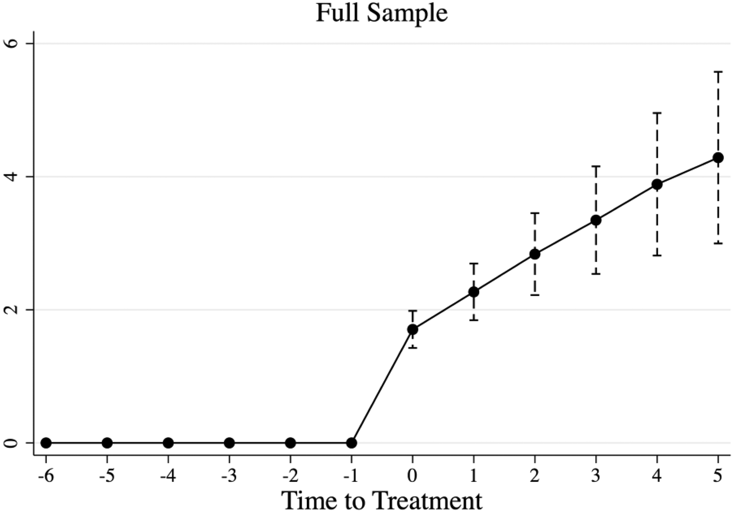
Cumulative sum of FCPA cases—full sample. Notes: Bars correspond to 95% confidence intervals. FCPA case data comes from the FCPA Clearinghouse at Stanford Law School.

Figure 2 splits the sample evenly according to the countries’ initial (pre-1998) corruption perception scores and shows that more cases are filed involving public officials in relatively more corrupt countries. This pattern can help allay concerns regarding potential biases of the SEC and DOJ. That is, if cases are filed based on merit, one would expect the SEC and DOJ to file more cases involving public officials in relatively more corrupt countries. To account for this difference, we also provide separate estimates for countries that have relatively higher, and those that have relatively lower, initial corruption perception scores.¹⁵ In addition, more corrupt countries to begin with are more likely to experience bribe-switching.

Figure 2.

Cumulative sum of FCPA cases—high-corruption versus low-corruption group.

The pattern of cases filed post-1998 suggests that being treated with FCPA enforcement is like experiencing changes in the treatment “dosage” over time. As de Chaisemartin and D’Haultfœuille (2023) discuss, this type of treatment can be extremely complicated to interpret. We thus follow their approach in defining the initial instance of enforcement as a binary treatment. Specifically, our treatment variable equals one in the year in which the first FCPA case was filed and remains one thereafter. After estimating the effect of this binary treatment variable, we then divide it by the yearly case count to get an estimate of the effect of a single FCPA case.¹⁶

Empirical Strategy

To test whether the FCPA enforcement has an effect on our various outcome variables (described in Section 2.1 and summarized in Table 1), we use the dynamic difference-in-difference estimator with country specific linear time trends as developed in de Chaisemartin and D’Haultfœuille (2023). As discussed in the preceding section, our treatment indicator is binary and becomes one in the first year of FCPA enforcement involving country i and remains one thereafter. We estimate both pre-treatment (i.e., placebo) and post-treatment dynamic effects by including up to 5 years of lags and leads of this treatment indicator. Specifically, we denote the indicator as ${FCPA}_{i t}^{d}$ , where d indicates the period relative to the first year of FCPA enforcement. It is defined as d = {l, l + 1, l + 2, … 0, 1, 2, …, L}, with l = −5 and L = 5. Thus, d = −1 is the first year prior to country i's first FCPA enforcement case; d = 0 is the year of first enforcement, d = 5 after 5 years, and so on.

We adopt a dynamic specification to allow for the possibility that the treatment generates different effects over time:

Y_{i t} = \sum_{d = l}^{L} α_{d} {FCPA}_{i t}^{d} + μ_{t} + η_{i} + β_{i} γ_{i t} + u_{i t},

(1)

where µ_t are year fixed effects, η_i country fixed effects, γ_it is a country-specific time trend, and u_it is the error term. Standard errors are clustered by country and calculated using 250 bootstrap replications. One could estimate (1) using OLS, but this can yield biased estimates if there are heterogeneous treatment effects. De Chaisemartin and D’Haultfœuille (2020, 2023) have shown that OLS regression of two-way fixed effects models (TWFE) with binary or non-binary treatments estimates the weighted average of the treatment effects across groups, where the weights can be negative. This can then yield estimates that are opposite of their true sign.

More generally, treatment heterogeneity raises the primary issue of whether the control units are appropriate. We have 219 countries in our full sample with 113 experiencing an FCPA treatment at some point. Even with 106 never treated (control) countries, however, typical TWFE models use previously treated units and never treated units as controls for newly treated units when the treatment is staggered through time. This can be problematic if treatment effects are heterogenous across time or across treatment groups. Indeed, many new estimators have been proposed to address this problem. The de Chaisemartin and D’Haultfœuille (2023) estimator, for instance, uses both never-treated and not-yet treated units as controls. Already-treated units are never used as controls. The Callaway and Sant’Anna (2021) estimator uses only never-treated units as controls. Another estimator that uses only never-treated units as controls is the stacked difference-in-difference approach à la Cengiz et al. (2019). The key similarity across all estimators is that already treated units do not serve as controls. de Chaisemartin and D’Haultfœuille (2022) provide a summary of these new estimators and their differences, as well as research in this area.

We rely on the de Chaisemartin and D’Haultfœuille (2023) estimator as it can accommodate country specific linear time trends which are apparent in our data.¹⁷ We also estimate all results using this same estimator without a linear time trend, using the alternative Callaway and Sant’Anna (2021) and Cengiz et al. (2019) estimators, and using OLS as a comparison. These robustness checks yield similar estimates and are relegated to an Online Appendix.

We implement the de Chaisemartin and D’Haultfœuille (2023) estimator in STATA using the did_multiplegt module. This yields output analogous to an event study design where the placebo option estimates parameters {α_d}, d < 0, while the dynamic option estimates dynamic treatment effects {α_d}, d ≥ 0. In both cases, the coefficients are to be interpreted as long-run differences between the period in question and the placebo period immediately prior to the treatment (Roth 2024). Thus, for all cases, the period d = −1 will have a coefficient equal to zero by definition (i.e., this is the reference year). Each estimated treatment effect can then be assessed relative to this placebo period.

Recall that a complexity of our treatment is that the actual number of cases, and therefore treatment intensity, can vary across treated units. De Chaisemartin and D’Haultfœuille (2023) recommend normalizing the estimated treatment effect by the number of cases. That is, by dividing parameter estimates by the average number of cases in the appropriate year post-treatment, one can obtain the effect of an additional FCPA case. For example, as shown in Figure 1, the typical treated country experiences 1.7 cases in time point 0 (the first instance of the treatment). Our treatment effects estimated in Equation (1) consider all enforcement activities, thus dividing this number by 1.7 would yield a per-case effect. Note that doing so does not separately identify the effect of the first case/s and the effects of the subsequent cases after the initial year. Normalizing only allows us to gauge whether the effect of a single case increases or decreases through time.

We also estimate the parameters separately for countries with high (HC) and low (LC) initial corruption perception scores. If countries in group HC have more widespread and endemic corruption, whereas those in group LC experience more isolated instances of corruption, it is then in group HC that corrupt officials are more likely to take bribes both from legal and illegal markets and, thus, more able to switch to more bribe-taking from the latter after FCPA enforcement. Comparing high corruption and low corruption countries, in this way, provides a falsification test for our hypothesis. Superscripting (1) by group, we then estimate:

Y_{i t}^{HC} = \sum_{d = l}^{L} α_{d}^{HC} {FCPA}_{i t}^{d HC} + μ_{t}^{HC} + η_{t}^{HC} + β_{t}^{HC} γ_{i t}^{HC} + u_{i t}^{HC},

(2)

Y_{i t}^{LC} = \sum_{d = l}^{L} α_{d}^{LC} {FCPA}_{i t}^{d LC} + μ_{t}^{LC} + η_{t}^{LC} + β_{t}^{LC} γ_{i t}^{LC} + u_{i t}^{LC} .

(3)

We expect

{\hat{α}}_{d}^{HC} = {\hat{α}}_{d}^{LC}

in the pre-treatment periods, that is, when d < 0, but that

{\hat{α}}_{d}^{HC} \neq {\hat{α}}_{d}^{LC}

in the post-treatment periods. Whether

{\hat{α}}_{d}^{HC}

is greater than or less than

{\hat{α}}_{d}^{LC}

post-treatment depends on the outcome of interest and implicit mechanism. Suppose Y is a measure of economic activity. If an FCPA case deters corrupt public officials from extracting bribes from legal markets, but they do not switch to taking bribes from illegal markets, then it might be that

{\hat{α}}_{d}^{LC} \geq {\hat{α}}_{d}^{HC}

in most, if not all, post-treatment periods (d ≥ 0). This is what would be expected if countries with lower corruption to begin with are more successful in conducting their own investigations and in pursuing other anti-corruption efforts that are spurred by FCPA enforcement. To further support this idea, one could then run regressions with Y as a measure of corruption. If better economic outcomes are due to successful anti-corruption efforts, then it must also be the case that

| {\hat{α}}_{d}^{LC} | \geq | {\hat{α}}_{d}^{HC} |

when d ≥ 0—i.e., FCPA enforcement subsequently lowers corruption in low corruption countries by at least as much as it does in high corruption countries.

On the other hand, if bribe-switching did occur between legal and illegal markets, it would be more likely in countries with widespread corruption, in which public officials are likely to obtain rents from multiple sources, including illegal producers who want to avoid detection and prosecution. In this case, one could also expect the effect on economic activity Y to be such that ${\hat{α}}_{d}^{LC} \geq {\hat{α}}_{d}^{HC}$ for most post-treatment periods. This is because public officials in low corruption countries might be more willing to substitute toward non-corrupt contracts/enterprises, whereas those in high corruption countries might be more able to preserve rents by switching their bribe extraction from legal, to illegal, sources. Necessary for this, however, is evidence that high corruption countries do not become less corrupt, as contrary evidence would suggest that their bribe-rents are not preserved. One could then estimate (2) and (3) with Y as indicators of illegal activities and show that ${\hat{α}}_{d}^{LC} < {\hat{α}}_{d}^{HC}$ when d ≥ 0, with ${\hat{α}}_{d}^{LC}$ possibly equal to zero if there were no bribe-switching in low corruption countries.

We conduct another, more direct, falsification test of our bribe-switching hypothesis by estimating (2) and (3) for countries that have, respectively, high and low initial size of illegal markets, as proxied by the initial (pre-1998) size of the shadow economy. Bribe-switching between legal and illegal markets should be more likely for countries that already have large illegal markets to begin with, irrespective of whether these countries have high or low initial corruption scores.

For both high corruption/low corruption and large shadow/small shadow comparisons, we provide separate estimates of the parameters and calculate a T-Statistic to test if the two estimates are statistically different from one another. We report the T-Statistic consistently as a one-sided test of the form: ${\hat{α}}_{d}^{HC} - {\hat{α}}_{d}^{LC} \overset{<}{>} 0$ . Thus, the T-Statistic is positive if ${\hat{α}}_{d}^{HC} > {\hat{α}}_{d}^{LC}$ , negative if ${\hat{α}}_{d}^{HC} < {\hat{α}}_{d}^{LC}$ , and significance is gauged relative to one-sided thresholds.

Results on Economic Activity after FCPA Enforcement

We begin by estimating the effect of FCPA enforcement on (logged) GDP per capita. For brevity, we first report results over a 2-year pre-post-treatment window for both the overall sample (Table 3) and the high- and low-corruption groups (Table 4).¹⁸ Each table reports the treatment effect estimate throughout the placebo period (d = −3 and d = −2) and the treatment period (d = 0, d = 1, and d = 2). We refer to these points as “time points” relative to the treatment in the tables. Recall that, analogous to a standard event study design, the pre-treatment and post-treatment coefficients are interpreted relative to the reference period (d = −1). Results for the 5-year period pre-post-treatment window are summarized in Figures 3 and 4.

Figure 3.

Dynamic effect of FCPA enforcement on GDP per-capita for the full sample.

Figure 4.

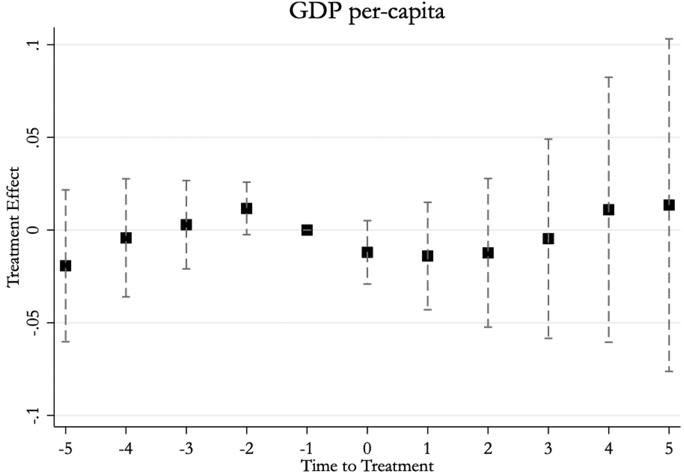
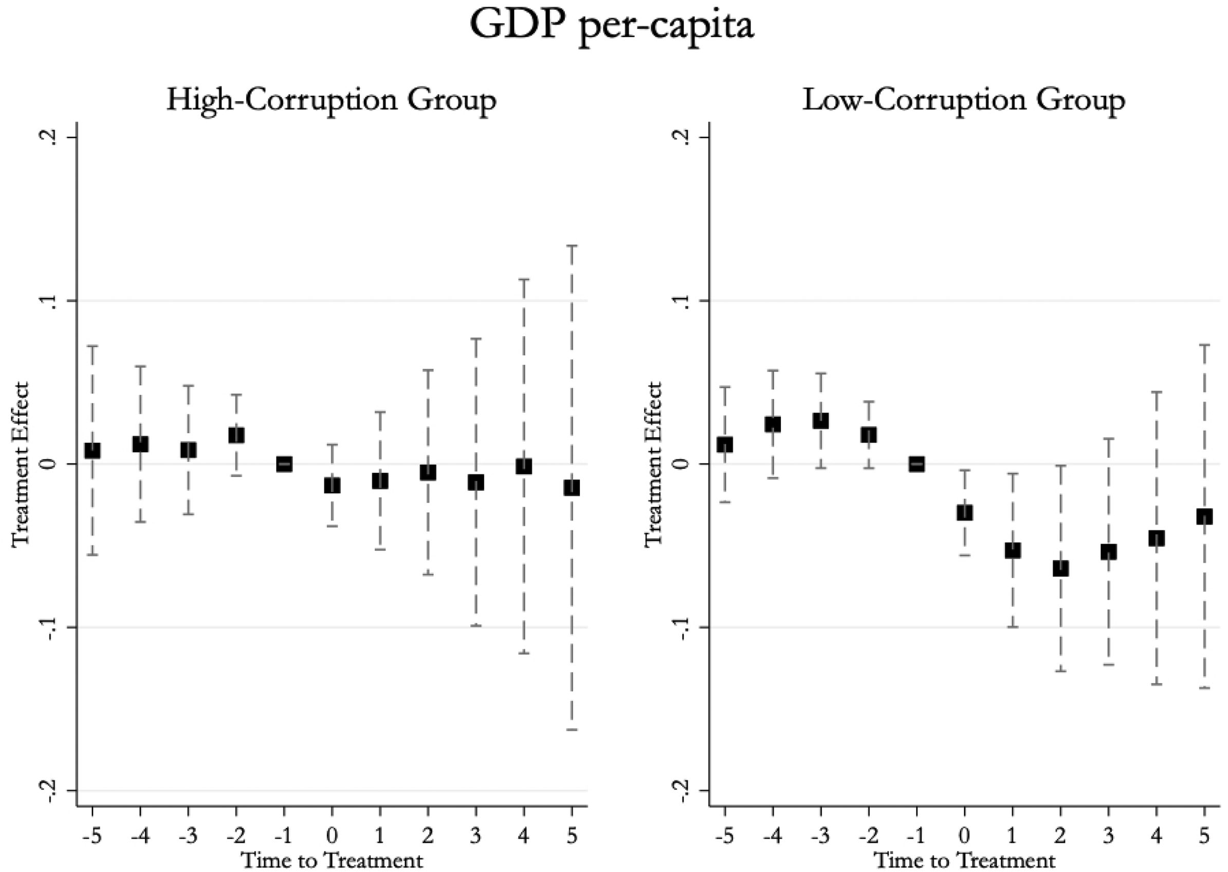
Dynamic effect of FCPA enforcement on GDP per-capita for the high-corruption group (50th percentile or below) and low-corruption group (greater than the 50th percentile).

Table 3.

Dynamic Effect of Corruption Enforcement on GDP Per-Capita for the Full Sample.

	Lower bound (LB)	Coefficient	Upper bound (UB)	Obs.
Year −3	−0.021	0.003	0.027	2,604
Year −2	−0.002	0.012	0.026	2,713
Year 0	−0.029	−0.012	0.005	2,639
Year 1	−0.043	−0.014	0.015	2,460
Year 2	−0.052	−0.012	0.028	2,282

Notes: Lower bound (LB) and upper bound (UB) estimates made with 95% confidence intervals. Bold numbers and double asterisks on the coefficients (**) indicate statistical significance at this level. All estimations include a country-specific time trend. FCPA case data comes from the FCPA Clearinghouse at Stanford Law School. GDP per-capita data comes from PWT Version 9.1.

Table 4.

Dynamic Effect of Corruption Enforcement on GDP Per-Capita for High-Corruption Versus Low-Corruption Groups.

	High-corruption			Low-corruption			Difference?
Year		0–50			50–100
	LB	Coefficient	UB	LL	Coefficient	UB	T-Stat
Year −3	−0.031	0.009	0.048	−0.002	0.027	0.055	−0.720
Year −2	−0.007	0.018	0.042	−0.003	0.018	0.038	−0.012
Year 0	−0.038	−0.013	0.012	−0.056	−0.030**	−0.004	0.910
Year 1	−0.052	−0.010	0.032	−0.100	−0.053**	−0.006	1.322
Year 2	−0.068	−0.005	0.057	−0.127	−0.064**	−0.001	1.300

As shown in Table 3 and Figure 3, FCPA enforcement does not have a significant effect on GDP per capita for the full sample. There is also no impact on GDP per capita for the high-corruption group. However, GDP per capita falls for the low-corruption group. While these effects are not statistically different from one another, they do suggest that the effect of FCPA enforcement is not homogeneous across country groups making the aggregate results less useful. As such, and given our hypothesis regarding bribe-switching, our remaining results focus only on the high- versus low-corruption groups. Graphs summarizing the results using the full sample of data for each of the remaining outcome variables are available upon request.

To gauge the impact of a single FCPA case, we normalize the treatment effects by dividing the coefficients reported in Table 4 by the average number of cases in a given year. For example, in time point 0 (the initial year of the treatment), low-corruption countries experience 1.58 cases on average. Thus, dividing the coefficient for time point 0 (−0.030) by 1.58 shows that a single case reduces logged GDP per capita by 0.019, or GDP per capita by approximately 1.90 percent. We can then repeat this process for each year, normalizing by the appropriate average case counts. After doing so, we find that GDP per capita falls by approximately 1.90 percent in time point 0, 2.7 percent after 1 year (time point 1), and 2.8 percent after 2 years (time point 2). These effects are all statistically significant. Given that the annual growth rate for per capita GDP across countries hovers around 2 percent on average, these are meaningful effects. Normalized coefficients for all our main estimates are summarized in Table A1.

The results suggest that the 1998 FCPA reform may not be fulfilling the broader mandate of the OECD Anti-Bribery Convention of lowering corruption worldwide. In fact, as a more direct indication of this, corruption scores for either the high- or low-corruption groups have not improved. We explore the effect of FCPA enforcement on corruption perceptions using the World Bank Control of Corruption measure and the Political Risk Services Corruption Index. For both measures, a higher value implies less corruption. These results are reported in Table 5, with the 5-year window estimates summarized in Figure 5. There is no evidence that corruption scores improved for either group—on the contrary, corruption perceptions may have worsened in the low-corruption group.¹⁹

Figure 5.

Dynamic effect of FCPA enforcement on corruption perceptions for the high-corruption group (50th percentile or below) and low-corruption group (greater than the 50th percentile).

Table 5.

Dynamic Effect of Corruption Enforcement on Corruption Perceptions Estimator for the High-Corruption Versus Low-Corruption Groups.

	High-corruption			Low-corruption
Year	0–50			50–100			Difference?
World Bank Corruption
	LB	Coefficient	UB	LB	Coefficient	UB	T-Stat
Time Point −3	−0.022	0.013	0.048	−0.014	0.047	0.108	−0.964
Time Point −2	−0.027	−0.002	0.022	−0.020	0.022	0.063	−0.985
Time Point 0	−0.052	−0.017	0.019	−0.069	−0.033	0.003	0.633
Time Point 1	−0.026	0.023	0.073	−0.138	−0.068	0.001	2.115**
Time Point 2	−0.025	0.042	0.108	−0.210	−0.115**	−0.020	2.653**
Political Risk Services Corruption
	LB	Coefficient	UB	LB	Coefficient	UB	T-Stat
Time Point −3	−0.183	−0.032	0.120	−0.292	−0.165	−0.038	1.320
Time Point −2	−0.103	−0.029	0.045	−0.196	−0.101	−0.005	1.161
Time Point 0	−0.139	−0.042	0.055	0.008	0.087**	0.166	−2.014**
Time Point 1	−0.161	0.009	0.179	−0.027	0.126	0.279	−1.002
Time Point 2	−0.231	−0.021	0.190	−0.039	0.196	0.431	−1.347

Notes: Lower bound (LB) and upper bound (UB) estimates made with 95% confidence intervals. Bold numbers and double asterisks on the coefficients/T-statistics (**) indicate statistical significance at this level. For the World Bank Corruption measure, there are an average of 1,065 and 1,139 observations per estimated treatment effect for the high-corruption group and low-corruption group, respectively. Likewise, for PRS, there are an average of 720 and 750 observations per estimated treatment effect for the high-corruption group and low-corruption group, respectively. All estimations include a country-specific time trend. FCPA case data comes from the FCPA Clearinghouse at Stanford Law School. Corruption data comes from WB WGI and the ICRG.

Thus far, the results suggest that the 1998 FCPA reform may not be improving corruption nor total economic activity of the relatively more corrupt countries but may have deleterious effects on the relatively less corrupt, i.e., increasing corruption perceptions and lowering their GDP per capita. To probe deeper into such patterns, we estimate the effect of FCPA enforcement on the expenditure components of GDP per capita. Since expenditure-based GDP is, by identity, the sum of these components, the overall effect of FCPA enforcement on GDP should be consistent with the effect on each component.²⁰ Thus, for instance, if GDP is unchanged, then a fall in any of its components should be accompanied by an increase in any of its remaining components, or a decrease in the case of imports.

The results for the 2-year window are presented in Table 6. To preserve space, results for the full 5-year window are available upon request. FCPA enforcement appears to decrease investment, exports, and imports for both groups. However, the point estimates are larger (in magnitude) for the high-corruption group. The decrease in their investment and exports is accompanied by a large decrease in their imports—recall that the GDP per capita of these countries are unchanged by FCPA enforcement (Table 4). In addition, while insignificant, the effect on government spending is positive in these countries. In contrast, that GDP per capita falls for the low-corruption group is consistent with the point estimates being negative for every component of their GDP.

Table 6.

Dynamic Effect of Corruption Enforcement on GDP Components for the High-Corruption Versus Low-Corruption Groups.

	High-corruption			Low-corruption			Difference?
Year	0–50			50–100
Consumption
	LB	Coefficient	UB	LB	Coefficient	UB	T-Stat
Time Point −3	−0.029	0.009	0.048	−0.040	0.001	0.042	0.286
Time Point −2	−0.037	0.007	0.051	−0.052	−0.015	0.023	0.733
Time Point 0	−0.064	−0.029	0.005	−0.065	−0.022	0.021	−0.242
Time Point 1	−0.072	−0.031	0.010	−0.050	−0.018	0.014	−0.476
Time Point 2	−0.127	−0.061	0.004	−0.075	−0.030	0.014	−0.768
Investment
	LB	Coefficient	UB	LB	Coefficient	UB	T-Stat
Time Point −3	−0.048	0.053	0.153	−0.092	0.000	0.091	0.770
Time Point −2	−0.016	0.040	0.097	−0.065	0.009	0.083	0.661
Time Point 0	−0.140	−0.090**	−0.039	−0.113	−0.057**	−0.002	−0.841
Time Point 1	−0.222	−0.137**	−0.053	−0.128	−0.061	0.007	−1.390
Time Point 2	−0.216	−0.106	0.005	−0.126	−0.043	0.041	−0.891
Government Spending
	LB	Coefficient	UB	LB	Coefficient	UB	T-Stat
Time Point −3	−0.056	0.012	0.081	−0.088	−0.026	0.037	0.800
Time Point −2	−0.012	0.025	0.061	−0.062	0.003	0.067	0.576
Time Point 0	−0.063	0.009	0.081	−0.086	−0.039	0.008	1.105
Time Point 1	−0.087	0.005	0.096	−0.113	−0.052	0.009	1.013
Time Point 2	−0.110	0.022	0.155	−0.158	−0.070	0.018	1.132
Exports
	LB	Coefficient	UB	LB	Coefficient	UB	T-Stat
Time Point −3	0.004	0.078	0.152	−0.203	−0.037	0.129	1.232
Time Point −2	−0.024	0.062	0.149	−0.226	−0.061	0.103	1.305
Time Point 0	−0.161	−0.091	−0.021	−0.110	−0.056**	−0.003	−0.772
Time Point 1	−0.200	−0.093	0.015	−0.173	−0.088**	−0.004	−0.061
Time Point 2	−0.325	−0.180	−0.035	−0.186	−0.089	0.007	−1.019
Imports
	LB	Coefficient	UB	LB	Coefficient	UB	T-Stat
Time Point −3	−0.050	0.018	0.087	−0.129	−0.032	0.064	0.842
Time Point −2	−0.046	0.020	0.085	−0.131	−0.041	0.050	1.056
Time Point 0	−0.130	−0.084**	−0.037	−0.080	−0.037**	0.006	−1.460
Time Point 1	−0.205	−0.133**	−0.061	−0.134	−0.074**	−0.015	−1.230
Time Point 2	−0.288	−0.192**	−0.095	−0.156	−0.085**	−0.015	−1.733

The results suggest that the FCPA may be discouraging investment by preventing corrupt public officials from receiving rents. What is more interesting, however, is that there seems to be some recouping of losses amongst the high-corruption group. That is, rents (corruption perceptions) do not seem to decrease, while the decrease in investment and exports is accompanied by a large decrease in imports, such that total economic activity (GDP per capita) remains unchanged. In contrast, it appears that low-corruption countries are less able to recoup losses—their GDP and all of the components fall after FCPA enforcement.

While there could be other mechanisms by which lost rents and economic activity are recouped after anti-corruption efforts, we put forth a particular hypothesis. If anti-corruption becomes more focused on legal markets, might not this encourage more rent-seeking in illegal markets? Could it thus be that FCPA enforcement induces corrupt public officials to recover lost bribe rents from (legal) investment contracts by extracting more bribes from illegal producers in exchange for allowing more illegal activity? In fact, might the decrease in imports that appear to offset the fall in investments in the high-corruption group be due to an increase in the underreporting of imports? That such anomaly is associated with trade-misinvoicing and, thus, illegal economic activity is indeed suggestive of our hypothesis of bribe-switching between legal and illegal markets. We test this hypothesis in the next section.

Results on Illegal Markets

To test this bribe-switching hypothesis, we compare the effect of FCPA enforcement on the illegal markets of countries whose public officials are more likely, with those whose public officials are less likely, to be already extracting bribes from both legal and illegal markets. To do so, we first group the countries in the same manner as in Section “Empirical Strategy”—according to initial corruption levels. However, a more direct way of ascertaining whether public officials are likely to extract bribes from illegal producers may be to group the countries according to the initial size of their shadow economy (as percentage of GDP), which is a measure of underground transactions. Since relatively more rents can be extracted from a large, rather than a small, shadow economy, one would expect that public officials are more likely to engage in bribe-taking in a large, rather than a small, shadow economy.²¹ Thus, they would be more able to increase bribe-extraction from illegal producers when legal sources of rents dry out.

Our main measure for the size of illegal markets is the size of the shadow economy as percentage of GDP, as constructed by Medina and Schneider (2019). We expect that the shadow economies of countries with initially larger shadow economies increase more than those with initially smaller shadow economies. While the shadow economy measure of Medina and Schneider (2019) is constructed to focus on underground transactions, such transactions may involve both legal and illegal (i.e., prohibited) goods and services. We therefore also use other proxies for illegal activities, although data for these are limited. One proxy is homicide rates, as homicides and other crimes increase with a rise in drug trafficking and other illegal enterprise. Another is tree loss (as a percentage of total hectares), which can capture illegal logging. Finally, we have even sparser data on trade-misinvoicing—a measure that includes the under-reporting of imports to avoid customs duties.²²

The Shadow Economy

Table 7 and Figure 6 suggest that FCPA enforcement increases the shadow economy of countries, irrespective of initial corruption levels. However, consistent with our bribe-switching hypothesis, the point estimates are generally larger for the high-corruption group. The exception is time point 2 (i.e., 2 years after the initial treatment year), where the point estimate for the low-corruption group is higher. However, years 3 through 5 following the initial treatment see significant increases in the size of the shadow economy for the high-corruption group whereas the trend levels out and even starts falling in the low-corruption group (see Figure 6).

Figure 6.

Dynamic effect of FCPA enforcement on shadow economy size for the high-corruption group (50th percentile or below) and low-corruption group (greater than the 50th percentile).

Table 7.

Dynamic Effect of Corruption Enforcement on the Size of the Shadow Economy for the High-Corruption Versus Low-Corruption Groups.

	High-corruption			Low-corruption			Difference?
Year		0–50			50–100
	LB	Coefficient	UB	LL	Coefficient	UB	T-Stat
Time Point −3	−0.921	−0.387	0.147	−0.336	0.013	0.363	−1.229
Time Point −2	−0.813	−0.363	0.087	−0.213	0.027	0.266	−1.498
Time Point 0	0.082	0.494**	0.906	0.033	0.285**	0.537	0.847
Time Point 1	0.010	0.557**	1.105	−0.066	0.342	0.749	0.619
Time Point 2	−0.351	0.371	1.093	0.075	0.642**	1.208	−0.579

After normalization of estimated coefficients, the results show that one FPCA case induces a nearly 0.27 pp increase in the shadow economy of the high-corruption group in time point 0 and a 0.23 pp increase in time point 1. In contrast, the shadow economies of low-corruption countries increase by 0.18 pp in time point 0 and 0.17 pp in time point 1.²³

How large are these magnitudes relative to the bribe rents? A 0.27 pp increase is roughly equivalent to an average of $540 million of additional transactions in the underground economy of the average country in the high-corruption group.²⁴ The average amount of bribe payments in FCPA cases involving countries in this group is $4.3 million, which is almost 1 percent of the growth in the shadow economy. In contrast, a 0.18 pp increase in the shadow economy of the low-corruption group is equivalent to $865 million (0.0018 of $481 billion average GDP in this sample), while the average bribe payments in FCPA cases involving these countries is $3.5 million. Thus, the bribe payments constitute only 0.4 percent of the growth in the shadow economy of this group. Such patterns are consistent with our bribe switching hypothesis, as the extent of rent-seeking from illegal markets should be larger in the high-corruption group.

A similar pattern emerges when we subset the sample according to the initial size of the shadow economy. Table 8 (top panel) and Figure 7 split the sample evenly—with countries in the 50th percentile and above (large-shadow economy group) having an initial (pre-1998) shadow economy that is at least 34 percent of its GDP. The point estimates for the large-shadow group are higher in time point 0 and 1, but again lower in time point 2. However, only the estimate for time point 0 (the year with the first instance of FCPA enforcement) for the large-shadow group is statistically significant—one FCPA case induces a 0.15 pp increase in their shadow economy (Table A3).

Figure 7.

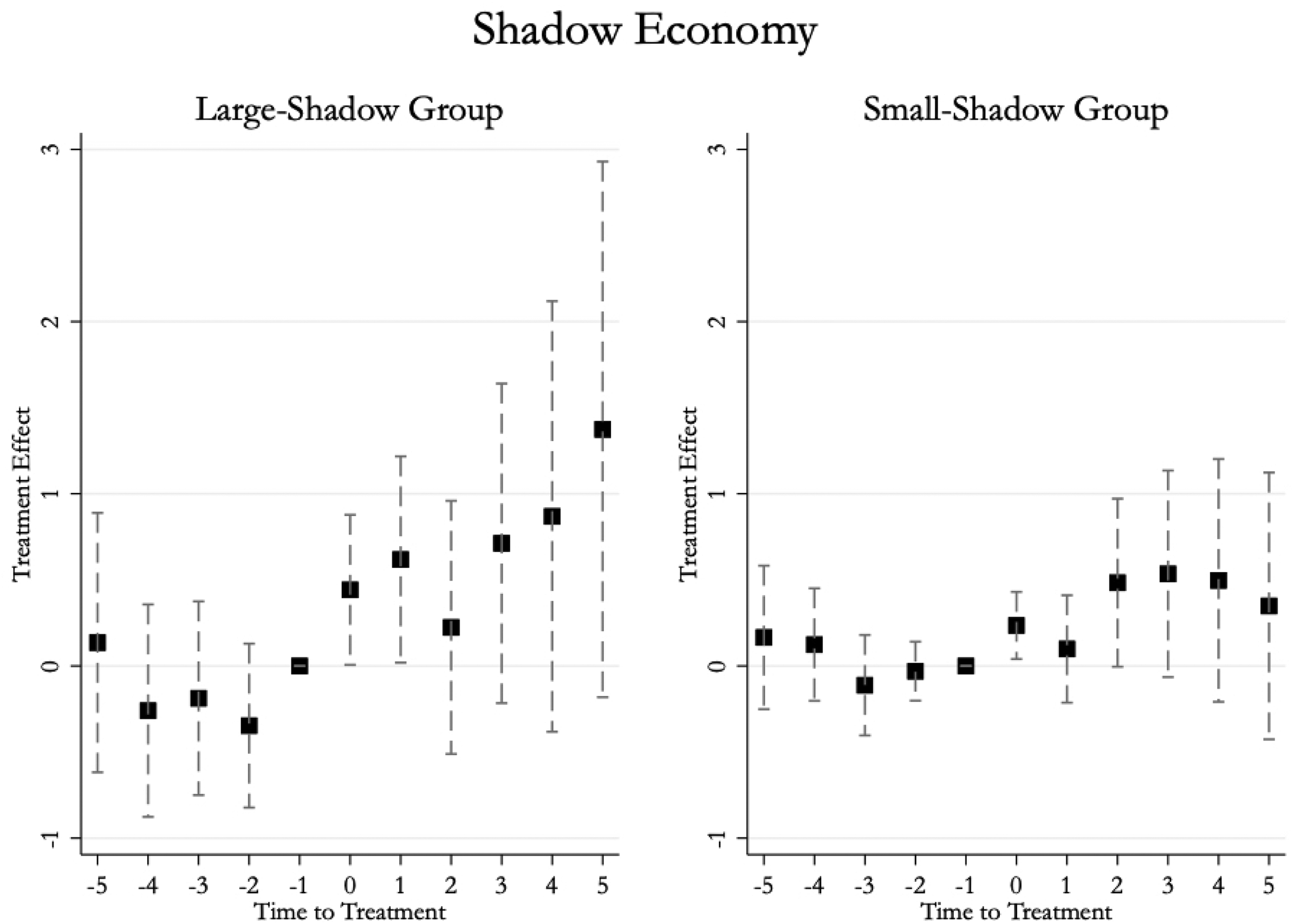
Dynamic effect of FCPA enforcement on shadow economy size for the large-shadow group (50th percentile or above) and small-shadow group (less than the 50th percentile).

Table 8.

Dynamic Effect of Corruption Enforcement on the Size of the Shadow Economy for the High-Corruption Versus Low-Corruption Groups.

	High-corruption			Low-corruption			Difference?
Percentiles		0–50			50–100
	LB	Coefficient	UB	LL	Coefficient	UB	T-Stat
Time Point −3	−0.921	−0.387	0.147	−0.336	0.013	0.363	−1.229
Time Point −2	−0.813	−0.363	0.087	−0.213	0.027	0.266	−1.498
Time Point 0	0.082	0.494**	0.906	0.033	0.285**	0.537	0.847
Time Point 1	0.010	0.557**	1.105	−0.066	0.342	0.749	0.619
Time Point 2	−0.351	0.371	1.093	0.075	0.642**	1.208	−0.579

Notes: Lower bound and upper bound estimates made with 95% confidence intervals. Bold numbers and double asterisks on the coefficients (**) indicate statistical significance at this level. T-statistics assume infinite degrees of freedom and are calculated using a one-tailed test ( ${\hat{α}}_{d}^{H} - {\hat{α}}_{d}^{L}$ ). There are an average of 900 and 897 observations per estimated treatment effect for the high-corruption group and low-corruption group, respectively. All estimations include a country-specific time trend. FCPA case data comes from the FCPA Clearinghouse at Stanford Law School. Shadow economy data comes from Medina and Schneider (2019). Corruption data comes from the WB WGI.

That the point estimates in time point 2 are higher for the small-shadow economy group appears puzzling, as it seems to suggest that there could be more bribe-switching in countries where it is relatively harder to extract bribes from the shadow economy to begin with. Note, however, that because of the 50–50 split of the sample, the small-shadow economy group has many countries with a shadow economy that is between 24 and 34 percent of their GDP—an arguably large percentage. (See Figure B1 in Appendix B.) In fact, the small-shadow economy group includes countries such as Argentina (25.65%), Poland (28.6%), and Romania (31.23%). A likely reason for this is that the composition of the shadow economy can vary across countries—in some the measure might more intensely capture transactions involving prohibited goods and services, while in others it might consist largely of unreported incomes from legal goods and services.

Thus, as an alternative, we also split the sample by grouping countries into the top 75th and bottom 25th percentile of initial shadow economy sizes, where the 75th percentile is 24 percent of GDP. Thus, only countries whose shadow economies are below 24 percent of GDP are included in the small-shadow economy group.²⁵ Table 8 (bottom panel) and Figure 8 now show that the point estimates for all post-treatment years are larger for the large-shadow group.

Figure 8.

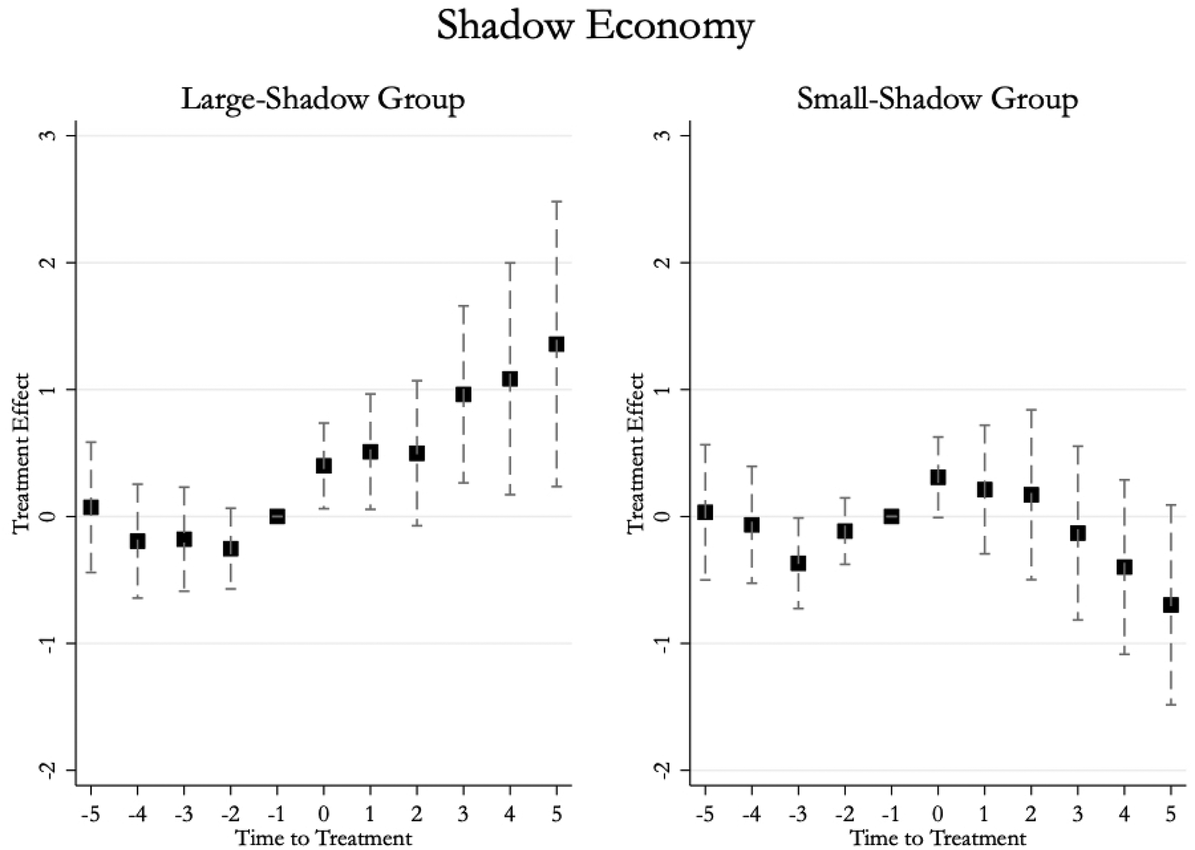
Dynamic effect of FCPA enforcement on shadow economy size for the large shadow group (25th percentile or above) and small-shadow group (less than the 25th percentile).

Other Proxies for Illegal Activities

We consider other proxies for illegal activities. The disadvantage, however, is that we lose many observations, as the data on these proxies are limited. For brevity, we consider the effects of FCPA enforcement using our 50–50 sample splits only. Results using the 25–75 shadow-economy split are available upon request.²⁶ We also only summarize point estimates for the 2-year window; 5-year figure summaries are available upon request. The top and middle panels of Tables 9 and 10 report treatment effects on homicide rates and tree loss. Consistent with our hypothesis, the point estimates, although imprecisely estimated, are generally larger for the large-shadow economy group.

Table 9.

Dynamic Effect of Corruption Enforcement on Other Illegal Activity for the High-Corruption Versus Low-Corruption Groups.

	High-corruption			Low-corruption			Difference?
Year	0–50			50–100
Homicide Rates
	LB	Coefficient	UB	LB	Coefficient	UB	T-Stat
Time Point −3	−0.084	−0.023	0.038	−0.040	0.013	0.066	−0.881
Time Point −2	−0.041	0.008	0.057	−0.053	−0.009	0.034	0.502
Time Point 0	−0.041	0.016	0.073	−0.051	−0.012	0.027	0.807
Time Point 1	−0.028	0.028	0.083	−0.084	−0.024	0.037	1.223
Time Point 2	−0.090	0.002	0.094	−0.113	−0.024	0.066	0.393
Tree Loss
	LB	Coefficient	UB	LB	Coefficient	UB	T-Stat
Time Point −3	−0.020	0.011	0.043	−0.011	0.016	0.043	−0.213
Time Point −2	−0.009	0.013	0.034	−0.010	0.017	0.044	−0.252
Time Point 0	0.002	0.049**	0.096	−0.017	0.038	0.094	0.286
Time Point 1	0.005	0.048**	0.091	−0.022	0.013	0.048	1.231
Time Point 2	0.003	0.062**	0.121	−0.030	0.006	0.042	1.590
Trade Misinvoicing
	LB	Coefficient	UB	LB	Coefficient	UB	T-Stat
Time Point −3	−3.644	−0.535	2.574	−3.463	0.074	3.610	−0.253
Time Point −2	−2.227	−0.489	1.250	−5.059	−2.140	0.779	0.953
Time Point 0	−2.783	−0.258	2.266	−9.425	−1.564	6.296	0.310
Time Point 1	−3.677	0.054	3.784	−7.547	−1.298	4.951	0.364
Time Point 2	−3.006	1.728	6.461	−6.781	0.364	7.510	0.312

Notes: Lower bound and upper bound estimates made with 95% confidence intervals. Bold numbers and double asterisks on the coefficients (**) indicate statistical significance at this level. T-statistics assume infinite degrees of freedom and are calculated using a one-tailed test ( ${\hat{α}}_{d}^{H} - {\hat{α}}_{d}^{L}$ ). For homicide rates, there are an average of 567 and 936 observations per estimated treatment effect for the high-corruption group and low-corruption group, respectively. Likewise, there are an average of 226 and 113 observations for trade misinvoicing and 742 and 420 observations for the tree loss. All estimations include a country-specific time trend. FCPA case data comes from the FCPA Clearinghouse at Stanford Law School. Homicide rates come from the United Nations Office on Drugs and Crime (UNODC). Tree loss data comes from the Global Forest Watch—World Resources Institute. Trade misinvoicing comes from Global Financial Integrity.

Table 10.

Dynamic Effect of Corruption Enforcement on Other Illegal Activity—C&D (2023) for the Large-Shadow (50th Percentile or Above) Versus Small-Shadow Groups (Less than the 50th Percentile).

	Large-shadow group			Small-shadow group			Difference?
Year	50–100			0–50
Homicide Rates
	LB	Coefficient	UB	LB	Coefficient	UB	T-Stat
Time Point −3	−0.111	−0.033	0.044	−0.041	0.002	0.045	−0.776
Time Point −2	−0.066	0.000	0.065	−0.027	0.011	0.049	−0.288
Time Point 0	−0.046	0.017	0.081	−0.046	−0.006	0.034	0.604
Time Point 1	−0.026	0.043	0.113	−0.079	−0.023	0.033	1.463
Time Point 2	−0.094	0.009	0.111	−0.111	−0.030	0.050	0.589
Tree Loss
	LB	Coefficient	UB	LB	Coefficient	UB	T-Stat
Time Point −3	−0.023	0.010	0.043	−0.001	0.023	0.048	−0.643
Time Point −2	−0.011	0.015	0.041	−0.006	0.018	0.042	−0.148
Time Point 0	0.003	0.057**	0.111	−0.016	0.032	0.079	0.688
Time Point 1	0.006	0.052**	0.098	−0.007	0.029	0.066	0.756
Time Point 2	0.003	0.066**	0.129	−0.013	0.032	0.076	0.864
Trade Misinvoicing
	LB	Coefficient	UB	LB	Coefficient	UB	T-Stat
Time Point −3	−3.409	−0.695	2.018	−2.427	1.289	5.005	−0.845
Time Point −2	−2.216	−0.808	0.600	−2.085	−0.201	1.683	−0.506
Time Point 0	−2.422	0.276	2.974	−3.312	−0.607	2.098	0.453
Time Point 1	−3.398	0.536	4.470	−4.613	−0.627	3.358	0.407
Time Point 2	−2.478	2.311	7.100	−5.784	−0.057	5.670	0.622

Notes: Lower bound and upper bound estimates made with 95% confidence intervals. Bold numbers and double asterisks on the coefficients (**) indicate statistical significance at this level. T-statistics assume infinite degrees of freedom and are calculated using a one-tailed test ( ${\hat{α}}_{d}^{H} - {\hat{α}}_{d}^{L}$ ). For homicide rates, there are an average of 560 and 690 observations per estimated treatment effect for the large-shadow group and small-shadow group, respectively. Likewise, there are an average of 253 and 86 observations for trade misinvoicing and 623 and 427 observations for the tree loss, respectively. All estimations include a country-specific time trend. FCPA case data comes from the FCPA Clearinghouse at Stanford Law School. Homicide rates come from the United Nations Office on Drugs and Crime (UNODC). Tree loss data comes from the Global Forest Watch—World Resources Institute. Trade misinvoicing comes from Global Financial Integrity.

Tree loss in particular seems to increase significantly in high-corruption countries. One FCPA enforcement case increases tree loss (as a percentage of hectares) by 0.027 pp in time point 0, 0.019 pp after 1 year, and 0.020 pp after 2 years. Given that the average loss in any given year is only 0.181 pp, these are substantial effects. Further, as will be discussed in the following section, despite the limited data these estimates are remarkably consistent across the five different estimators employed in the paper.

Trade misinvoicing is our most limited measure in terms of data availability. Still, we find that it generally increases for the high-corruption or large-shadow group and decreases for the low-corruption or small-shadow group. While imprecisely estimated, these results are nevertheless supportive of our bribe-switching hypothesis. Recall that FCPA enforcement decreases imports, more so for countries with initially higher levels of corruption. The results on trade misinvoicing suggest that this might be indicative of an increase in the under-reporting of imports.

Conclusion

The US FCPA is a major piece of legislation that enforces against US and non-US entities that are involved in paying bribes to foreign public officials. Its revised version—the post-1998 reform—embodies a commitment to the 1997 OECD Anti-Bribery Convention that establishes anti-bribery as a binding legal principle in the international sphere. This reform also expanded the jurisdictional reach of the FCPA onto foreign countries—with a case count that blossomed from 42 cases focused only on US persons and firms over its first 20 years (1977–1998) to 544 following the 1998 reform. We are the first to estimate the effect of FCPA enforcement post-1998 on the foreign country's economy overall, and its shadow or illegal economy specifically.

We find an adverse, unintended consequence of the FCPA. Foreign countries whose public officials have been involved in bribe-taking from firms and entities subject to the FCPA experience a growth in illegal markets. This is particularly the case in countries that had high levels of corruption to begin with. We also find no benefit to the foreign country's overall level of economic activity or corruption levels. We posit that the FCPA, by decreasing bribe-taking opportunities from the legal sector, e.g., investment contracts, induces corrupt public officials to switch their bribe-taking to illegal markets in order to recover lost rents. In exchange for these bribes, officials enforce less against illegal producers, enabling the growth of illegal activities. We find that one FCPA case alone increases the foreign country's shadow economy by as much as 0.27 pp, its tree loss by 0.027 pp, and its trade misinvoicing by 0.5 pp.

The results suggest that for anti-corruption efforts to be effective, they need to be enforced across all possible transactions—in legal and illegal markets. In highly corrupt countries, or in countries with already large informal markets, it is relatively easy for corruption to move from legal to illegal markets. Outlawing corruption in the legal sector, then, may only encourage corruption to delve further underground and potentially result in more damaging long-run growth prospects. While FCPA enforcers may be considered to be “policeman for the world,” it seems that a more comprehensive anti-corruption program may be necessary to reduce corruption overall.

Supplemental Material

sj-docx-1-pfr-10.1177_10911421241248719 - Supplemental material for Bribe-Switching

Supplemental material, sj-docx-1-pfr-10.1177_10911421241248719 for Bribe-Switching by Jamie Bologna Pavlik and Desiree Desierto in Public Finance Review

Footnotes

Declaration of Conflicting Interests

The authors declared no potential conflicts of interest with respect to the research, authorship, and/or publication of this article.

Funding

The authors received no financial support for the research, authorship, and/or publication of this article.

ORCID iD

Jamie Bologna Pavlik

Supplemental Material

Supplemental material for this article is available online.

Notes

Author Biographies

Jamie Bologna Pavlik is associate professor of Agricultural and Applied Economics at Texas Tech University. She conducts research in economic growth and development, with particular emphasis on the role of institutions and the problem of corruption.

Desiree Desierto is assistant professor at the Economics Department of George Mason University. She conducts research in political economy and economic history.

Appendices

References

Arbatskaya

Mialon

H. M.

. 2020. “The Impact of the Foreign Corrupt Practices Act on Competitiveness, Bribery, and Investment.” American Law and Economics Review 22 (1): 105–126. https://doi.org/10.1093/aler/ahaa004.

Athey

Imbens

G. W.

. 2018. “Design-Based Analysis in Difference-In-Differences Settings with Staggered Adoption.” NBER Working Papers 24963, National Bureau of Economic Research, Inc.

Becker

G. S.

Murphy

K. M.

Grossman

. 2006. “The Market for Illegal Goods: The Case of Drugs.” Journal of Political Economy 114 (1): 38–60. https://doi.org/10.1086/498918.

Bologna

Ross

. 2015. “Corruption and Entrepreneurship: Evidence from Brazilian Municipalities.” Public Choice 165 (1): 59–77. https://doi.org/10.1007/s11127-015-0292-5.

Borlea

S. N.

Achim

M. V.

Miron

M. G. A.

. 2017. “Corruption, Shadow Economy and Economic Growth: An Empirical Survey Across the European Union Countries.” Studia Universitatis “Vasile Goldis” Arad—Economics Series 27 (2): 19–32. https://doi.org/10.1515/sues-2017-0006.

Borusyak

Jaravel

. 2017. “Revisiting Event Study Designs.” Working Paper.

Brewster

2017. “Enforcing the FCPA: International Resonance and Domestic Strategy.” Virginia Law Review 103: 1611. https://scholarship.law.duke.edu/faculty_scholarship/3779.

Burgess

Hansen

Olken

B. A.

Potapov

Sieber

. 2012. “The Political Economy of Deforestation in the Tropics.” The Quarterly Journal of Economics 127 (4): 1707–1754. https://doi.org/10.1093/qje/qjs034.

Callaway

Sant’Anna

P. H.

. 2021. “Difference-in-Differences With Multiple Time Periods.” Journal of Econometrics 225 (2): 200–230. https://doi.org/10.1016/j.jeconom.2020.12.001.

10.

Campos

Engel

Fischer

R. D.

Galetovic

. 2021. “The Ways of Corruption in Infrastructure: Lessons from the Odebrecht Case.” Journal of Economic Perspectives 35 (2): 171–190. https://doi.org/10.1257/jep.35.2.171.

11.

Cassin

R. L.

2018. “Petrobras Reaches $1.78 Billion FCPA Resolution.” The FCPA Blog.

12.

Cassin

2020. “Goldman Sachs Reaches $3.3 Billion Resolution of Malaysia FCPA Violations.” The FCPA Blog.

13.

Cengiz

Dube

Lindner

Zipperer

. 2019. “The Effect of Minimum Wages on Low-Wage Jobs.” The Quarterly Journal of Economics 134 (3): 1405–1454. https://doi.org/10.1093/qje/qjz014.

14.

Choi

J. P.

Thum

. 2005. “Corruption and the Shadow Economy.” International Economic Review 46 (3): 817–836. https://doi.org/10.1111/j.1468-2354.2005.00347.x.

15.

Christensen

H. B.

Maffett

M. G.

Rauter

. 2022. “Policeman for the World: The Impact of Extraterritorial FCPA Enforcement on Foreign Investment and Internal Controls.” The Accounting Review 97 (5): 189–219. https://doi.org/10.2308/TAR-2020-0564.

16.

Cieślik

Goczek

. 2018. “Control of Corruption, International Investment, and Economic Growth–Evidence From Panel Data.” World Development 103: 323–335. https://doi.org/10.1016/j.worlddev.2017.10.028.

17.

Colonnelli

Prem

. 2022. “Corruption and Firms.” Review of Economic Studies 89 (2): 695–732. https://doi.org/10.1093/restud/rdab040.

18.

de Chaisemartin

D’Haultfoeuille

. 2022. “Two-Way Fixed Effects and Differences-in-Differences with Heterogeneous Treatment Effects: A Survey.” Technical Report, National Bureau of Economic Research.

19.

de Chaisemartin

D’Haultfœuille

. 2020. “Two-Way Fixed Effects Estimators With Heterogeneous Treatment Effects.” American Economic Review 110 (9): 2964–2996. https://doi.org/10.1257/aer.20181169.

20.

de Chaisemartin

D’Haultfœuille

. 2023. “Difference-in-Differences Estimators of Intertemporal Treatment Effects.” NBER Working Paper No. 29873.

21.

Desierto

D. A.

2021. “Grand Corruption by Theft and Bribery.” Working Paper.

22.

Desierto

D. A.

Nye

J. V. C.

. 2017. “Prohibition Versus Taxation in Corrupt Environments.” Journal of Institutional and Theoretical Economics (JITE) 173 (2): 239–252. https://doi.org/10.1628/093245616X14618208477808.

23.

Donchev

Ujhelyi

. 2014. “What do Corruption Indices Measure?” Economics & Politics 26 (2): 309–331. https://doi.org/10.1111/ecpo.12037.

24.

Dreher

Kotsogiannis

McCorriston

. 2009. “How do Institutions Affect Corruption and the Shadow Economy?” International Tax and Public Finance 16 (6): 773–796. https://doi.org/10.1007/s10797-008-9089-5.

25.

Dreher

Schneider

. 2010. “Corruption and the Shadow Economy: An Empirical Analysis.” Public Choice 144 (1): 215–238. https://doi.org/10.1007/s11127-009-9513-0.

26.

Dreher

Siemers

L.-H.

. 2009. “The Nexus Between Corruption and Capital Account Restrictions.” Public Choice 140 (1): 245–265. https://doi.org/10.1007/s11127-009-9423-1.

27.

Dutta

Sobel

. 2016. “Does Corruption Ever Help Entrepreneurship?” Small Business Economics 47 (1): 179–199. https://doi.org/10.1007/s11187-016-9728-7.

28.

El-Shagi

2005. “A Legal Crime: Capital Controls as an Act of Corruption.” Technical Report, mimeo, University of Mannheim.

29.

Goodman-Bacon

2018. “Difference-in-Differences With Variation in Treatment Timing.” Working Paper 25018, National Bureau of Economic Research.

30.

Graham

Stroup

. 2016. “Does Anti-Bribery Enforcement Deter Foreign Investment?” Applied Economics Letters 23 (1): 63–67. https://doi.org/10.1080/13504851.2015.1049333.

31.

Gründler

Potrafke

. 2019. “Corruption and Economic Growth: New Empirical Evidence.” European Journal of Political Economy 60: 101810. https://doi.org/10.1016/j.ejpoleco.2019.08.001.

32.

Hindriks

Keen

Muthoo

. 1999. “Corruption, Extortion and Evasion.” Journal of Public Economics 74 (3): 395–430. https://doi.org/10.1016/S0047-2727(99)00030-4.

33.

Hines

James R.

1995. “Forbidden Payment: Foreign Bribery and American Business After 1977.” NBER Working Papers 5266, National Bureau of Economic Research, Inc.

34.

Johnson

Kaufmann

Zoido-Lobaton

. 1998. “Regulatory Discretion and the Unofficial Economy.” American Economic Review 88 (2): 387–392. https://www-jstor-org-443.web.bisu.edu.cn/stable/116953.

35.

Lippitt

A. H.

2013. “An Empirical Analysis of the Foreign Corrupt Practices Act.” Virginia Law Review 99 (8): 1893–1930. https://www-jstor-org-443.web.bisu.edu.cn/stable/23611100.

36.

Mauro

1995. “Corruption and Growth.” The Quarterly Journal of Economics 110 (3): 681–712. https://doi.org/10.2307/2946696.

37.

Medina

Schneider

. 2019. “Shedding Light on the Shadow Economy: A Global Database and the Interaction With the Official One.” CESifo Working Paper.

38.

P. H.

2001. “Corruption and Economic Growth.” Journal of Comparative Economics 29 (1): 66–79. https://doi.org/10.1006/jcec.2000.1703.

39.

Olken

B. A.

2007. “Monitoring Corruption: Evidence From Field Experiments in Indonesia.” Journal of Political Economy 115 (2): 417–452. https://doi.org/10.1086/517935

40.

Olken

B. A.

2009. “Corruption Perceptions vs. Corruption Reality.” Journal of Public Economics 93 (7-8): 950–964. https://doi.org/10.1016/j.jpubeco.2009.03.001.

41.

Olken

B. A.

Pande

. 2012. “Corruption in Developing Countries.” Annual Review of Economics 4 (1): 479–509. https://doi.org/10.1146/annurev-economics-080511-110917.

42.

Roth

2024. “Interpreting Event-Studies from Recent Difference-in-Differences Methods.” Working Paper.

43.

Sun

Abraham

. 2018. “Estimating Dynamic Treatment Effects in Event Studies With Heterogeneous Treatment Effects.” Papers 1804.05785, arXiv.org.

44.

Wei

S.-J.

2000. “How Taxing is Corruption on International Investors?” Review of Economics and Statistics 82 (1): 1–11. https://doi.org/10.1162/003465300558533.

45.

Zakharov

2019. “Does Corruption Hinder Investment? Evidence From Russian Regions.” European Journal of Political Economy 56: 39–61. https://doi.org/10.1016/j.ejpoleco.2018.06.005.

Supplementary Material

Please find the following supplemental material available below.

For Open Access articles published under a Creative Commons License, all supplemental material carries the same license as the article it is associated with.

For non-Open Access articles published, all supplemental material carries a non-exclusive license, and permission requests for re-use of supplemental material or any part of supplemental material shall be sent directly to the copyright owner as specified in the copyright notice associated with the article.

0.00 MB

2.35 MB