Cronbach’s Coefficient Alpha

Abstract

This study disproves the following six common misconceptions about coefficient alpha: (a) Alpha was first developed by Cronbach. (b) Alpha equals reliability. (c) A high value of alpha is an indication of internal consistency. (d) Reliability will always be improved by deleting items using “alpha if item deleted.” (e) Alpha should be greater than or equal to .7 (or, alternatively, .8). (f) Alpha is the best choice among all published reliability coefficients. This study discusses the inaccuracy of each of these misconceptions and provides a correct statement. This study recommends that the assumptions of unidimensionality and tau-equivalency be examined before the application of alpha and that structural equation modeling (SEM)–based reliability estimators be substituted for alpha when one of these conditions is not satisfied. This study also provides formulas for SEM-based reliability estimators that do not rely on matrix notation and step-by-step explanations for the computation of SEM-based reliability estimates.

Keywords

reliability coefficient alpha tau-equivalency internal consistency multidimensionality multiple-factor model

Although many methods for estimating the reliability of test scores have been proposed (for a complete review of the estimation methods, see, e.g. Feldt & Brennan, 1989; Haertel, 2006), this study focuses on Cronbach’s (1951) coefficient alpha (hereinafter referred to as “alpha”), which estimates reliability by using data from a single test administration. Alpha, conceived as an “internal consistency” coefficient, is the most frequently used reliability coefficient (which is to be interpreted as an estimator or an estimate of reliability, depending on the context) in organizational research.

Previous studies such as Cortina (1993) and Schmitt (1996) have played an important role in providing a better understanding of alpha for organizational researchers. The influence of their seminal articles is remarkable; Cortina (1993) and Schmitt (1996) appear within the list of the 10 most cited articles among all the papers that were published during the past 20 years in the Journal of Applied Psychology and Psychological Assessment, respectively (Harzing, 2013). While their comprehensive reviews still provide valuable guidance for organizational researchers, there is an increasing need for a review that discusses the latest studies and that offers an updated perspective on the issue.

The influence of Cronbach (1951) has not been overshadowed. His groundbreaking paper has been cited by more than 22,000 studies, which is the largest number of citations for any paper published in Psychometrika (Harzing, 2013). Cronbach (2004) declared it to be “[another sign] of success” that “there were very few later articles by others criticizing parts of my argument” (p. 393). Despite the optimistic assessment provided by Cronbach (2004), criticisms of alpha have been actively published in the past decade.

However, such research does not offer a practical aid to organizational researchers for several reasons. First, the latest theoretical reviews of alpha can only be found in psychometrics journals, such as Psychometrika. As Sijtsma (2009a) noted, psychometricians, who are theorists of measurement, have been distanced from other social scientists, who are practitioners of measurement. Studies in psychometrics are increasingly using advanced mathematics that most social scientists cannot easily understand. Second, previously published papers in psychometrics have typically focused on specific subjects within the field, and these papers are thus less helpful for understanding the broader outline of the field. Therefore, a comprehensive study on the historical background of alpha and the practical issues arising from using it as a reliability coefficient would be particularly helpful to organizational researchers.

The current study seeks to respond to such a research need. In the next section, we develop our analyses on test score reliability by focusing on six common misconceptions about alpha that are frequently held by organizational researchers. For example, one may believe that Cronbach first proposed alpha because it is named “Cronbach’s alpha”; one may also contend that alpha should be regarded as the best available reliability coefficient because so many researchers use it in practice. Disproving such misconceptions will enable organizational researchers to make better decisions on fundamental issues such as what to call, how to use, and even whether to use alpha. After the “misconception” section, we present the formulas and procedures of alternatives to coefficient alpha for reliability estimation when the prerequisite assumptions for alpha are suspected to be violated. In presenting this information, we show that reliability estimators based on structural equation modeling (SEM) may be effectively used for all of the situations in which violation of the assumptions for alpha is suspected.

Before addressing the misconceptions about alpha, however, we first note the true score modeling of the test score $X$ and the definition of test score reliability in classical test theory. Consider a test consisting of $k$ dichotomously or polytomously scored items. The test score $X$ is defined as the sum of $k$ “observed” item scores $X_{i}$ ; $X = \sum_{i = 1}^{k} X_{i}$ . The true score model states that $X$ is composed of two unobserved scores, namely, the true score $T$ and error $e$ : $X = T + e$ . The reliability of test scores is defined as the product-moment correlation ( $ρ_{X X^{'}}$ ) between the scores $X$ and $X^{'}$ ( $= T + e^{'}$ ) from two parallel forms of a test (Lord & Novick, 1968; Novick & Lewis, 1967). In a population, $ρ_{X X^{'}}$ is equal to the squared correlation ( $ρ_{X T}^{2}$ ) between $X$ and $T$ , which is also equal to the ratio of the true score variance ( $σ_{T}^{2}$ ) to the test score variance ( $σ_{X}^{2}$ ). Formally,

ρ_{X X^{'}} = ρ_{X T}^{2} = \frac{σ_{T}^{2}}{σ_{X}^{2}} = \frac{σ_{T}^{2}}{σ_{T}^{2} + σ_{e}^{2}}

Given sample data from a single administration of a test, alpha estimates the reliability of test scores for a population of examinees of interest, as defined in Equation 1.

Common Misconceptions About Alpha

Common Misconception: Alpha Was First Developed by Cronbach

Although subsequent researchers provide more elaborate interpretations, newer proofs, and more meaningful modifications to earlier works, academia recognizes the researcher who originated a formula to the greatest extent. In our field, it is difficult to imagine not using the originator’s name for a formula. Thus, Cronbach is commonly considered to have initially proposed the formula in question.

The Spearman-Brown formula was presented approximately 100 years ago. The formula was so named because it was published independently by Spearman (1910) and Brown (1910) in the same issue of the same journal, the British Journal of Psychology. Let $X_{a}$ and $X_{b}$ denote the first- and second-half test scores, respectively, such that $X = X_{a} + X_{b}$ ; let $σ_{X}^{2}$ , $σ_{a}^{2}$ , and $σ_{b}^{2}$ denote the variances of $X$ , $X_{a}$ , and $X_{b}$ , respectively; and let $σ_{a b}$ and $ρ_{a b}$ denote the covariance and the product-moment correlation, respectively, between $X_{a}$ and $X_{b}$ . The Spearman-Brown formula ( $ρ_{S B}$ ) states that the reliability of the full-length test scores ( $ρ_{X X^{'}}$ ) can be estimated by correcting the correlation between the two half-test scores as follows:

ρ_{S B} = \frac{2 ρ_{a b}}{1 + ρ_{a b}}

The Spearman-Brown formula is based on the assumption that the half tests are parallel and thus that the score variances of the split-halves are equal. General formulas that are applicable when the variances differ were independently proposed by Flanagan (1937), Rulon (1939), and Mosier (1941).

However, these split-half reliability formulas yield different results depending on how the halves are split. To resolve this issue, Kuder and Richardson (1937) proposed a reliability formula (called “KR-20”) that can be used for data on dichotomously scored items (e.g., $X_{i} =$ 0 or 1). When $p_{i}$ is the percentage of correct responses for item $i$ and k is the number of items, the KR-20 formula is expressed as follows:

ρ_{K R - 20} = \frac{k}{k - 1} (1 - \frac{\sum_{i = 1}^{k} p_{i} (1 - p_{i})}{σ_{X}^{2}})

Guttman (1945) believed that the preceding studies set too many assumptions to obtain a reliability coefficient and thus presented six reliability estimators. The only assumption required for Guttman’s estimators was the independence between the error scores of the items (i.e., $σ_{e_{i} e_{j}} = 0$ ). Guttman (1945) referred to the six estimators as lower bounds of the reliability rather than as reliability coefficients. In the following is a list of three of the six lower bounds— $λ_{2}$ , $λ_{3}$ , and $λ_{4}$ ( $λ_{4}$ was proposed as the lower bound of the split-half reliability):

λ_{2} = \frac{\underset{i \neq j}{Σ Σ} σ_{i j} + \sqrt{\frac{k}{k - 1} \underset{i \neq j}{Σ Σ} σ_{i j}^{2}}}{σ_{X}^{2}};

λ_{3} = α = \frac{k}{k - 1} (1 - \frac{\sum_{i = 1}^{k} σ_{i}^{2}}{σ_{X}^{2}}); a n d

λ_{4} = 2 (1 - \frac{σ_{a}^{2} + σ_{b}^{2}}{σ_{X}^{2}})

Cronbach (1951) proposed alpha, as expressed in Equation 5, which enables KR-20 to be applied to polytomously scored item data (e.g., $X_{i} =$ 0, 1, 2, or 3). The Spearman-Brown formula was most frequently used to calculate split-half reliability at that time, but Cronbach (1951) criticized the formula, stating that it increased calculation error when it was used for cases in which the variance differed between the split-halves. Cronbach (1951) used Guttman’s $λ_{4}$ to prove that alpha (i.e., $λ_{3}$ ) is the mean of the $λ_{4}$ values that are computed for all possible split-halves. Guttman’s $λ_{4}$ is algebraically equivalent to the formulas proposed by Flanagan (1937), Rulon (1939), and Mosier (1941).

As we have shown previously, Guttman’s (1945) $λ_{3}$ is equivalent to alpha, but it is not Guttman who first proposed the formula. Hoyt (1941) applied an analysis of variance (ANOVA) model to elicit the reliability coefficient, and its derivation arrived at a formula identical to alpha (Cronbach, 1951). Additionally, the KR-20 formula is another expression of alpha when it is applied to dichotomously scored items (Note $σ_{i}^{2} = p_{i} (1 - p_{i})$ ).

This argument does not suggest that Cronbach intercepted the achievements of previous researchers. Although the coefficient is typically called Cronbach’s alpha, Cronbach never named the coefficient after himself. In fact, Cronbach (2004) shied away from the name Cronbach’s alpha, stating the following: “To make so much use of an easily calculated translation of a well-established formula scarcely justifies the fame it has brought me. It is an embarrassment to me that the formula became conventionally known as ‘Cronbach’s $α$ ’” (p. 397).

It is the users (or, rather, the “consumers”) of the formula who credited Cronbach (1951) rather than Hoyt (1941) or Guttman (1945), both of whom preceded Cronbach in introducing algebraically equivalent formulas. Different positioning strategies of these studies could have led users to perceive the formulas to be different even though they yielded the same results. First, alpha was positioned as a general reliability coefficient. Cronbach (1951) mathematically proved that alpha, the general formula of KR-20, can also be the general formula for split-half reliability formulas. That is, Cronbach’s proof that the formulas that were previously thought to be unrelated are actually connected to each other led alpha to be positioned as a representative and comprehensive formula, not merely one of many reliability coefficients. Such positioning of alpha sharply contrasts with that of $λ_{3}$ , which was merely one of six formulas proposed by Guttman (1945). Second, alpha was positioned as a reliability coefficient. Whereas Guttman (1945) referred to $λ_{3}$ as the lower bound of reliability, Cronbach (1951) presented alpha as a reliability coefficient. Users likely preferred to view alpha as a reliability coefficient than to view alpha as the lower bound of reliability.

Interestingly, alpha was not the best reliability coefficient even at the time of Cronbach’s (1951) publication. To find a better alternative than alpha, it is natural to assume that recent studies on reliability should be cited. Contrary to such expectations, a superior alternative already existed even before the name of alpha was proposed by Cronbach (1951). Guttman (1945) referred to $λ_{1}$ as “a simple lower bound,” $λ_{3}$ (=alpha) as “an intermediate lower bound,” and $λ_{2}$ as “a better lower bound” and proved that $λ_{1} \leq λ_{3} \leq λ_{2} \leq ρ_{X X^{'}}$ . That is, under the condition of independence between item errors, $λ_{2}$ is always superior to or as good as alpha. From the modern perspective, $λ_{3}$ , an inferior alternative, may not have merited publication. Guttman proposed $λ_{3}$ because its formula was simpler and easier to calculate than that of $λ_{2}$ . In the 1940s, calculation with computers was unimaginable, and the ease of calculation was a virtue in a world in which all calculations were performed by hand.

Common Misconception: Alpha Equals Reliability

In the current organizational research literature, alpha is often considered to be the equivalent of the reliability of test scores. However, it is difficult to find explanations as to whether alpha is larger or smaller than reliability when the prerequisites for alpha to be the reliability coefficient are not fulfilled. Therefore, alpha can be easily misconceived to always be equal to reliability or at least to be an unbiased estimator of reliability.

Under the Assumption of Uncorrelated Item Errors

Guttman (1945, p. 274) proposed that $λ_{3}$ (i.e., alpha) could be the reliability coefficient “if and only if the variances and covariances of the expected scores on the items are all equal.” An even more sophisticated proof was proposed by Novick and Lewis (1967), who suggested the concept of the essentially tau-equivalent condition between items. Let us describe the classical true score model, in terms of factor analysis, to explain the proof by Novick and Lewis.

In the classical true score model, the observed score for item $i$ (=1,…, $k$ ) can be decomposed into two or three components as follows:

X_{i} = T_{i} + e_{i} = μ_{i} + λ_{i} T + e_{i},

where $T_{i} = μ_{i} + λ_{i} T$ , $\sum λ_{i} = 1$ , and $\sum μ_{i} = 0$ . The expression $X_{i} = μ_{i} + λ_{i} T + e_{i}$ in Equation 7 is referred to as a single-factor model in psychometric analysis. In the single-factor model, $μ_{i}$ are constants that allow for differences in item-score means and the sum to be zero across the items, and $λ_{i}$ are the factor loadings, which represent the proportionate functional lengths of the items. The similarity between the items may vary depending on which constraints are imposed on $λ_{i}$ and the interitem error covariances. For example, if $μ_{i} = 0$ , $λ_{i} = λ_{j}$ , and $σ_{e_{i}}^{2} = σ_{e_{j}}^{2}$ for all $i$ and $j$ , the items are parallel such that $σ_{X_{i}}^{2} = σ_{X_{j}}^{2}$ and $σ_{X_{i} X_{j}} = σ_{T}^{2} / k^{2}$ . If $λ_{i} = λ_{j}$ for all $i$ and $j$ , the items are essentially tau-equivalent, such that $σ_{X_{i}}^{2} \neq σ_{X_{j}}^{2}$ but $σ_{X_{i} X_{j}} = σ_{T}^{2} / k^{2}$ . The term essentially indicates that an addition of a constant ( $μ_{i}$ ) has essentially no effect on the variances or covariances of the item scores. If no constraints (except the constraints $\sum λ_{i} = 1$ and $\sum μ_{i} = 0$ ) are imposed, the items have congeneric similarity, such that $σ_{X_{i}}^{2} \neq σ_{X_{j}}^{2}$ and $σ_{X_{i} X_{j}}$ may not be equal to each other.

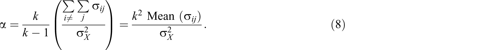
Now consider another expression of alpha that is based on the average of all $k (k - 1)$ observed-score covariances between items:

α = \frac{k}{k - 1} (\frac{\sum_{i \neq} \sum_{j} σ_{i j}}{σ_{X}^{2}}) = \frac{k^{2} M e a n (σ_{i j})}{σ_{X}^{2}}

This expression is simply derived from the fact that $σ_{X}^{2} = \sum_{i} \sum_{j} σ_{i j} = \sum_{i} σ_{i}^{2} + \sum_{i \neq} \sum_{j} σ_{i j}$ , where $σ_{i}^{2} \equiv σ_{X_{i}}^{2}$ and $σ_{i j} \equiv σ_{X_{i} X_{j}}$ . If items are “at least” essentially tau-equivalent (i.e., $σ_{X_{i} X_{j}} = σ_{T}^{2} / k^{2}$ for all $i$ and $j$ ), the numerator in Equation 8 becomes equal to the true score variance $σ_{T}^{2}$ . That is, alpha is equal to $ρ_{X X^{'}}$ when the essentially tau-equivalent condition holds among the items. Elaborating this statistical point, Novick and Lewis (1967) demonstrated that the necessary and sufficient condition for alpha to be reliability is the essential tau-equivalency and that, if this condition is not met, alpha is smaller than reliability.

Alpha has typically been referred to as a reliability coefficient rather than a lower-bound estimate; however, the latter is a more correct description in a strict sense. The concept of lower bound enables us to better understand the characteristics of alpha, which might seem counterintuitive if we considered alpha to be a reliability coefficient.

First, we rethink the meaning of Cronbach’s (1951) mathematical proof. The average of the split-half reliability estimates that are acquired from all possible split-halves is an intuitively attractive concept. However, human intuition is occasionally deceived. One important point is usually overlooked: Guttman’s $λ_{4}$ is not a reliability coefficient; rather, it is a lower bound of reliability. The concept of a lower bound to reliability yields the understanding that Mean ( $λ_{4}$ )—the mean of the $λ_{4}$ values from all possible split-halves—does not produce a maximum value that is close to the actual reliability; however, Max ( $λ_{4}$ )—the maximum of the $λ_{4}$ values—does approximate reliability.

Second, alpha is negative when the average of the interitem score covariances is negative (see Equation 8; Cronbach & Hartmann, 1954). Many textbooks explain that alpha has a value between zero and one. Upon reading this explanation, one may assume that it is impossible for alpha to have a negative value, irrespective of any prerequisite condition. However, in practice, alpha may have a negative value in some situations, for example, where an item is negatively worded but is accidentally not reversely scored in a personality scale (Sijtsma, 2009a) or where an item has a negative discrimination in a multiple-choice achievement test. All reliability coefficients do not have the same problem as alpha; we will show later that SEM estimators of reliability (i.e., Equation 16 and 19) are always non-negative.

Third, alpha may be smaller than one even when no measurement error exists. By definition, the reliability of test scores must be one when no measurement error exists. Thus, one might assume that alpha will also be one when the measurement error variance is zero. To examine this statement, let us take an exemplary case in which homogeneity (i.e., unidimensionality) across items is satisfied but in which the essentially tau-equivalent condition is not satisfied. Consider a three-item test. The following variance-covariance matrix for the three-item scores is one such matrix that meets the homogeneous condition:

Σ = [\begin{matrix} \begin{matrix} 1.0 & 1 .0 & 2.0 \end{matrix} \\ \begin{matrix} 1 .0 & 1.0 & 2.0 \end{matrix} \\ \begin{matrix} 2.0 & 2.0 & 4 .0 \end{matrix} \end{matrix}]

The computation of alpha based on this matrix results in $α = .9375$ , which is less than one (i.e., perfect reliability). This example effectively demonstrates that alpha is a lower bound of reliability when it does not satisfy the condition of being essentially tau-equivalent. This example also suggests the need for the items to be standardized before an aggregate score is computed when items are combined with radically different variances. The value of standardized alpha for this example is one. The value of a congeneric reliability coefficient (which will be described later) for this example is also one.

Without the Assumption of Uncorrelated Item Errors

Thus far, we have assumed that item errors ( $e_{i}$ ) are independent from each other (i.e., $σ_{e_{i} e_{j}} = 0$ ). We now consider the following question: “When the errors are correlated, would alpha increase or decrease, compared to when the errors are independent?” To answer the question, we first note that the variance of the observed item scores ( $σ_{X_{i}}^{2}$ ) is not affected by the non-zero correlation between item errors, but when the errors are not independent, the interitem covariance ( $σ_{X_{i} X_{j}}$ ) changes to $σ_{T}^{2} / k^{2} + σ_{e_{i} e_{j}}$ , not to $σ_{T}^{2} / k^{2}$ . That is, collectively,

\sum_{i \neq} \sum_{j} σ_{X_{i} X_{j}} = (\frac{k - 1}{k}) σ_{T}^{2} + \sum_{i \neq} \sum_{j} σ_{e_{i} e_{j}}

Thus, test score reliability should be expressed as follows:

ρ_{X X^{'}} = \frac{σ_{T}^{2}}{σ_{X}^{2}} = \frac{σ_{T}^{2}}{σ_{T}^{2} + \sum_{i} σ_{e_{i}}^{2} + \sum_{i \neq} \sum_{j} σ_{e_{i} e_{j}}}

Lucke (2005) developed the idea expressed in Equations 9 and 10 into more sophisticated proofs, which generate the following implications. First, correlated item errors affect alpha and classical reliability in the opposite direction. Positively correlated item errors decrease the value of reliability but make alpha overestimate (i.e., inflate) the true reliability.

Second, the impact of correlated item errors on alpha and classical reliability strictly occurs through the sum of interitem error covariances. The internal structure of interitem error covariances (e.g., autocorrelated, moving average) is irrelevant. The similarity between the items (e.g., parallel, tau-equivalent, congeneric) is also irrelevant.

Third, the necessary and sufficient condition for alpha to be equivalent to classical reliability should be that the sum of interitem error covariances equals the deviance from tau-equivalency. If the former is smaller than the latter, alpha underestimates reliability. If the former is greater than the latter, alpha overestimates reliability.

Correlated errors may arise from various sources, such as common stimulus materials, consistency response sets, and transient errors (Green and Yang, 2009a). Under the assumption of uncorrelated item errors, alpha is a lower bound estimate of reliability, which implies that a high value of alpha ensures a high value of reliability. Without such an assumption, a high value of alpha no longer guarantees the level of reliability. Positively correlated item errors reduce the level of reliability but increase the value of alpha. Thus, an alternative method that substitutes for alpha and provides a reliability estimate that is not overly distorted by correlated item errors is needed.

Multiple-factor model

Before discussing an alternative, we first define the reliability of test scores by using the multiple-factor model, also known as the hierarchical factor model (Lord & Novick, 1968, p. 535; McDonald, 1999), and introduce two “omega” coefficients based on the model. With the hierarchical factor model, the vector of $k$ observed item scores (in deviation form), $x$ , may be decomposed as follows (Zinbarg, Revelle, Yovel, & Li, 2005):

x = c g + A f + D s + e,

where g is a general factor (common to all items), $c$ is the $k \times 1$ vector of unstandardized general factor loadings, $f$ is the $r \times 1$ vector of group factors (applied to only some items), $A$ is the $k \times r$ matrix of unstandardized group factor loadings, $s$ is the $k \times 1$ vector of specific factors that are unique to each item, $D$ is the $k \times k$ diagonal matrix of unstandardized specific factor loadings, and $e$ is the $k \times 1$ vector of random item errors. (The multifactor measurement model in Equation 11 will be reexpressed in the SEM framework in a later section.) In this model, all factors (g, $f$ , and $s$ ) are assumed to be uncorrelated with each other and with $e$ , and the variance of each factor is assumed to be one. Additionally, item errors are assumed to be uncorrelated with each other and not standardized. Based on the factor loadings in Equation 11, the reliability of test scores can be expressed as

ρ_{X X^{'}} = \frac{1^{'} c c^{'} 1 + 1^{'} A A^{'} 1 + 1^{'} D D^{'} 1}{σ_{X}^{2}}

This equation suggests that all components except $e$ in Equation 11 contribute to the true score. However, $e$ and $s$ are indistinguishable (i.e., confounded, such that $u = D s + e$ ) when item scores are obtained from a single test administration. Thus, McDonald (1999) proposed the omega coefficient (denoted $ω$ or $ω_{t}$ ) to estimate reliability. Drawing on work by McDonald (1970, 1999), Zinbarg et al. (2005) explicitly presented a multidimensional version of $ω$ :

ω = \frac{1^{'} c c^{'} 1 + 1^{'} A A^{'} 1}{σ_{X}^{2}}

McDonald (1999) also identified the proportion of variance in the test scores that is accounted for by a general factor, called the hierarchical omega $ω_{h}$ , and Zinbarg et al. (2005) presented a formula of $ω_{h}$ as

ω_{h} = \frac{1^{'} c c^{'} 1}{σ_{X}^{2}}

The omega coefficient can be used as a general formula for computing reliability that does not require the assumption of uncorrelated item errors. Let us denote the variance-covariance matrix of item errors ( $e$ ) in Equation 11 as $Θ$ . In the multiple-factor model, $Θ$ is often treated as a diagonal matrix because item errors are assumed to be uncorrelated with each other, as noted earlier. Of course, this assumption can be violated, and item errors may be correlated with each other. However, the possibility of correlated item errors does not induce the need for a formula other than Equation 13 to quantify reliability because regardless of whether the errors are correlated, the total test variance is always expressed and computed as $σ_{X}^{2} = 1^{'} c c^{'} 1 + 1^{'} A A^{'} 1 + 1^{'} D D^{'} 1 + 1^{'} Θ 1$ .

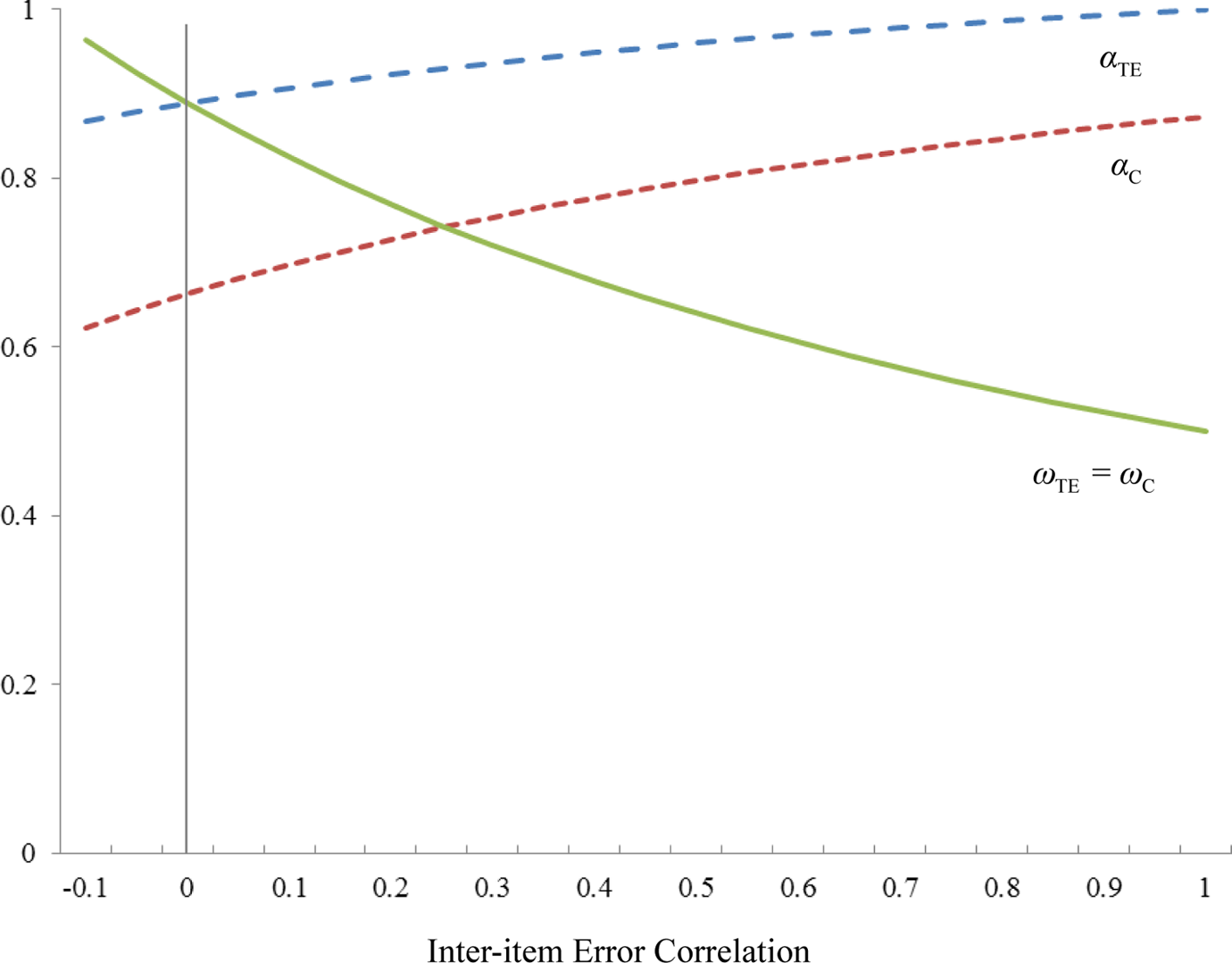
Figure 1 illustrates the differential effects of interitem error correlations on alpha and $ω$ , which were computed under the assumptions of unidimensionality and correlated item errors. A vertical line starting from correlation zero represents the condition of uncorrelated item errors, which is unrealistic and at best exceptional in an actual research environment. Alpha in the tau-equivalent condition, and the value of $ω$ has the same value as reliability, but alpha in the congeneric (but not tau-equivalent) condition underestimates reliability. As the interitem error correlation increases, the value of alpha in the two conditions also increases, but that of $ω$ decreases; the direction of these relations is the same as the reliability shown in Equation 10.

Figure 1.

Influence of interitem error correlation on $ω$ and $α$ .

Common Misconception: A High Value of Alpha Is an Indication of Internal Consistency

Alpha has a seemingly inextricable connection with internal consistency. Prestigious psychometricians refer to alpha as “a measure of internal consistency” (Nunnally & Bernstein, 1994, p. 290) or “an internal consistency estimate” (Thompson, 2003, p. 10). Popular textbooks on research methods offer more detailed descriptions of alpha, for example, “the most commonly reported index of internal consistency” (Christensen, Johnson, & Turner, 2011, p. 144) or “the most common and powerful method used today for calculating internal consistency reliability” (Rubin & Babbie, 2008, p. 184). The cognitive bond between the two terms is so strong that considerable empirical studies substitute the expression internal consistency for alpha when reporting reliability information (Hogan, Benjamin, & Brezinski, 2000).

Despite its frequent use, surprisingly little consensus exists about the precise meaning of internal consistency. This study identifies three different definitions of internal consistency that can be either explicitly or implicitly found in the literature: homogeneity, interrelatedness of a set of items, and general factor saturation.

When we consider the definitions of internal consistency, secondary or tertiary definition problems arise. The present study defines homogeneity as the unidimensionality of a set of items, based on previous studies (Cortina, 1993; Green, Lissitz, & Mulaik 1977; McDonald, 1981; Schmitt, 1996; Sijtsma, 2009a). Unidimensionality refers to the existence of one latent trait underlying a set of items (Hattie, 1985). The interrelatedness of a set of items is defined as the arithmetic mean of interitem correlation coefficients, that is, ${\overset{ˉ}{r}}_{i j}$ (Cronbach, 1951). General factor saturation refers to the proportion of test variance that is due to a general factor (Revelle & Zinbarg, 2009). The hierarchical omega ( $ω_{h}$ ) is the most recommended index of general factor saturation (Zinbarg et al., 2005).

The definition of internal consistency as homogeneity stems from Cronbach (1951), who used the two terms interchangeably (Schmitt, 1996). He also proposed that a high value of alpha is indicative of homogeneity. Green et al. (1977) and McDonald (1981) noted logical problems in the argument provided by Cronbach (1951), and other studies (e.g., Cortina, 1993; Schmitt, 1996; Ten Berge & Sočan, 2004) demonstrated that alpha cannot be an indication of homogeneity or unidimensionality by offering counterexamples. Nevertheless, such an interpretation persists (Green & Yang, 2009a).

The fact that alpha cannot evidence homogeneity may be demonstrated through another counterexample. Consider four tests, each consisting of eight items (V1–V8), whose observed variance-covariance matrices (A, B, C, and D) are presented in Table 1. Matrices A and B both illustrate test situations in which only a general factor is present and all items are homogeneous. Matrix C illustrates a situation in which no general factor exists but two group factors (one loaded on by V1–V4 and the other by V5–V8) are present. Matrix D represents a situation in which a general factor and two group factors are present. To avoid the confounding issue of specific factors and random errors, it is assumed that no specific factors exist. The two tests that are associated with matrices A and B are one-factor (i.e., homogeneous) tests, but they have different values of alpha—.7742 and .9492, respectively. This comparison indicates that the alpha value does not closely relate to test unidimensionality. Further, if we compute alpha values for matrices A and C, we obtain the same value of .7742, although matrix C is derived from a multidimensional test.

Table 1.

Four Variance-Covariance Matrices With Different Internal Structures.

A (a general factor only, less saturated)									B (a general factor only, more saturated)
	V1	V2	V3	V4	V5	V6	V7	V8		V1	V2	V3	V4	V5	V6	V7	V8
V1	1	.3	.3	.3	.3	.3	.3	.3	V1	1	.7	.7	.7	.7	.7	.7	.7
V2	.3	1	.3	.3	.3	.3	.3	.3	V2	.7	1	.7	.7	.7	.7	.7	.7
V3	.3	.3	1	.3	.3	.3	.3	.3	V3	.7	.7	1	.7	.7	.7	.7	.7
V4	.3	.3	.3	1	.3	.3	.3	.3	V4	.7	.7	.7	1	.7	.7	.7	.7
V5	.3	.3	.3	.3	1	.3	.3	.3	V5	.7	.7	.7	.7	1	.7	.7	.7
V6	.3	.3	.3	.3	.3	1	.3	.3	V6	.7	.7	.7	.7	.7	1	.7	.7
V7	.3	.3	.3	.3	.3	.3	1	.3	V7	.7	.7	.7	.7	.7	.7	1	.7
V8	.3	.3	.3	.3	.3	.3	.3	1	V8	.7	.7	.7	.7	.7	.7	.7	1
$ρ_{X X^{'}} \equiv ω = α = ω_{h} = .7742$ , ${\overset{ˉ}{r}}_{i j}$ = .3 ( $σ_{X}^{2} = 24.8$ , $1^{'} c c^{'} 1 = 19.2$ , $1^{'} A A^{'} 1 = 0$ )									$ρ_{X X^{'}} \equiv ω = α = ω_{h} = .9492$ , ${\overset{ˉ}{r}}_{i j}$ = .7 ( $σ_{X}^{2} = 47.2$ , $1^{'} c c^{'} 1 = 44.8$ , $1^{'} A A^{'} 1 = 0$ )
C (two group factors only)									D (a general factor and two group factors)
	V1	V2	V3	V4	V5	V6	V7	V8		V1	V2	V3	V4	V5	V6	V7	V8
V1	1	.7	.7	.7	0	0	0	0	V1	1	.7	.7	.7	.3	.3	.3	.3
V2	.7	1	.7	.7	0	0	0	0	V2	.7	1	.7	.7	.3	.3	.3	.3
V3	.7	.7	1	.7	0	0	0	0	V3	.7	.7	1	.7	.3	.3	.3	.3
V4	.7	.7	.7	1	0	0	0	0	V4	.7	.7	.7	1	.3	.3	.3	.3
V5	0	0	0	0	1	.7	.7	.7	V5	.3	.3	.3	.3	1	.7	.7	.7
V6	0	0	0	0	.7	1	.7	.7	V6	.3	.3	.3	.3	.7	1	.7	.7
V7	0	0	0	0	.7	.7	1	.7	V7	.3	.3	.3	.3	.7	.7	1	.7
V8	0	0	0	0	.7	.7	.7	1	V8	.3	.3	.3	.3	.7	.7	.7	1
$ρ_{X X^{'}} \equiv ω = .9032$ $α = .7742$ , $ω_{h} = 0$ , ${\overset{ˉ}{r}}_{i j}$ = .3 ( $σ_{X}^{2} = 24.8$ , $1^{'} c c^{'} 1 = 0$ , $1^{'} A A^{'} 1 = 22.4$ )									$ρ_{X X^{'}} \equiv ω = .9302$ $α = .8771$ , $ω_{h} = .5581$ , ${\overset{ˉ}{r}}_{i j}$ = .4714 ( $σ_{X}^{2} = 34.4$ , $1^{'} c c^{'} 1 = 19.2$ , $1^{'} A A^{'} 1 = 12.8$ )

The definition of internal consistency as the interrelatedness of a set of items has been accepted by many experts (Cortina, 1993; Green et al., 1977; McDonald, 1981; Schmitt, 1996; Sijtsma, 2009a). First, a high level of alpha does not indicate internal consistency in this definition. Alpha is a function of both item interrelatedness and the number of items in the set. Even when the average of interitem correlation coefficients is as low as .1, a satisfactory level of alpha can be obtained if there are a sufficient number of items (e.g., if $k =$ 21, $α$ = .7, where as if $k =$ 36, $α$ = .8). Therefore, we cannot make any conclusions about internal consistency solely based on the level of alpha.

Second, this definition is not congruent with the dictionary meaning of consistency in a situation in which strong group factors exist. According to the definition, we must declare that matrices A and C in Table 1 have the same level of internal consistency because they have the same value of ${\overset{ˉ}{r}}_{i j}$ . This conclusion conflicts with the observation that matrix C is not internally consistent in an everyday sense.

The definition of internal consistency as general factor saturation was suggested by Revelle (1979). A notable point about this definition is that alpha is no longer closely related to internal consistency when strong group factors and a weak general factor exist. In matrices A and C in Table 1, the same value of alpha exhibits a sharp contrast with $ω_{h}$ , which yields clearly distinguished values of .7742 and zero, respectively.

In summary, alpha does not indicate internal consistency in any definitions of psychometric properties. In addition, there is little utility in using the term internal consistency from the perspective of clarity and usefulness. What internal consistency exactly means is ambiguous. The use of more descriptive terms such as item interrelatedness is more helpful for understanding content and context.

Common Misconception: Reliability Will Always Be Improved by Deleting Items Using “Alpha if Item Deleted”

Equation 8 clearly illustrates that given the observed test score variance $σ_{X}^{2}$ , alpha is essentially a function of the number of items and the average interitem covariance. Theoretically, alpha increases as the number of items increases, with the average covariance being fixed. Peterson (1994) investigated the seemingly obvious relationship between the number of items and alpha and obtained the unexpected result that alpha does not significantly increase even if the number of items increases. Further, Peterson discovered that alpha increases as the number of items that are eliminated during scale development increases. This “paradox of the number of items” reveals two contrasting strategies that are commonly used to obtain an acceptable level of alpha. The first strategy is to increase the number of items to increase alpha, which overcomes problems with the quality of items by changing their quantity. The other strategy is to decrease the number of items. That is, the higher correlation between items is when the number of items is smaller may result from the selection of only higher correlating items, with lower correlating items being deleted. The “alpha if item deleted” information provided by statistical software packages facilitates the use of this strategy.

Kopalle and Lehmann (1997) suggested that deleting items with lower interitem correlations can lead to an overstatement of alpha, or “alpha inflation,” in which the sample-level alpha is more highly reported than the population-level alpha. They raised the need to separate the calibration sample, which determines the scale, and the cross-validation sample, which calculates reliability, and suggested that the deletion of items must follow a theoretical and logical basis.

Raykov (2007, 2008) revealed a more critical problem associated with reducing the number of items by the “alpha if item deleted” information. Raykov (2007) proposed that the actual reliability of a scale may decrease even though alpha appears to increase after the number of items is reduced, and Raykov (2008) proved that predictive validity can also decrease. Raykov (2008) proposed a latent variable modeling approach that produces point and interval estimates of criterion validity as well as reliability after the deletion of individual components. While Raykov (2008) raised the possibility that an increase in the sample-level value of alpha might be obtained at the expense of predictive validity, the potential tradeoff between reliability and content validity will be discussed in the next section.

We have no intention of discouraging the use of the “alpha if item deleted” function itself. It can be helpful for the identification and remedy of dysfunctional items within a scale. However, we generally discourage mechanical reliance on the output of statistical software. Researchers should be well versed in the substance of what they are studying and use that knowledge in conjunction with statistical indices to make judgments about the makeup of a measure.

Common Misconception: Alpha Should Be Greater Than or Equal to .7 (or, alternatively, .8)

The works of Nunnally (Nunnally, 1967, 1978; Nunnally & Bernstein, 1994) are the second most cited documents, with only the Bible having more citations. Interestingly, the broad-ranging remarks of Nunnally’s works across hundreds of pages are not cited nearly as often as their references to acceptable levels of alpha (.7 or .8). Nunnally most likely offered concrete numbers purely with the intention of providing his readers with some practical aid. Such advised levels create various problems, however.

First, the advised levels of alpha are neither the result of empirical research (Churchill & Peter, 1984; Peterson, 1994) nor the consequence of clear logical reasoning; instead, they were derived from Nunnally’s personal intuition. For example, there is no evidence that .7 is a better standard than .69 or .71.

Second, people use Nunnally’s authority as an immunity standard, which “legally” excuses them from having to think further about reliability when alpha values above .7 or .8 are obtained. There are two intriguing facts that demonstrate that Nunnally’s work (1967, 1978) is cited for its usefulness in providing a “hall pass” or “certificate” rather than for its content. First, in the first edition of the work, Nunnally (1967) stated that a reliability of .5 or .6 is sufficient for exploratory research; however, the standard applied to exploratory research was increased to .7 in the second edition (Nunnally, 1978). People choose which edition of Nunnally’s work to cite depending on whether their alpha is above or below .7 (Henson, 2001). Second, the second edition is still the most widely cited version of the work despite the existence of a third edition (Nunnally & Bernstein, 1994).

Third, the artificial effort to increase alpha above a certain level may harm reliability and validity. The strategy of deleting items by using the “alpha if item deleted” information to increase alpha may reduce both reliability (Raykov, 2007) and criterion validity (Raykov, 2008). Another common strategy to increase alpha is to repeatedly present slightly different items that essentially measure the same component of a particular construct. Each item must correctly represent its whole to obtain high content validity. Therefore, sacrificing the diversity of items to increase alpha hinders content validity. The phenomenon in which an increase in reliability is obtained at the cost of validity is also known as the attenuation paradox (Humphreys, 1956; Loevinger, 1954). This phenomenon is referred to as a paradox because a test with perfect reliability, despite seemingly being the epitome of an ideal test, is not valid. For example, all examinees who take a test with a reliability of unity will have either a score of zero or a perfect score, as an examinee who gives a correct/wrong answer to an item will also give correct/wrong answers to any other items. In a similar context, Streiner (2003) also argued that although a higher alpha is desirable, an excessively high level of alpha is not desirable because it accompanies unnecessary repetition and overlap.

Some scholars further argued that a high level of alpha is fundamentally undesirable. For example, Kline (1986) asserted that “high internal consistency can be … antithetical to high validity[;] … the importance of internal-consistency reliability has been exaggerated” (pp. 118-119). Boyle (1991) criticized researchers’ obsession with a high level of alpha, stating that “it may often be more appropriate to regard estimates such as the alpha coefficients as indicators of item redundancy and narrowness of a scale” (p. 291).

We recommend against mechanistically or automatically applying a cutoff criterion. When the importance of a decision made on the basis of a test score increases, the standard for reliability should also increase. Cortina’s (1993) advice that “the finer the distinction that needs to be made, the better the reliability must be” (p. 101) captures the essence of such a guideline. However, Lance, Butts, and Michels (2006) found that such a guideline is rarely followed; most empirical studies have used .70 as a universal standard of reliability regardless of the stage or purpose of research. One size does not fit all. The nature of the decision being made on the basis of a test should be the guide for the acceptable level of reliability.¹

Common Misconception: Alpha Is the Best Choice Among All Published Reliability Coefficients

Although alpha’s presence overwhelmingly overshadows many other reliability coefficients, McDonald (1981) claimed that “coefficient alpha cannot be used as a reliability coefficient” (p. 113). A number of reliability coefficients (i.e., estimators) have been proposed in an attempt to overcome the limitations of alpha, and several authors have compared the performance of these estimators. Osburn’s (2000) simulation study included 11 reliability coefficients and reported Max ( $λ_{4}$ ) as the most accurate estimator of reliability. Kamata, Turhan, and Darandari’s (2003) investigation of four methods revealed that stratified-alpha was the best alternative. In Revelle and Zinbarg’s (2009) analysis of 13 formulas, McDonald’s $ω$ was recommended as the best choice. The latent class reliability coefficient (LCRC) was ranked first in an analysis by van der Ark, van der Palm, and Sijtsma (2011), which considered five techniques. Tang and Cui’s (2012) comparison of three lower bounds supported the use of Guttman’s $λ_{2}$ .

In all of these studies, there was a common finding that alpha received relatively poor scores. A more striking fact is that five different reliability coefficients were ranked first by five comparison studies. The results of such studies give an impression that even among experts, there is no consensus on which methodology is superior to others. Until there is an explicit statement about which alternative method should replace alpha, users will continue to use it.

To overcome this situation, Sijtsma (2009a, p. 107) recommended the use of the greatest lower bound (glb) (Jackson & Agunwamba, 1977; Woodhouse & Jackson, 1977), declaring that his paper is “meant to invite debate on” the issue. His intention of stimulating debate was successfully realized; in 2009, four comments on his paper (Bentler, 2009; Green & Yang, 2009a, 2009b; Revelle & Zinbarg, 2009), as well as his rejoinder (Sijtsma, 2009b), were published in Psychometrika. However, the recommendation for the glb in Sijtsma (2009a) was not easily accepted. Revelle and Zinbarg (2009) criticized how the glb, unlike its name, yields a smaller value than McDonald’s $ω$ . Tang and Cui (2012) noted that the glb not only tends to yield an overestimation but also produces greater bias than $λ_{2}$ . Moreover, Sijtsma excluded the glb from a list of alternatives in a comparative study in which he participated (van der Ark et al., 2011).

Such reactions to Sijtsma (2009a) indicated what top psychometricians have been considering to be substitutes for alpha; all four comments proposed approaches based on SEM. Several authors have proposed methods for computing SEM estimates of reliability (Green & Yang, 2009b; Jöreskog, 1971; Miller, 1995; Raykov, 1997; Raykov & Shrout, 2002), including McDonald’s (1999) $ω$ , as shown in Equation 13. Alpha, which requires the more restrictive assumption of tau-equivalency, can be viewed as a special case of SEM estimators of reliability based on congeneric models. Alpha and SEM estimates have the same value if the similarity between items is tau-equivalent. Moreover, violation of the tau-equivalency assumption can be tested by using SEM procedures (Fleishman & Benson, 1987; Graham, 2006; Jöreskog & Sörbom, 1996; Miller, 1995).

A Framework for Choosing a Reliability Estimator

Examinations of the Assumptions of Unidimensionality and Tau-Equivalency

Alpha should no longer be an unconditional and automatic choice for reliability estimation. As Cortina (1993) noted and as our previous discussion suggests, alpha should be used for reliability estimation when the following conditions are met: (a) the test measures a single factor, (b) the test items are essentially tau-equivalent in statistical similarity, and (c) the error scores of the items are uncorrelated. However, all of these conditions are rarely met in practice; one or more of the assumptions regarding unidimensionality, essential tau-equivalency, and uncorrelated errors may be violated to some degree. This study does not devote further attention to the detection and correction of correlated errors; interested readers are referred to Kim and Feldt (2011) and Raykov (2004). Nevertheless, regarding the selection of a reliability estimator, we recommend that the assumption of unidimensionality and tau-equivalency be examined before the application of alpha and that SEM-based reliability estimators be substituted for alpha when one of these conditions is not satisfied. Figure 2 summarizes our guidelines.

Figure 2.

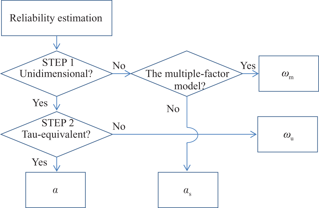
A framework for choosing a reliability estimator.

Unidimensionality

While various methods have been developed to test unidimensionality (Hattie, 1985), this study focuses on SEM approaches. The unidimensional model is nested within the multidimensional model in SEM, and the chi-square difference is usually used to test for statistical significance. Three models can be employed to conceptualize multidimensionality in SEM: the correlated factors model, the higher-order factor model, and the multiple-factor model (Figure 3).

Figure 3.

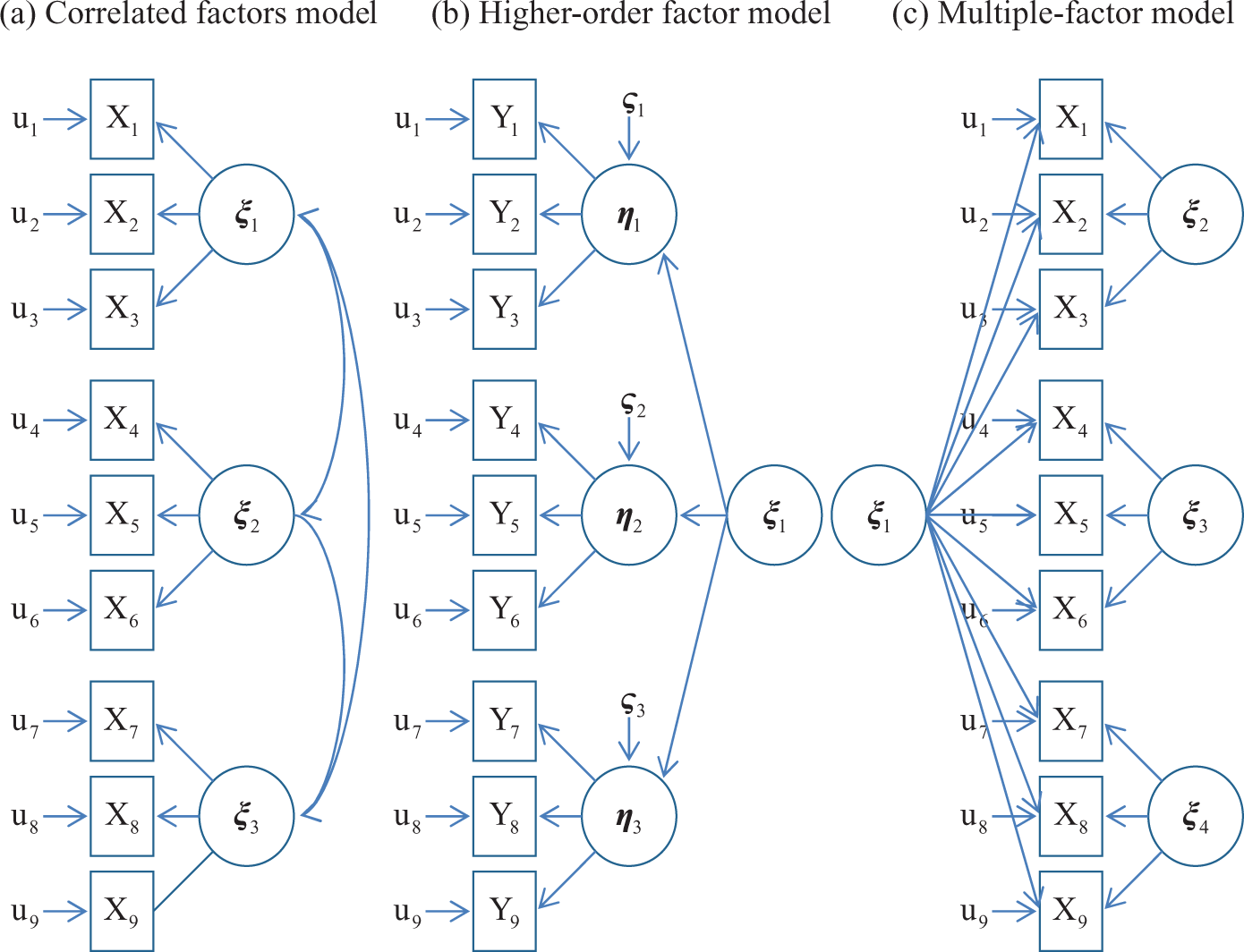
Three models of multidimensionality in structural equation modeling.

Although the correlated factors model is most frequently used among organizational researchers, its popularity is not an indication of its superiority. As the exact opposite of the unidimensional model, the correlated factors model includes only subdomain constructs and omits a common construct, which is a hidden influencer that causes the latent variables to correlate with each other. Moreover, paradoxically, the construct that most scale developers originally design to measure (Reise, 2012) and that most researchers primarily intend to study is excluded from the measurement model.

The higher-order factor model and the multiple-factor model, also known as the hierarchical factor model or bifactor model, share a commonality; they consider both subdomain factors and a common factor. While a general factor (i.e., $ξ_{1}$ in the multiple-factor model of Figure 3) is analogous to a second-order factor (i.e., $ξ_{1}$ in the higher-order factor model), group factors (i.e., $ξ_{2}$ – $ξ_{4}$ in the multiple-factor model) are not analogous to first-order factors (i.e., $η_{i}$ ). Group factors are analogous to disturbances (i.e., $ς_{i}$ ), as both are orthogonal to a general/second-order factor and both explain the variances that were not explained by this factor (Reise, Moore, & Haviland, 2010). The two models are mathematically equivalent under some conditions (Yung, Thissen, & McLeod, 1999).

The two models nevertheless have some interesting differences. While a higher-order factor subjugates the lower-order factors, a general factor competes with the group factors in explaining the variances of the manifest variables. Whereas a general factor is directly linked with the manifest variables, a higher-order factor’s connections with the manifest variables must be mediated by the lower-order factors (Reise et al., 2010).

Although the multiple-factor model is the least understood and least used model by organizational researchers, it has several advantages over the higher-order factor model (Chen, West, & Sousa, 2006). Multiple-factor models can easily detect a nonexistent domain-specific factor because such a factor will cause an identification problem and a nonsignificant factor loading for the group factor; however, higher-order factor models are insensitive to signal such anomalies because nonsignificant variances of the disturbances of lower-order factors usually do not cause any estimation problems and can be easily overlooked by researchers. While group factors can be predicted by external variables independently of the general factor, estimating paths between the disturbances of first-order factors and external variables is difficult with second-order factor models. Because the higher-order model is nested within the multiple-factor model (Yung et al., 1999), the multiple-factor model functions as a baseline model for testing whether the chi-square differences between the models are statistically significant (Chen et al., 2006).

Let us describe the typical constraints of the multiple-factor model. Every manifest variable is assumed to have one general factor and one (and only one) group factor. A general factor is orthogonal to or uncorrelated with group factors by definition. Group factors are also generally constrained to be orthogonal to or uncorrelated with each other for identification and interpretability (Reise, 2012). In other words, the variance-covariance matrix of the latent variables (i.e., $Φ$ ) is usually restricted to a diagonal matrix (i.e., all off-diagonal elements or covariances are fixed at zero) or an identity matrix (i.e., all off-diagonal elements or covariances are fixed at zero and the variances of the latent variables are fixed at 1.0).

Tau-Equivalency

More restrictions are placed on the tau-equivalent model than on the congeneric model. In the latter model, either the variance of the latent variable or a factor loading of one of the manifest variables must be fixed at a non-zero value (typically 1.0) to determine the scale of the latent variable. The former model adds the constraint of equal factor loadings (i.e., $λ_{i} = λ_{j}$ ) to those of the latter model and thus requires that one of the following conditions be met: (a) the variance of the latent variable is fixed at a non-zero value and every factor loading of the manifest variables that measure a common latent variable is constrained to be equal or (b) every factor loading of the manifest variables that measure a common latent variable is fixed at an equal non-zero value. Figure 4 summarizes these requirements. Because the tau-equivalent model is nested within the congeneric model, the chi-square difference between the two models can be used to test for statistical significance.

Figure 4.

The tau-equivalent model and the congeneric model in structural equation modeling.

Reliability Estimators for Multidimensional Data

Among the statistical procedures that have been presented for estimating the reliability of multidimensional test scores, two estimators can be recommended for organizational researchers: the multidimensional version of $ω$ (hereinafter referred to as $ω_{m}$ ) and stratified-alpha (hereinafter referred to as $α_{s}$ ).

$ω_{m}$

This study offers formulas and computation examples of $ω_{m}$ that are accessible to those who are not very familiar with matrix notation. Previous studies that have reported the formulas of the omega coefficients have typically only briefly referenced matrix formulas, as we did in Equations 13 and 14. Basically, $ω_{m}$ is an SEM-based reliability estimator, and the value of $ω_{m}$ is computed by fitting a multiple-factor measurement model to observed data. Equation 15 shows a computation-saving formula of ${\hat{ω}}_{m}$ , and Equation 16 displays another algebraically equivalent formula. That is,

{\hat{ω}}_{m} = 1 - \frac{\sum_{i = 1}^{k} {\hat{σ}}_{u_{i}}^{2}}{{\hat{σ}}_{X}^{2}}, o r

{\hat{ω}}_{m} = \frac{{(\sum_{i = 1}^{k} {\hat{λ}}_{i 1})}^{2} + \sum_{j = 2}^{r + 1} {(\sum_{i = 1}^{k} {\hat{λ}}_{i j})}^{2}}{{\hat{σ}}_{X}^{2}},

where ${\hat{λ}}_{i 1}$ is the estimated unstandardized factor loading of item $i$ on a general factor, ${\hat{λ}}_{i j}$ is the estimated unstandardized factor loading of item $i$ on the $(j - 1)$ th group factor, $r$ is the number of group factors, ${\hat{σ}}_{u_{i}}^{2}$ is the estimated unique variance of item $i$ , and ${\hat{σ}}_{X}^{2}$ is the sum of all components in a fitted/reproduced variance-covariance matrix.

Let us consider an illustrative example. If we apply the orthogonal factor solutions to the matrix D data in Table 1, we will obtain ${\hat{λ}}_{i 1}$ = $\sqrt{.3}$ ( $i = 1, \dots, 8$ ), ${\hat{λ}}_{i 2}$ = $\sqrt{.4}$ ( $i = 1, \dots, 4$ ), ${\hat{λ}}_{i 2}$ =0 ( $i = 5, \dots, 8$ ), ${\hat{λ}}_{i 3}$ =0 ( $i = 1, \dots, 4$ ), and ${\hat{λ}}_{i 3}$ = $\sqrt{.4}$ ( $i = 5, \dots, 8$ ), and ${\hat{σ}}_{u_{i}}^{2}$ =.3 for all items. These estimates lead to ${(\sum_{i = 1}^{k} {\hat{λ}}_{i 1})}^{2}$ + $\sum_{j = 2}^{3} {(\sum_{i = 1}^{k} {\hat{λ}}_{i j})}^{2}$ = 8²(.3) + [4²(.4) + 4²(.4)] = 19.2 + 12.8 = 32, $\sum_{i = 1}^{8} {\hat{σ}}_{u_{i}}^{2}$ = 8(.3) = 2.4, and ${\hat{σ}}_{X}^{2}$ =34.4. Finally, we obtain the estimate of ${\hat{ω}}_{m}$ =1 – (2.4/34.4) = .9302, according to Equation 15.

Stratified Alpha ( $α_{s}$ )

Our plan B is to use $α_{s}$ if the SEM approach fails. Not all multidimensional data fit the multiple-factor model nicely. It requires well-structured group factors to be properly estimated (Reise, 2012). For example, as we previously discussed, the existence of a trivial group factor is likely to cause identification and estimation problems (Chen et al., 2006). $α_{s}$ is an easy-to-use alternative that is applicable to a case in which the model-based reliability estimator is not very successful. Recall that Kamata et al.’s (2003) performance comparison reported $α_{s}$ as the best method.

To address the score reliability of stratified tests, Rajaratnam, Cronbach, and Gleser (1965) derived $α_{s}$ from generalizability theory as

α_{s} = 1 - \frac{\sum_{i = 1}^{k} σ_{X_{i}}^{2} (1 - α_{i})}{σ_{X}^{2}},

where $α_{i}$ each are alpha coefficients for scores of item $i$ . This formula of stratified alpha entails the following estimation procedure: (a) obtain observed score (unbiased) variance ${\hat{σ}}_{X_{i}}^{2}$ and coefficient alpha ${\hat{α}}_{i}$ for each item, (b) estimate error variance by using the formula ${\hat{σ}}_{e_{i}}^{2} = {\hat{σ}}_{X_{i}}^{2} (1 - {\hat{α}}_{i})$ for each item, and then (c) substitute the summed error variance and the total observed variance ${\hat{σ}}_{X}^{2}$ into the formula of $α_{s}$ .

Let us illustrate the $α_{s}$ estimation procedure with the matrix D data in Table 1, for which the first and second part-tests include the set of items V1–V4 and the set of items V5–V8, respectively. We can figure out that ${\hat{σ}}_{x}^{2}$ = 12.4 and that ${\hat{α}}_{i}$ = .9032 (thus ${\hat{σ}}_{e_{i}}^{2}$ = 1.2) for both part-tests. Substitution of these component values into Equation 17 leads to ${\hat{α}}_{s} = 1 - (2.4 / 34.4) = .9302$ . Notice that ${\hat{α}}_{s} = {\hat{ω}}_{m}$ for the matrix D data.

Reliability Estimators Based on the Congeneric Measurement Model

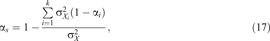
When the tau-equivalency assumption is violated, an SEM-based congeneric reliability estimator is recommended as an alternative to coefficient alpha. The SEM-based congeneric reliability, presented by Jöreskog (1971) and McDonald (1999, p. 89), is simply the unidimensional version of $ω$ (hereinafter referred to as $ω_{u}$ ) with the one common factor $ξ$ and thus can be expressed as

ω_{u} = \frac{1^{'} λ σ_{ξ}^{2} λ^{'} 1}{1^{'} Σ_{x} 1} = \frac{{(\sum λ_{i})}^{2} σ_{ξ}^{2}}{{(\sum λ_{i})}^{2} σ_{ξ}^{2} + \sum σ_{u_{i}}^{2}},

which is numerically equal to Equation 14. The estimate of $ω_{u}$ is obtained by fitting the congeneric measurement model to sample data and substituting the estimates of the SEM parameters ( $λ_{i}$ and $σ_{u_{i}}^{2}$ ) into Equation 18. When the SEM parameters are estimated, the value of $σ_{ξ}^{2}$ is usually set at 1.0 to solve scale indeterminacy. Thus, in the literature, the estimate of $ω_{u}$ is often expressed as Equation 19. Equation 20 shows two other algebraically equivalent formulas of ${\hat{ω}}_{u}$ . That is,

{\hat{ω}}_{u} = \frac{{(\sum {\hat{λ}}_{i})}^{2}}{{(\sum {\hat{λ}}_{i})}^{2} + \sum {\hat{σ}}_{u_{i}}^{2}},

{\hat{ω}}_{u} = \frac{{(\sum {\hat{λ}}_{i})}^{2}}{{\hat{σ}}_{X}^{2}} = 1 - \frac{\sum {\hat{σ}}_{u_{i}}^{2}}{{\hat{σ}}_{X}^{2}} .

Organizational researchers usually refer to these formulas as “composite reliability” (Peterson & Kim, 2013), which is supposedly a shorthand for the reliability of composite scores. This designation is a misnomer, however, because the dictionary meaning of the term is too general to be limited to a specific method, and it can encompass broad categories of reliability estimators, including alpha. Using such a designation is similar to calling a proper noun (e.g., Chicago) by a common noun (e.g., city). Composite reliability is commonly abbreviated to CR. If this acronym should be used, the term congeneric reliability describes the characteristics of this reliability coefficient better than composite reliability or construct reliability do.

Examples of the Computation of Omega Coefficients

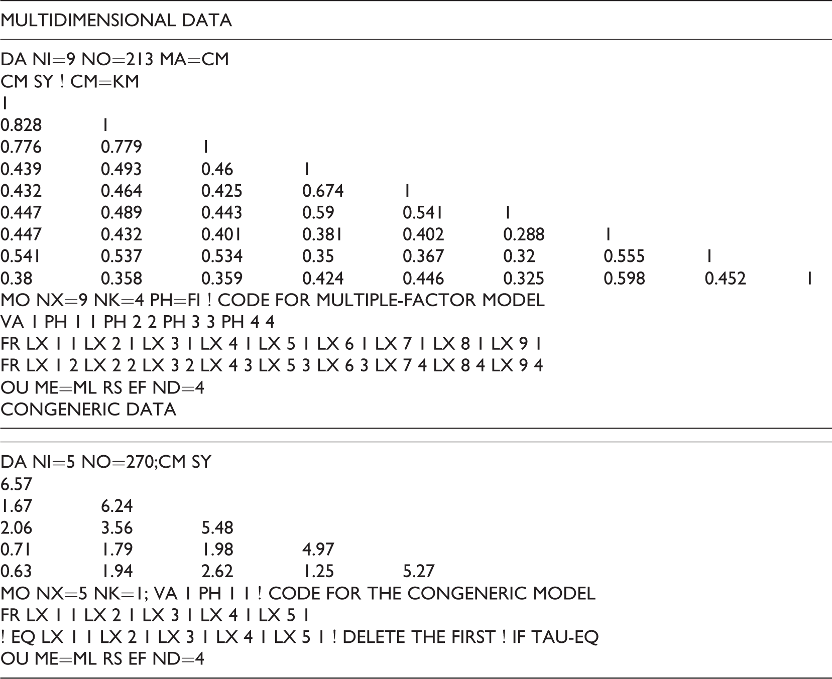
This section offers two examples that allow interested readers to replicate our computations.² Readers who are familiar with R, a free open-source statistical software platform, will consider the psych package (Revelle, 2014) to be the most convenient tool for obtaining omega coefficients because its Omega function estimates them spontaneously. We will assume that our typical readers use one of the SEM packages (e.g., LISREL, Mplus, and AMOS) that do not offer automated calculations of omega coefficients. Our LISREL program codes are displayed in Appendix 2.

Table 2 presents an examination of the assumption of unidimensionality. The fit indices for the unidimensional model indicate unacceptable fit, suggesting that more than one latent trait is underlying this set of items. The chi-square difference between the unidimensional model and the multiple-factor model is significant at $α = .05$ , and $ω_{m}$ is recommended as the proper reliability estimator for the data, according to the guidelines shown in Figure 2. Although the higher-order factor model is not necessary for a unidimensionality check, we included it because we compared it with the multiple-factor model in the previous section. The chi-square difference between the two models is significant at $α = .05$ , consistent with Chen et al.’s (2006) findings that the multiple-factor model usually has greater power than the higher-order factor model.

Table 2.

An Examination of the Unidimensionality Assumption.

	CFI	TLI	RMSEA	df	$χ^{2}$	p
a. Unidimensional	.80	.74	.21	27	233.54	.00
b. Higher-order factor	.98	.98	.05	24	38.19	.03
c. Multiple-factor	.99	.98	.03	18	24.21	.14
Difference (a – c)				9	209.32	.00
Difference (b – c)				6	13.98	.02

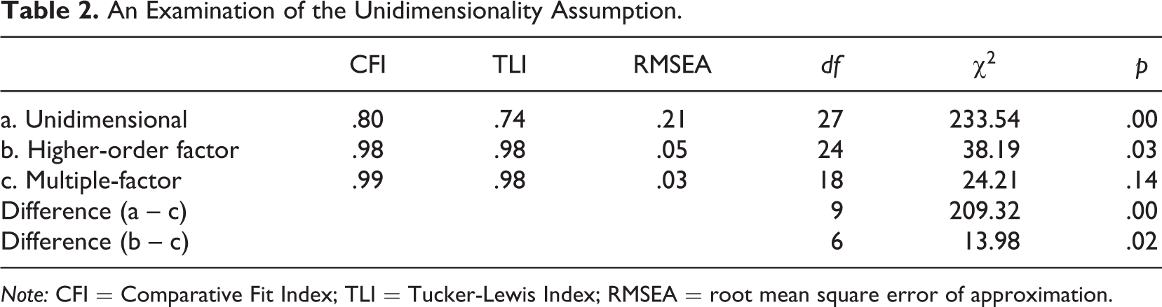
Note: CFI = Comparative Fit Index; TLI = Tucker-Lewis Index; RMSEA = root mean square error of approximation.

Table 3 displays a step-by-step explanation of the computation of ${\hat{ω}}_{m}$ . STEP 1 is to sum the unique variances; the use of a spreadsheet program facilitates this process. STEP 2 is to sum the fitted/implied covariance matrix. Most SEM packages present only lower triangular and diagonal elements of the fitted covariance matrix rather than full elements of the matrix. We can obtain the sum of all the elements by using the formula $2 (\sum (s u b d i a g o n a l) + \sum (d i a g o n a l)) - \sum (d i a g o n a l)$ . STEP 3 is to compute ${\hat{ω}}_{m}$ ; the value of ${\hat{ω}}_{m}$ for these data is .9312, according to Equation 15. We used the sample covariance matrix to compute the values of $\hat{α}$ and ${\hat{α}}_{s}$ and obtained .8915 and .9260, respectively.

Table 3.

A Computation of ${\hat{ω}}_{m}$ for a Multidimensional Data Example.

STEP 1: Sum the Unique Variances		STEP 2: Sum the Fitted/Implied Covariance Matrix
	${\hat{σ}}_{u_{i}}^{2}$	X1	X2	X3	X4	X5	X6	X7	X8	X9
X1	0.17	1.00
X2	0.17	0.83	1.00
X3	0.27	0.78	0.78	1.00
X4	0.25	0.47	0.48	0.46	1.00
X5	0.39	0.46	0.47	0.45	0.67	1.00
X6	0.52	0.44	0.45	0.43	0.59	0.54	1.00
X7	0.15	0.44	0.45	0.43	0.34	0.34	0.32	1.00
X8	0.50	0.51	0.52	0.50	0.40	0.40	0.38	0.56	1.00
X9	0.55	0.41	0.42	0.40	0.32	0.32	0.30	0.60	0.45	1.00
$\sum$	2.97	$2 (\sum (s u b d i a g o n a l) + \sum (d i a g o n a l)) - \sum (d i a g o n a l)$ = 43.20
STEP 3: Compute ${\hat{ω}}_{m}$		${\hat{ω}}_{m}$ = 1 – 2.97 / 43.20 = .9312

Table 4 presents an examination of the assumption of tau-equivalency. The fit indices for the tau-equivalent model indicate poor fit, and its chi-square value is significantly greater than that of the congeneric model at $α = .05$ . According to our guidelines in Figure 2, $ω_{u}$ is recommended for the data.

Table 4.

An Examination of the Tau-Equivalency Assumption.

	CFI	TLI	RMSEA	df	$χ^{2}$	p
a. Tau-equivalent	.79	.77	.14	9	64.64	.00
b. Congeneric	1.00	1.00	.01	5	5.21	.39
Difference (a – b)				4	59.43	.00

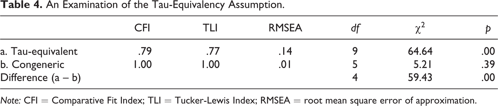
Note: CFI = Comparative Fit Index; TLI = Tucker-Lewis Index; RMSEA = root mean square error of approximation.

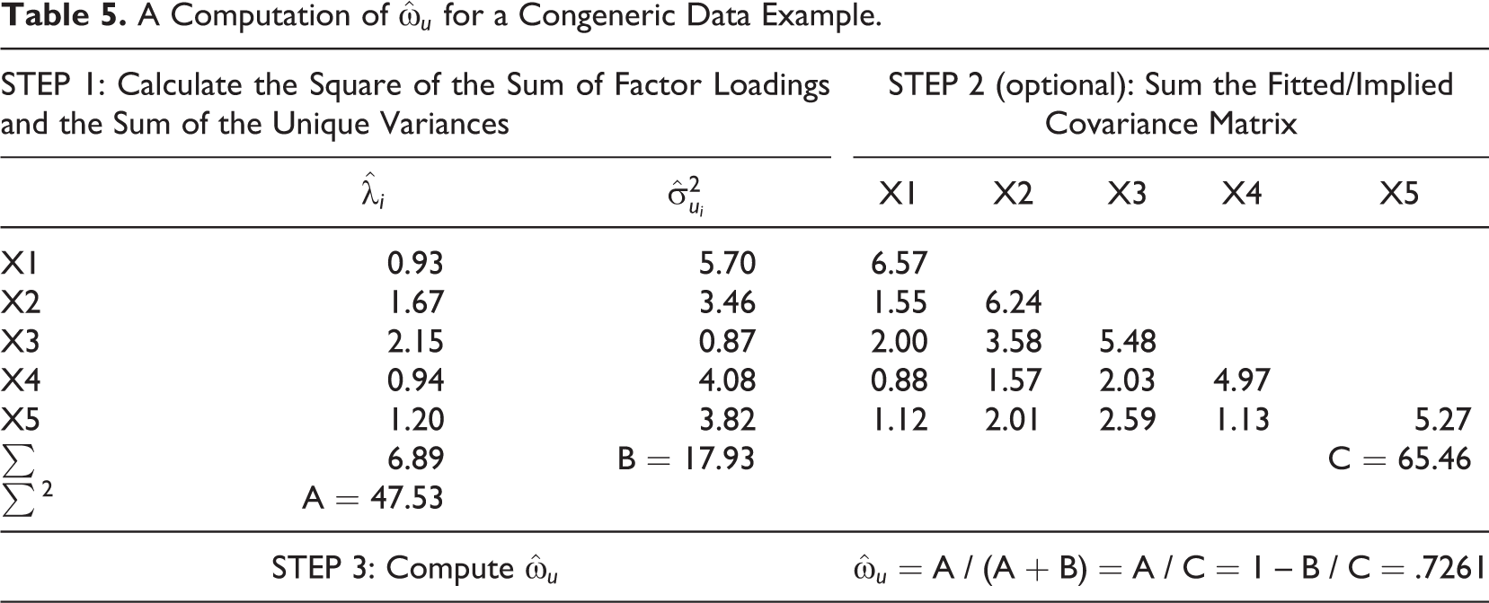
Table 5 displays the computation of ${\hat{ω}}_{u}$ . STEP 1 is to calculate the square of the sum of factor loadings and the sum of the unique variances. We can skip STEP 2 if we apply the computation-saving formula in Equation 19. In STEP 3, we can use any one of three equivalent formulas, all of which produce the same value of .7261. The value of $\hat{α}$ is .7009 for the data.

Table 5.

A Computation of ${\hat{ω}}_{u}$ for a Congeneric Data Example.

STEP 1: Calculate the Square of the Sum of Factor Loadings and the Sum of the Unique Variances			STEP 2 (optional): Sum the Fitted/Implied Covariance Matrix
	${\hat{λ}}_{i}$	${\hat{σ}}_{u_{i}}^{2}$	X1	X2	X3	X4	X5
X1	0.93	5.70	6.57
X2	1.67	3.46	1.55	6.24
X3	2.15	0.87	2.00	3.58	5.48
X4	0.94	4.08	0.88	1.57	2.03	4.97
X5	1.20	3.82	1.12	2.01	2.59	1.13	5.27
$\sum$	6.89	B = 17.93					C = 65.46
$\sum^{2}$	A = 47.53
STEP 3: Compute ${\hat{ω}}_{u}$			${\hat{ω}}_{u}$ = A / (A + B) = A / C = 1 – B / C = .7261

Conclusion

We commonly observe cases in which the best-selling products are not the products with the best quality. When the switching cost is higher, consumers tend to choose a more familiar alternative (e.g., the QWERTY keyboard layout) even though they know of a more efficient alternative (e.g., the Dvorak keyboard layout). Because of network externalities, in which other people’s choices affect the utility of an individual, in some situations, the winner may take all. For example, an individual may face a considerable disadvantage if he or she uses a different spreadsheet program while everyone else uses Microsoft Excel.

Alpha is a good example of how such marketing concepts may be applied to the choice of statistical analysis methods. Alpha is a relatively inferior method despite its widespread use. Even if users are aware of alpha’s inferiority, they may be unwilling to invest effort into becoming familiar with other reliability coefficients. Moreover, although they may be willing to tolerate personal costs from switching to another reliability coefficient, they may fear penalties incurred from not using the alpha coefficient in their studies because dissertation committees and editors are likely familiar with alpha but may not be familiar with its alternatives. In the perspective of network externality, substituting alpha with a superior alternative is not merely a matter of personal choice but a matter of academia consciously responding to the issue. It would be prudent for the editors of various academic journals on organizational research to recommend that their contributors use superior alternatives with or in place of alpha in their works.

Footnotes

Appendix 1

The computation uses Lucke’s (2005, p. 117) compound symmetric item error covariance model, which requires errors to be equally correlated among items. The item error variances are $θ^{2}$ , the item error correlations are $γ$ , the number of items is $k$ , the deviance from tau-equivalency for test i is $δ_{i}$ , and the average of factor loadings is $\overset{ˉ}{λ}$ . $α$ and $ω$ are shown in the following:

Note that $α$ is a monotonically increasing function of $γ$ because k(k −1) $θ^{2}$ in the numerator is greater than (k − 1)(k −1) $θ^{2}$ in the denominator, while $ω$ is a monotonically decreasing function of $γ$ . Note also that $α$ and $ω$ have the same value of $k {\overset{ˉ}{λ}}^{2} / k {\overset{ˉ}{λ}}^{2} + θ^{2})$ if $δ = 0$ (i.e., tau-equivalent) and $γ = 0$ (i.e., uncorrelated errors). We consider a set of two hypothetical tests (X_TE and X_C), each with $k$ = 8 items, $\overset{ˉ}{λ}$ = 3, and $θ^{2}$ = 9 but with different vectors of factor loadings. These conditions are similar to those of Lucke (2005, p. 119), except for $k$ .

X_TE with $λ_{T E} = {[3, 3, 3, 3, 3, 3, 3, 3]}^{'}$ so that $δ_{T E} = 0$ .

X_C with $λ_{C} = {[- 1, - 1, - 1, - 1, 7, 7, 7, 7]}^{'}$ so that $δ_{C} = 128$ .

The values of $α$ and $ω$ in our hypothetical data can be expressed as in the following:

α = \frac{8 \times 7 \times (3^{2} + 9 γ) - δ}{(7) \{8 \times 3^{2} + [1 + 7 γ] \times 9\}}; ω = \frac{8 \times 3^{2}}{8 \times 3^{2} + [1 + 7 γ] \times 9}

Appendix 2

MULTIDIMENSIONAL DATA
DA NI=9 NO=213 MA=CM
CM SY ! CM=KM
1
0.828	1
0.776	0.779	1
0.439	0.493	0.46	1
0.432	0.464	0.425	0.674	1
0.447	0.489	0.443	0.59	0.541	1
0.447	0.432	0.401	0.381	0.402	0.288	1
0.541	0.537	0.534	0.35	0.367	0.32	0.555	1
0.38	0.358	0.359	0.424	0.446	0.325	0.598	0.452	1
MO NX=9 NK=4 PH=FI ! CODE FOR MULTIPLE-FACTOR MODEL
VA 1 PH 1 1 PH 2 2 PH 3 3 PH 4 4
FR LX 1 1 LX 2 1 LX 3 1 LX 4 1 LX 5 1 LX 6 1 LX 7 1 LX 8 1 LX 9 1
FR LX 1 2 LX 2 2 LX 3 2 LX 4 3 LX 5 3 LX 6 3 LX 7 4 LX 8 4 LX 9 4
OU ME=ML RS EF ND=4
CONGENERIC DATA
DA NI=5 NO=270;CM SY
6.57
1.67	6.24
2.06	3.56	5.48
0.71	1.79	1.98	4.97
0.63	1.94	2.62	1.25	5.27
MO NX=5 NK=1; VA 1 PH 1 1 ! CODE FOR THE CONGENERIC MODEL
FR LX 1 1 LX 2 1 LX 3 1 LX 4 1 LX 5 1
! EQ LX 1 1 LX 2 1 LX 3 1 LX 4 1 LX 5 1 ! DELETE THE FIRST ! IF TAU-EQ
OU ME=ML RS EF ND=4

Acknowledgments

The authors are deeply grateful to Professor Meade and the two anonymous ORM reviewers for their invaluable guidance and constructive comments. They also acknowledge the support provided by Kyung Su Liu.

Declaration of Conflicting Interests

The author(s) declared no potential conflicts of interest with respect to the research, authorship, and/or publication of this article.

Funding

The author(s) disclosed receipt of the following financial support for the research, authorship and/or publication of this article: The present research has been conducted by the Research Grant of Kwangwoon University in 2014.

Notes

References

Bentler

P. M.

(2009). Alpha, dimension-free, and model-based internal consistency reliability. Psychometrika, 74 (1), 137–143.

Boyle

G. J.

(1991). Does item homogeneity indicate internal consistency or item redundancy in psychometric scales? Personality & Individual Differences, 12 (3), 291–294.

Brown

(1910). Some experimental results in the correlation of mental abilities. British Journal of Psychology, 3 (3), 296–322.

Chen

F. F.

West

S. G.

Sousa

K. H.

(2006). A comparison of bifactor and second-order models of quality of life. Multivariate Behavioral Research, 41 (2), 189–225.

Christensen

L. B.

Johnson

R. B.

Turner

L. A.

(2011). Research methods, design, and analysis (11th ed.). Boston, MA: Pearson.

Churchill

G. A.

Peter

J. P.

(1984). Research design effects on the reliability of rating scales: A meta-analysis. Journal of Marketing Research, 21, 360–375.

Cortina

J. M.

(1993). What is coefficient alpha? An examination of theory and applications. Journal of Applied Psychology, 78 (1), 98–104.

Cronbach

L. J.

(1951). Coefficient alpha and the internal structure of tests. Psychometrika, 16 (3), 297–334.

Cronbach

L. J.

(2004). My current thoughts on coefficient alpha and successor procedures. Educational and Psychological Measurement, 64 (3), 391–418.

10.

Cronbach

L. J.

Hartmann

(1954). A note on negative reliabilities. Educational and Psychological Measurement, 14 (2), 342–346.

11.

Feldt

L. S.

Brennan

R. L.

(1989). Reliability. In Linn

R. L.

(Ed.), Educational measurement (3rd ed., pp. 105–146). New York, NY: American Council on Education and Macmillan.

12.

Flanagan

J. C.

(1937). A proposed procedure for increasing the efficiency of objective tests. Journal of Educational Psychology, 28 (1), 17–21.

13.

Fleishman

Benson

(1987). Using LISREL to evaluate measurement models and scale reliability. Educational and Psychological Measurement, 47 (4), 925–939.

14.

Graham

J. M.

(2006). Congeneric and (essentially) tau-equivalent estimates of score reliability: What they are and how to use them. Educational and Psychological Measurement, 66 (6), 930–944.

15.

Green

S. B.

Lissitz

R. W.

Mulaik

S. A.

(1977). Limitations of coefficient alpha as an index of test unidimensionality. Educational and Psychological Measurement, 37 (4), 827–838.

16.

Green

S. B.

Yang

(2009a). Commentary on coefficient alpha: A cautionary tale. Psychometrika, 74 (1), 121–135.

17.

Green

S. B.

Yang

(2009b). Reliability of summed item scores using structural equation modeling: An alternative to coefficient alpha. Psychometrika, 74 (1), 155–167.

18.

Guttman

(1945). A basis for analyzing test-retest reliability. Psychometrika, 10 (4), 255–282.

19.

Haertel

E. H.

(2006). Reliability. In Brennan

R. L.

(Ed.), Educational measurement (4th ed., pp. 65–110). Westport, CT: American Council on Education and Praeger.

20.

Harzing

A.W.

(2013). Publish or perish. Retrieved from http://www.harzing.com/pop.htm

21.

Hattie

(1985). Assessing unidimensionality of tests and items. Applied Psychological Measurement, 9 (2), 139–164.

22.

Henson

R. K.

(2001). Understanding internal consistency reliability estimates: A conceptual primer on coefficient alpha. Measurement and Evaluation in Counseling and Development, 34 (3), 177–189.

23.

Hogan

T. P.

Benjamin

Brezinski

K. L.

(2000). Reliability methods: A note on the frequency of use of various types. Educational and Psychological Measurement, 60 (4), 523–531.

24.

Hoyt

(1941). Test reliability estimated by analysis of variance. Psychometrika, 6 (3), 153–160.

25.

Humphreys

(1956). The normal curve and the attenuation paradox in test theory. Psychological Bulletin, 53 (6), 472–476.

26.

Jackson

P. H.

Agunwamba

C. C.

(1977). Lower bounds for the reliability of the total score on a test composed of non-homogeneous items: I: Algebraic lower bounds. Psychometrika, 42 (4), 567–578.

27.

Jöreskog

K. G.

(1971). Statistical analysis of sets of congeneric tests. Psychometrika, 36 (2), 109–133.

28.

Jöreskog

K. G.

Sörbom

(1996). LISREL 8: User’s reference guide (2nd ed.). Chicago, IL: Scientific Software International.

29.

Kamata

Turhan

Darandari

(2003). Estimating reliability for multidimensional composite scale scores. Paper presented at the annual meeting of American Educational Research Association, Chicago.

30.

Kim

Feldt

L. S.

(2011). A comparative study on coefficient alpha and congeneric-model-based reliability estimators for tests composed of clusters of items. Journal of Educational Evaluation, 24 (4), 1061–1084.

31.

Kline

(1986). A handbook of test construction: Introduction to psychometric design. London: Methuen.

32.

Kopalle

P. K.

Lehmann

D. R.

(1997). Alpha inflation? The impact of eliminating scale items on Cronbach’s alpha. Organizational Behavior and Human Decision Processes, 70 (3), 189–197.

33.

Kuder

G. F.

Richardson

M. W.

(1937). The theory of the estimation of test reliability. Psychometrika, 2 (3), 151–160.

34.

Lance

C. E.

Butts

M. M.

Michels

L. C.

(2006). The sources of four commonly reported cutoff criteria. Organizational Research Methods, 9 (2), 202–220.

35.

Loevinger

(1954). The attenuation paradox in test theory. Psychological Bulletin, 51 (5), 493–504.

36.

Lord

F. M.

Novick

M. R.

(1968). Statistical theories of mental test scores. Reading, MA: Addison-Wesley.

37.

Lucke

J. F.

(2005). “Rassling the hog”: The influence of correlated item error on internal consistency, classical reliability and congeneric reliability. Applied Psychological Measurement, 29(2), 106–125.

38.

McDonald

R. P.

(1970). The theoretical foundations of common factor analysis, principal factor analysis, and alpha factor analysis. British Journal of Mathematical and Statistical Psychology, 23 (1), 1–21.

39.

McDonald

R. P.

(1981). The dimensionality of tests and items. British Journal of Mathematical and Statistical Psychology, 34 (1), 100–117.

40.

McDonald

R. P.

(1999). Test theory: A unified treatment. Mahwah, NJ: Lawrence Erlbaum.

41.

Miller

M. B.

(1995). Coefficient alpha: A basic introduction from the perspectives of classical test theory and structural equation modeling. Structural Equation Modeling, 2 (3), 255–273.

42.

Mosier

C. I.

(1941). A short cut in the estimation of split-halves coefficients. Educational and Psychological Measurement, 1 (1), 407–408.

43.

Novick

M. R.

Lewis

(1967). Coefficient alpha and the reliability of composite measurements. Psychometrika, 32 (1), 1–13.

44.

Nunnally

J. C.

(1967). Psychometric theory. New York, NY: McGraw-Hill.

45.

Nunnally

J. C.

(1978). Psychometric theory (2nd ed.). New York, NY: McGraw-Hill.

46.

Nunnally

J. C.

Bernstein

I. H.

(1994). Psychometric theory (3rd ed.). New York, NY: McGraw-Hill.

47.

Osburn

H. G.

(2000). Coefficient alpha and related internal consistency reliability coefficients. Psychological Methods, 5 (3), 343–355.

48.

Peterson

R. A.

(1994). A meta-analysis of Cronbach’s coefficient alpha. Journal of Consumer Research, 21, 381–391.

49.

Peterson

R. A.

Kim

(2013). On the relationship between coefficient alpha and composite reliability. Journal of Applied Psychology, 98 (1), 194–198.

50.

Rajaratnam

Cronbach

L. J.

Gleser

G. C.

(1965). Generalizability of stratified-parallel tests. Psychometrika, 30 (1), 39–56.

51.

Raykov

(1997). Estimation of composite reliability for congeneric measures. Applied Psychological Measurement, 21 (2), 173–184.

52.

Raykov

(2004). Behavioral scale reliability and measurement invariance evaluation using latent variable modeling. Behavior Therapy, 35 (2), 299–331.

53.

Raykov

(2007). Reliability if deleted, not “alpha if deleted”: Evaluation of scale reliability following component deletion. British Journal of Mathematical and Statistical Psychology, 60 (2), 201–216.

54.

Raykov

(2008). Alpha if item deleted: A note on criterion validity loss in scale revision if maximizing coefficient alpha. British Journal of Mathematical and Statistical Psychology, 61 (2), 275–285.

55.

Raykov

Shrout

P. E.

(2002). Reliability scales with general structure: Point and interval estimation using a structural equation modeling approach. Structural Equation Modeling, 9 (2), 195–212.

56.

Reise

S. P.

(2012). Invited paper: The rediscovery of bifactor measurement models. Multivariate Behavioral Research, 47 (5), 667–696.

57.

Reise

S. P.

Moore

T. M.

Haviland

M. G.

(2010). Bifactor models and rotations: Exploring the extent to which multidimensional data yield univocal scale scores. Journal of Personality Assessment, 92 (6), 544–559.

58.

Revelle

(1979). Hierarchical cluster analysis and the internal structure of tests. Multivariate Behavioral Research, 14 (1), 57–74.

59.

Revelle

(2014). Package ‘psych’. Retrieved from http://cran.r-project.org/web/packages/psych/psych.pdf

60.

Revelle

Zinbarg

R. E.

(2009). Coefficients alpha, beta, omega and the glb: Comments on Sijtsma. Psychometrika, 74 (1), 145–154.

61.

Rubin

Babbie

E. R.

(2008). Research methods for social work (6th ed.). Belmont, CA: Thompson Books/Cole.

62.

Rulon

P. J.

(1939). A simplified procedure for determining the reliability of a test by split-halves. Harvard Educational Review, 9, 99–103.

63.

Schmitt

(1996). Uses and abuses of coefficient alpha. Psychological Assessment, 8 (4), 350–353.

64.

Sijtsma

(2009a). On the use, the misuse, and the very limited usefulness of Cronbach’s alpha. Psychometrika, 74 (1), 107–120.

65.

Sijtsma

(2009b). Reliability beyond theory and into practice. Psychometrika, 74 (1), 169–173.

66.

Spearman

(1910). Correlation calculated from faulty data. British Journal Psychology, 3 (3), 271–295.

67.

Streiner

D. L.

(2003). Starting at the beginning: An introduction to coefficient alpha and internal consistency. Journal of Personality Assessment, 80 (1), 99–103.

68.

Tang

Cui

(2012, April). A simulation study for comparing three lower bounds to reliability. Paper presented at the annual meeting of the American Educational Research Association, Vancouver, Canada.

69.

Ten Berge

J. M. F.

Sočan

(2004). The greatest lower bound to the reliability of a test and the hypothesis of unidimensionality. Psychometrika, 69 (4), 613–625.

70.

Thompson

(2003). Understanding reliability and coefficient alpha, really. In Thompson

(Eds.), Score reliability: Contemporary thinking on reliability issues (pp. 3–23). Thousand Oaks, CA: Sage.

71.

Thurstone

L. L.

Thurstone

(1941). Factorial studies of intelligence. Chicago, IL: The University of Chicago Press.

72.

van der Ark

L. A.

van der Palm

D. W.

Sijtsma

(2011). A latent class approach to estimating test-score reliability. Applied Psychological Measurement, 35 (5), 380–392.

73.

Woodhouse

Jackson

P. H.

(1977). Lower bounds for the reliability of the total score on a test composed of non-homogeneous items: II: A search procedure to locate the greatest lower bound. Psychometrika, 42 (4), 579–591.

74.

Yung

Y. F.

Thissen

McLeod

L. D.

(1999). On the relationship between the higher-order factor model and the hierarchical factor model. Psychometrika, 64 (2), 113–128.

75.

Zinbarg

R. E.

Revelle

Yovel

(2005). Cronbach’s α, Revelle’s β, and McDonald’s ω_H: Their relations with each other and two alternative conceptualizations of reliability. Psychometrika, 70 (1), 123–133.

Cronbach’s Coefficient Alpha

Abstract

Keywords

Common Misconceptions About Alpha

Common Misconception: Alpha Was First Developed by Cronbach

Common Misconception: Alpha Equals Reliability

Under the Assumption of Uncorrelated Item Errors

Without the Assumption of Uncorrelated Item Errors

Multiple-factor model

Common Misconception: A High Value of Alpha Is an Indication of Internal Consistency

Common Misconception: Reliability Will Always Be Improved by Deleting Items Using “Alpha if Item Deleted”

Common Misconception: Alpha Should Be Greater Than or Equal to .7 (or, alternatively, .8)

Common Misconception: Alpha Is the Best Choice Among All Published Reliability Coefficients

A Framework for Choosing a Reliability Estimator

Examinations of the Assumptions of Unidimensionality and Tau-Equivalency

Unidimensionality

Tau-Equivalency

Reliability Estimators for Multidimensional Data

ω m

Stratified Alpha ( α s )

Reliability Estimators Based on the Congeneric Measurement Model

Examples of the Computation of Omega Coefficients

Conclusion

Footnotes

Appendix 1

Appendix 2

Acknowledgments

Declaration of Conflicting Interests

Funding

Notes

References

$ω_{m}$

Stratified Alpha ( $α_{s}$ )