
Abstract
The current conventions for test score reliability coefficients are unsystematic and chaotic. Reliability coefficients have long been denoted using names that are unrelated to each other, with each formula being generated through different methods, and they have been represented inconsistently. Such inconsistency prevents organizational researchers from understanding the whole picture and misleads them into using coefficient alpha unconditionally. This study provides a systematic naming convention, formula-generating methods, and methods of representing each of the reliability coefficients. This study offers an easy-to-use solution to the issue of choosing between coefficient alpha and composite reliability. This study introduces a calculator that enables its users to obtain the values of various multidimensional reliability coefficients with a few mouse clicks. This study also presents illustrative numerical examples to provide a better understanding of the characteristics and computations of reliability coefficients.
Coefficient alpha (hereinafter alpha) is the most commonly used single-administration test score reliability coefficient (hereinafter reliability coefficient). Whereas previous studies such as Cortina (1993) and Schmitt (1996) offered influential lessons on alpha for organizational researchers, it is still commonly misconceived and widely misused (Cho & Kim, 2015; Dunn, Baguley, & Brunsden, 2013; Green & Yang, 2009a; Raykov, 2012; Sijtsma, 2009a; Yang & Green, 2011). Another study that focuses only on alpha is not likely to resolve the chronic misconceptions and misapplications. A better approach to ascertaining the characteristics of alpha is considering other reliability coefficients together with alpha. Once we know the commonalities and differences between alpha and other reliability coefficients, we can naturally discern the conditions under which it should or should not be used. However, there is an obstacle that prevents organizational researchers from looking at the big picture.
The current conventions for reliability coefficients are haphazard and undisciplined. Our knowledge of reliability was not built in a day by a genius. For more than a hundred years, numerous researchers (e.g., Brown, 1910; Spearman, 1910) have developed reliability coefficients in various ways, but during this process, they were named, interpreted and expressed inconsistently. The present of reliability coefficients is locked in the past (i.e., path dependence). The way reliability coefficients are currently being named, computed, and used lacks reliability, which makes it difficult for new users of reliability to determine the whole picture.
This study attempts to improve the reliability of reliability coefficients. I describe my approach as systematic because I propose a system composed of reliability coefficients and that can conditionally suggest appropriate reliability coefficients depending on the characteristics of the data. The system includes most of the reliability coefficients commonly used in real-world data analyses or explained in research methods textbooks such as the Spearman–Brown formula, the Flanagan–Rulon formula, standardized alpha, alpha, stratified alpha, McDonald’s omega, and so-called composite reliability.
This study proves that various reliability coefficients are generated from measurement models nested within the bifactor measurement model. The idea of estimating reliability based on a measurement model in the large framework of structural equation modeling (SEM) is not new. For example, Miller (1995) employed an SEM path diagram to explain the meaning of alpha and its correct use. McDonald (1985, 1999) and Zinbarg, Revelle, and Yovel (2007) argued that alpha is a special case of omega when the data meet a certain prerequisite. This study is an extension of such previous studies, and it offers a more comprehensive analysis on a number of reliability coefficients and their algebraically equivalent variations instead of concentrating on one or two.
This study consists of three sections. The “problems” section examines the current practice and declares that alpha is ill positioned as a representative of reliability coefficients. The “a systematic approach” section claims that a successful repositioning of reliability coefficients may be based on their renaming and formula re-expressions. The “examples” section offers various computation examples and introduces a gadget that calculates various reliability coefficients with a few mouse clicks.
Problems in Current Practice
This study begins by determining what the problem is and assessing how widespread it is.
1
In previous studies criticizing alpha’s misuse, such misuse has typically consisted of one or both of the following types: Alpha is most frequently used even though it is not the most accurate reliability coefficient (i.e., it is overused) Alpha’s use is unqualified if its assumptions such as tau-equivalency are not examined (i.e., it is incorrectly used)
However, little research has empirically examined the fundamental premise that alpha is overused and/or incorrectly used in practice. One may raise a counterargument that alpha is not as severely misused as the existing literature suggests. For example, a reasonable argument is that although alpha was overused in the past, organizational researchers are increasingly switching from alpha to other reliability coefficients based on the influence of recent methodological studies that discourage the use of alpha. Another plausible expectation is that although articles appearing in less prestigious journals may use alpha without examining its assumptions, high-impact journal articles demonstrate exemplary use of reliability coefficients because the reviewers and editors demand higher standards of methodological rigor. To evaluate how seriously alpha is misused in organizational research, this study examined two elite journals, namely, the Academy of Management Journal (AMJ) and the Journal of Applied Psychology (JAP).
In addition to diagnosing whether alpha is overused and/or incorrectly used, this study addresses two other issues relevant to current practice. First, this study examines what terms are currently used to denote reliability coefficients. This is necessary because the study will later discuss the unreliability of reliability coefficients’ names. Second, this study considers whether the use of confirmatory factor analysis (CFA) or SEM was reported. Composite reliability, which is based on a unidimensional SEM measurement model, is the second most frequently used reliability coefficient in organizational research (Peterson & Kim, 2013). This study predicts that the use of SEM will have an effect on the choice of reliability coefficient: Those studies that employ SEM are more likely to report composite reliability rather than alpha, and those studies that do not rely on SEM are more likely to use alpha.
Let us explain the method of data collection. After searching all articles except editorials that were published in AMJ and JAP during the years 2013 and 2014, I included empirical studies that reported single-administration test score reliability estimates and excluded studies that used other types of reliability (e.g., interrater reliability) and meta-analysis. The sample consisted of 42 AMJ articles from a total of 145 (29.0%) and 96 JAP articles from a total of 147 (65.3%). When multiple names were used to express the same reliability coefficient, the unabridged or more descriptive ones were recorded. For example, if both Cronbach’s alpha and α were used, the former was coded as the name. If both internal consistency reliability and α were used, the latter was coded as the name.
Table 1 shows the results. More than 80% of the studies used alpha. No studies reported the use of any reliability coefficients other than alpha and composite reliability. Approximately 10% of the studies did not clearly indicate what reliability coefficients were used. No studies examined the assumption of tau-equivalency. A total of 16 versions of alpha’s name were recorded. Among them, frequently used names were Cronbach’s alpha, coefficient alpha and α.
The Current Use of Reliability Coefficients in Two Top Journals.
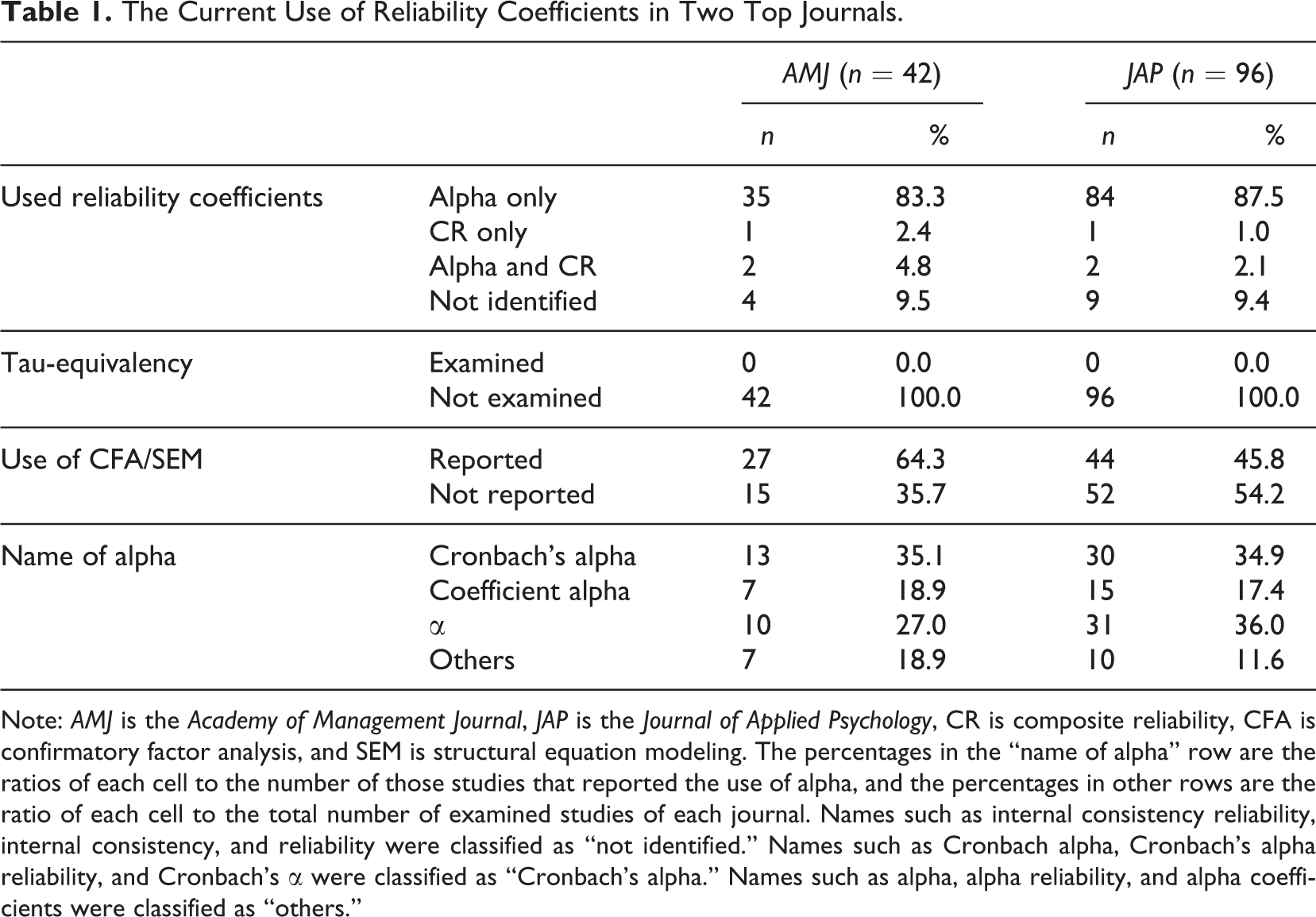
Note: AMJ is the Academy of Management Journal, JAP is the Journal of Applied Psychology, CR is composite reliability, CFA is confirmatory factor analysis, and SEM is structural equation modeling. The percentages in the “name of alpha” row are the ratios of each cell to the number of those studies that reported the use of alpha, and the percentages in other rows are the ratio of each cell to the total number of examined studies of each journal. Names such as internal consistency reliability, internal consistency, and reliability were classified as “not identified.” Names such as Cronbach alpha, Cronbach’s alpha reliability, and Cronbach’s α were classified as “Cronbach’s alpha.” Names such as alpha, alpha reliability, and alpha coefficients were classified as “others.”
Alpha’s overuse was more serious than anticipated. First, the use of SEM had little effect on the choice of reliability coefficients. Most studies that employed SEM still used alpha instead of SEM-based reliability coefficients such as composite reliability. Second, 1 in 10 studies unexpectedly did not specify the name of the utilized reliability coefficients. A plausible explanation for why researchers report reliability estimates namelessly is that they take the use of alpha for granted and thus feel little need to report a commonplace thing.
Alpha’s incorrect use was also more severe than expected. Not a single study examined tau-equivalency. That is, organizational researchers are automatically using alpha without considering whether its assumptions are satisfied. Such unconditional choice probably stems from one or some combination of the following misconceptions: Alpha is a versatile reliability coefficient that is applicable to any type of data Alpha is robust to any violation of its assumptions (i.e., even a serious violation of the assumptions has an insignificant effect on the value of the reliability estimate) A high value of alpha itself verifies that its assumptions are satisfied Identifying whether alpha’s assumptions are satisfied is difficult Alternative methods that can be used when its assumptions are violated are difficult to use
This study claims that each of the above statements is incorrect by providing formula derivations (i.e., Misconception 1), counterexamples (i.e., Misconceptions 2 and 3), illustrative examples, and an easy-to-use solution (i.e., Misconceptions 4 and 5). For example, by showing various computation examples, this study demonstrates that alpha can produce estimation errors as large as .14 when it is misapplied to data that violate one of its assumptions. In addition to disproving such misconceptions, understanding what caused them is necessary for finding a fundamental solution.
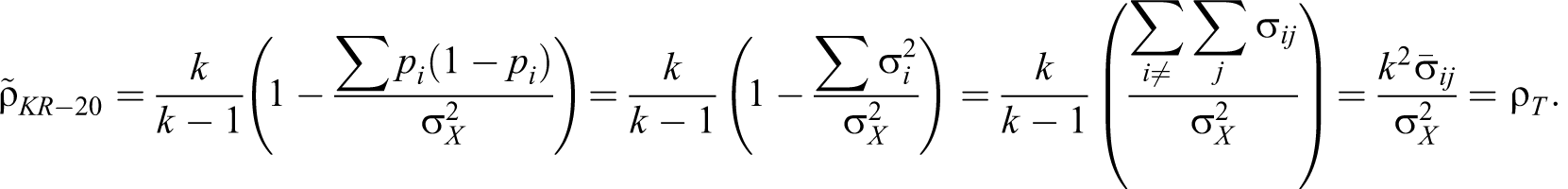
A brief review of alpha’s history is useful for identifying the underlying source of its misuse. Its popularity did not originate from its technical superiority. It became a de facto standard even at the existence of a mathematically superior predecessor (λ 2: Guttman, 1945) for several reasons that seemed important at the time of Cronbach (1951) but that are trivial from a modern view (Cho & Kim, 2015). First, alpha’s computation was simpler. Second, Cronbach (1951) positioned alpha as a reliability coefficient, whereas Guttman (1945) described λi as lower-bound estimators of reliability, which was mathematically correct but represented an unpopular description. Third, Cronbach’s (1951) proof that alpha equals the average of the reliability values (λ 4: Guttman, 1945) that are calculated for all possible split-halves positioned it as a general reliability coefficient. Although it seems intuitively attractive, the average is not as meaningful as the maximum (Osburn, 2000) or the minimum (Revelle, 1979) of the λ 4 values that are obtained from all possible split-halves (for a modern interpretation, see Hunt & Bentler, 2015). A positive feedback loop and past popularity bred today’s situation. Once the habit of unconditionally using alpha was formed, it prospered despite the development of more sophisticated methods.
Alpha’s habitual use is a matter not of mathematics but of marketing. Alpha ranked consistently low in previous comparison studies that examined the accuracy of reliability coefficients (Kamata, Turhan, & Darandari, 2003; Osburn, 2000; Revelle & Zinbarg, 2009; Tang & Cui, 2012; van der Ark, van der Palm, & Sijtsma, 2011). What differentiates alpha from other reliability coefficients is that the awareness of the name alpha outdistances that of any other reliability coefficients. In other words, its name is the main cause of its immense use. Analyzing the reason for the phenomenal citation record of Cronbach (1951), Cronbach (1978) echoed this argument by stating that “I am sure the paper is cited mostly because I put a brand name on a common-place coefficient” (p. 263).
His comments capture the essence; alpha is a brand name. The reason a researcher automatically chooses alpha without understanding its formula is analogous to the reason why a laundry detergent consumer habitually selects a familiar brand not knowing its chemical composition. Even if a comparison study were to reveal that the most popular brand underperforms its competitors, the top-of-mind brand (e.g., Gillette) would not lose significant market share. This phenomenon is what is occurring with alpha. Its use frequency remains unchanged despite the unfavorable results of several performance tests. However, if the brand name becomes null and void for some reason, its sales volume will rapidly decrease. Previous studies that placed sole reliance on a mathematical approach failed to change the 65-year-old habit. A deep-rooted problem requires a more comprehensive solution that includes a radical cure. Rebranding alpha is an efficient way to reposition it into the place where it belongs.
A Systematic Approach to Reliability Coefficients
Measurement Models
Before proceeding with the discussion, let us explain the measurement models used in this study starting from unidimensional models. Figure 1 provides a description of SEM styles regarding unidimensional parallel, tau-equivalent and congeneric measurement models. The term unidimensional will be omitted when little possibility of confusion exists. The modifiers strictly and essentially indicate whether item means are constrained to be equal. For example, an essentially tau-equivalent model includes a constant, whereas a strictly tau-equivalent model does not. Although the addition of a constant has an effect on the mean, it does not affect the variances, covariances or the value of reliability. This study focuses on essentially parallel/tau-equivalent/congeneric models and omits the term essentially for simplicity. Manifest variables (X 1, X 2, …) have a common latent variable (F) and errors (e 1, e 2, …). Errors are assumed to be purely random and independent of each other. To determine the scale, the variance of the latent variable is set to a nonzero number (typically 1.0). The congeneric model does not have additional constraints. The tau-equivalent model is the same as the congeneric model, only with the constraint that all the factor loadings are equal. The parallel model is the tau-equivalent model with the constraint that the error variances are all equal.
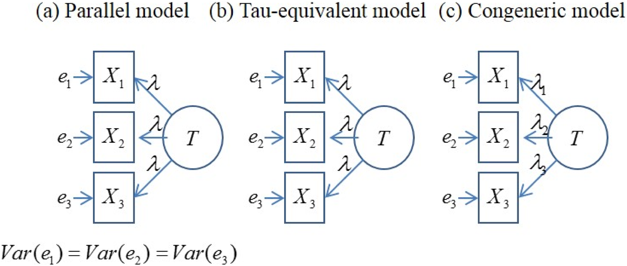
The parallel, tau-equivalent, and congeneric measurement models.
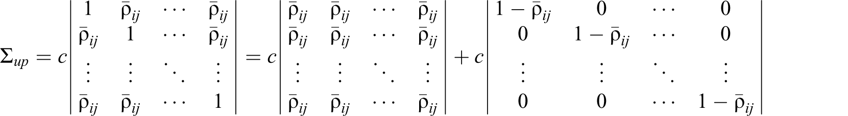
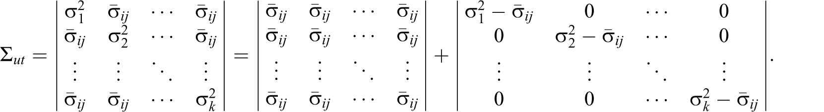
Table 2 presents interitem covariance matrices of data that perfectly satisfy the conditions of being parallel, tau-equivalent and congeneric. Covariances (i.e., off-diagonal elements of the covariance matrices) between observed item scores are determined only by the common latent variable, whereas variances (i.e., diagonal elements of the covariance matrices) of item scores are determined by the common latent variable and errors. Parallel data have equal interitem covariances and equal item variances. Tau-equivalent data have equal interitem covariances, but they may have different item variances. Congeneric data do not require the equality constraints about variances and covariances. Any parallel data are also tau-equivalent, and any tau-equivalent data are also congeneric.
Covariance Matrices of Data That Satisfy the Conditions of Being Parallel, Tau-equivalent, and Congeneric.
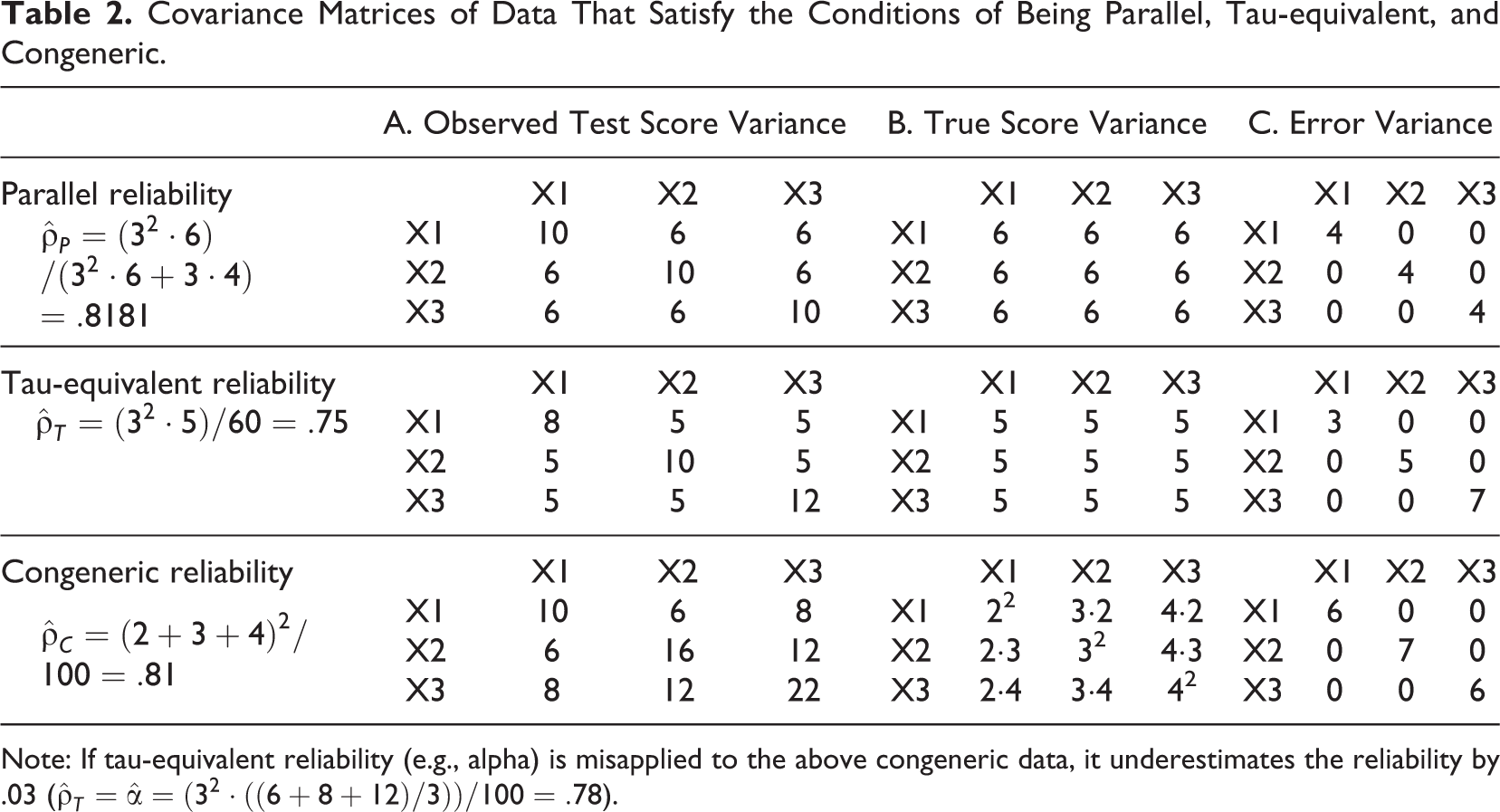
Note: If tau-equivalent reliability (e.g., alpha) is misapplied to the above congeneric data, it underestimates the reliability by .03 (
Now, let us consider multidimensional models. Three major models conceptualize multidimensionality in SEM (Figure 2): the correlated factor model, the second-order factor model, and the bifactor model. A unidimensional model consists of only a common construct (i.e., T in Figure 1) and omits subtest constructs. A correlated factor model includes only subtest constructs (i.e., Dp
in Figure 2) and neglects a common construct. The common construct of a bifactor model is called a general factor (i.e., F), and its subtest constructs are called group factors (i.e., Gp
). The common construct in a second-order factor model is called a second-order factor (i.e., Q), and its subtest constructs are called first-order factors (i.e., Op
). To determine the scale, the variances of common constructs and subtest constructs are usually set to 1.0 (i.e.,
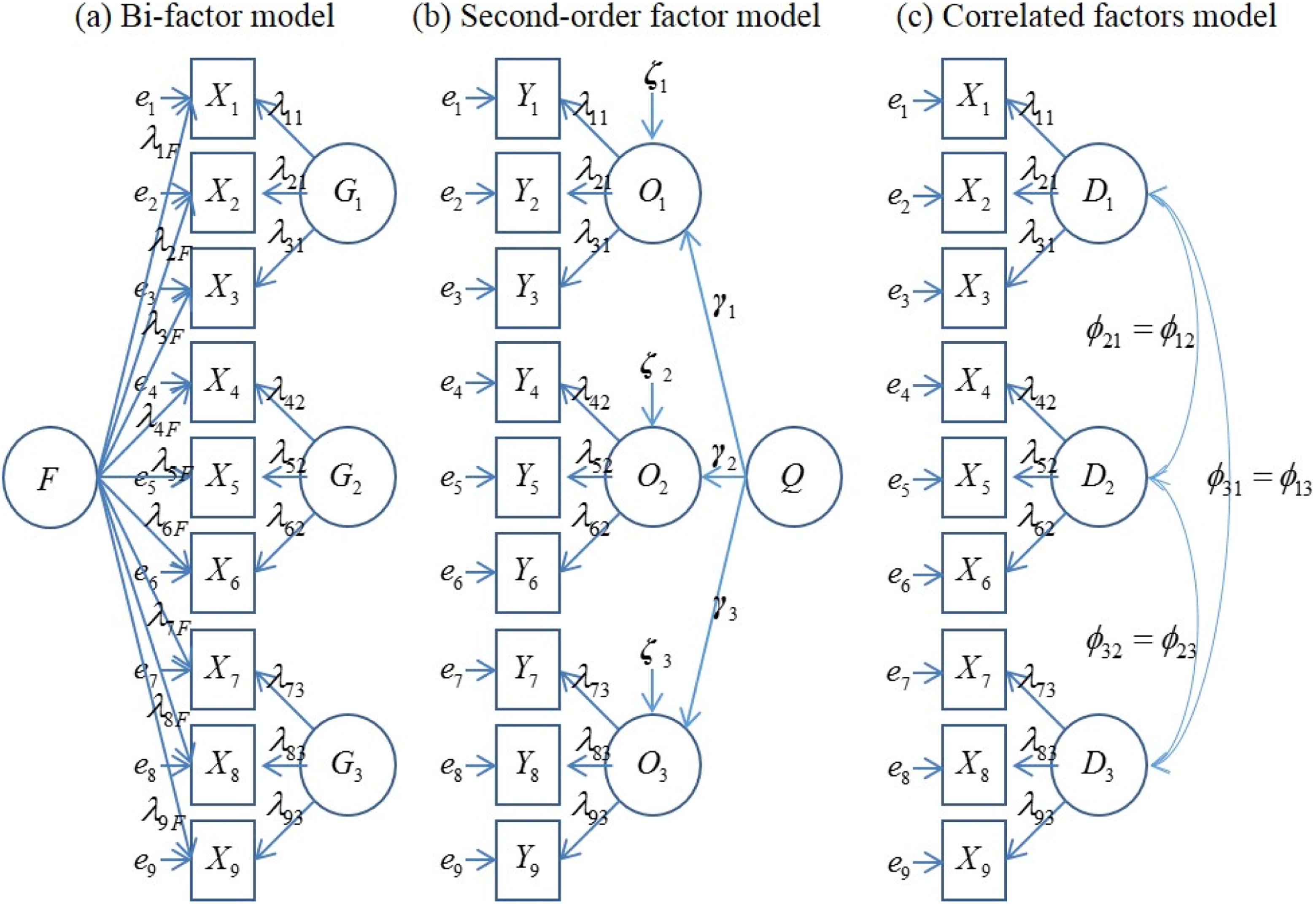
Three major multidimensional measurement models.
The bifactor model is a generalization of the second-order factor model, and the latter is nested within the former. Mathematically speaking, the latter is equivalent to the former only under the proportionality constraint (Yung, Thissen, & McLeod, 1999). Before explaining the proportionality constraint, this study notes that group factors are defined to be independent of a general factor but that first-order factors are dependent on a second-order factor. Disturbances (i.e., ζi
) are mathematically analogous to group factors because both explain the variances that are not explained by a common construct. The variance due to the disturbance is proportional to the variance due to the second-order factor between manifest variables that have the same first-order factor. For example, let us consider Y
1 and Y
2. Any effect of the second-order factor (i.e., Q) or the disturbance on Y
1 or Y
2 must be mediated by the coefficients λ
11 or λ
21.Y
1’s ratio of the variance due to the disturbance to the variance due to the second-order factor (i.e.,
This study offers a direct formula that computes the omega coefficient of a second-order factor model without a transformation. McDonald derived omega from a bifactor model. Applying its formula to a second-order factor model requires a Schmid–Leiman transformation (Schmid & Leiman, 1957) of the parameter estimates (Brunner, Nagy, & Wilhelm, 2012; Yung et al., 1999), which is unfamiliar to typical organizational researchers. A direct formula provides an easier computation and a better understanding of its meaning.
This study introduces multidimensional parallel models and multidimensional tau-equivalent models. The conditions of being parallel and tau-equivalent have only been discussed in unidimensional models in the literature. If such restrictions were so useful in deriving meaningful reliability coefficients (e.g., alpha and standardized alpha) from unidimensional models, they must be equally advantageous to multidimensional models. The second-order factor parallel model (Figure 3) requires four restrictions: The path coefficients between the second-order factor and all first-order factors are restricted to be equal to each other (i.e., γp
= γ for all p), the first-order factor loadings of all items are restricted to be equal to each other (i.e., λi
= λ for all i), all first-order factors are restricted to have equal numbers of items (i.e., np
= n for all p), and the errors of all items are restricted to be equal to each other (i.e.,

Two suggested multidimensional measurement models.
Systematic Nomenclature
Table 3 presents the names of reliability coefficients that are currently used in the literature. The conventional names of reliability coefficients are not user friendly. First, they do not deliver meaningful information to the users. For example, names such as Spearman–Brown or Flanagan–Rulon provide only the names of those who discovered these formulas without expanding on their characteristics. Although respect for these scholars is displayed, the names do not consider the needs of users.
Names of Reliability Coefficients Currently Used in the Literature.
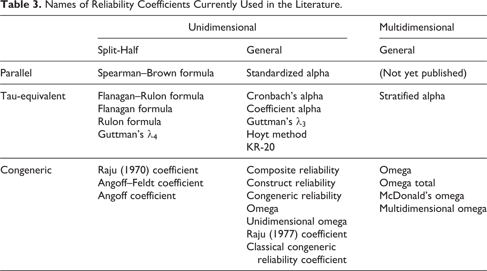
Second, the names are inconsistent. Some are called formulas (e.g., Spearman–Brown and Flanagan–Rulon), some are called coefficients (e.g., alpha), and others are called lower bounds (e.g., Guttman’s λi ). Some bear their originators’ names (e.g., Spearman–Brown), and some use a combination of the first and second developers’ names (e.g., Flanagan–Rulon). One estimator goes by the name of the fourth person to propose it (Cronbach, 1951), and others do not bear the name of any developers.
Third, they are not mutually exclusive. Formulas that are algebraically equivalent have different names, such as the Flanagan–Rulon formula and Guttman’s λ 4. Without background knowledge, users may accept these names as referring to different formulas. On the other hand, one name is used to represent multiple formulas. McDonald (1978) defined omega in a multidimensional context and later used the term regardless of the dimensionality (McDonald, 1999). Previous studies are increasingly using omega as a general name for various SEM-based reliability coefficients (Brunner et al., 2012; Cho & Kim, 2015; Dunn et al., 2013; Green & Yang, 2015; Lucke, 2005; Padilla & Divers, 2013; Revelle & Zinbarg, 2009). Whenever readers encounter the term omega, they must understand the context to know exactly which formula was used. Although methodologists may accept such mixed use as being convenient, it can confuse nonexperts. Raju coefficients also require special attention; Raju (1970, 1977) coefficients require the specification of the years of publication to avoid confusion because the researcher proposed two reliability coefficients.
Fourth, the current nomenclature is not expandable. Not all reliability coefficients have names. Table 3 indicates that a reliability estimator based on a multidimensional parallel model is a theoretically possible reliability coefficient that no one has yet formally proposed, thereby leading to its lack of a name. While generally accepted rules for naming a newly developed reliability coefficient do not exist, a naming method that was popular in the past is choosing one of the Greek letters, for example, α(Cronbach, 1951), β (Revelle, 1979), λ (Guttman, 1945), ω (Ten Berge & Zegers, 1978), θ (Armor, 1974), and ω (McDonald, 1978). This naming strategy is not sustainable because we are running short of Greek letters. Greek letters such as σ, ∊, ρ, and τ are almost exclusively used for frequently used methodological notions, and most of the remaining Greek letters (e.g., φ, ζ, γ, and ξ) are habitually used in the SEM literature. Using one of them as the name of a reliability coefficient would confuse users.
Table 4 shows the names proposed by this study. A systematic nomenclature should be informative, consistent, mutually exclusive and expandable. It should effectively and economically convey the characteristics of each method as well as their commonalities and differences. A systematic name of a reliability coefficient should also be combined with its use. For example, imagine that Fisher (1925) named the formula of two-way ANOVA (analysis of variance) after himself. We would spend a long time memorizing when to use the Fisher formula. If we rename alpha as tau-equivalent reliability, we do not need to learn the conditions under which it should be used once we know the tau-equivalent measurement model. A systematic nomenclature becomes easier once we become accustomed to it.
Names and Notations of Reliability Coefficients Suggested in This Study.
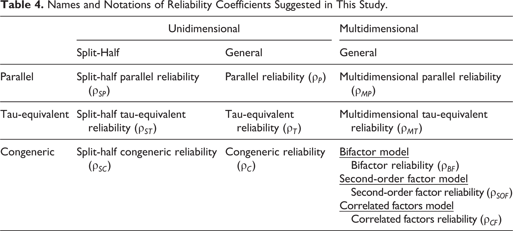
This study provides additional cautionary tales on the expressions Cronbach’s alpha and composite reliability because they are the most commonly used but misleading names. First, let us consider Cronbach’s alpha. At the time of Cronbach’s (1951) publication, this formula was already “a common-place coefficient” (Cronbach, 1978, p. 263) and usually called KR-20. Kuder and Richardson (1937) proposed several new reliability formulas but did not name them. The designation “KR-20” referred to its being the 20th formula in their article. Cronbach (1951) claimed that KR-20 was an awkward name for something that would be used frequently; thus, he proposed a new name: coefficient alpha. This name, however, had the potential to be confusing because the name alpha was regularly used in research methodology textbooks to denote other concepts such as significance level (e.g., α = .05). Thus, calling it Cronbach’s alpha would have provided the users more discernibility than simply referring to it as alpha. Such convention, however, gives a misleading impression that Cronbach first developed the formula, and Cronbach (2004) opposed the expression Cronbach’s alpha.
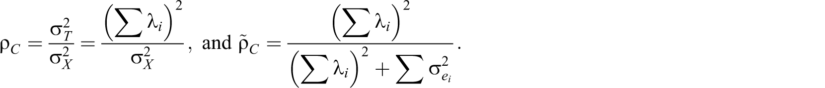
Next, let us consider composite reliability. At least seven names are used to represent a reliability estimator based on a congeneric model in the literature: composite reliability, construct reliability (e.g., Hair, Black, Babin, & Anderson, 2010), congeneric reliability (e.g., Graham, 2006; Lucke, 2005), classical congeneric reliability coefficient (Feldt & Brennan, 1989), omega (McDonald, 1999), unidimensional omega (Cho & Kim, 2015) and Raju (1977) coefficient. Among them, composite reliability is the least appropriate for the name of a specific reliability coefficient because it is shorthand for the reliability of composite scores (Cho & Kim, 2015). This name may even cause erroneous associations such as with complex or synthesized reliability. Below is my criticism in terms of history.
The originator of this formula intended to use the term congeneric, not composite. The term composite reliability first appeared in Werts, Rock, Linn, and Jöreskog (1978), in which the authors called it simply “reliability” but referred to it as “the composite reliability” once when they compared it with single-item reliability. Few pioneers of this formula called it composite reliability or any other term. It is ironic that the lack of an appropriate alternative caused the unintended name to become widely used. Jöreskog (1971) also did not suggest a special name for the reliability coefficient he developed and simply called it reliability. However, the term congeneric is what he coined to describe its measurement model. Congeneric reliability is a name that honors his contribution.
Readers should consider the parallel use of conventional and systematic names if necessary. Some conventional names, such as alpha, are too deeply embedded in our memory to remove in the short term. Even if a researcher uses only a systematic name in his or her study, the reviewers and readers are likely to be unfamiliar with it. Using both conventional and systematic names may enhance the fidelity of communication. For example, tau-equivalent reliability can be denoted as “tau-equivalent reliability (i.e., alpha).” If the systematic nomenclature becomes more common in the future, it will substitute the conventional nomenclature in the long term.
Systematic Derivation of the Formula
Although understanding how a formula was derived is the best way to understand its essence, the literature on reliability often overlooks the derivations of formulas. Four problems are associated with this practice. First, few articles comprehensively and systematically address the derivation of formulas regarding various reliability coefficients. Second, due to the lack of related research, the various original studies that discovered these formulas are being used as the sole source of derivations. Third, the derivational methods used in the original studies were not able to utilize later, more efficient methodologies, which means that the original studies use more complex methods even though simpler derivational methods have since been developed. Fourth, most reliability coefficients were derived using different sets of logic, leading to a lack of consistency in derivational methods. For example, to derive formulas that are algebraically equivalent, Hoyt (1941) used the ANOVA approach, whereas Cronbach (1951) calculated the average of the split-half reliability coefficient obtained from all possible split halves.
The current study proves that various reliability coefficients can be derived from measurement models nested within the bifactor model. The goal of the current study is to propose a derivational method for formulas that clearly reveal the basic assumptions of each reliability coefficient and the difference between each reliability coefficient. The derivations based on the unidimensional model are displayed here, and the derivations based on multidimensional models will appear in Appendix B.
The definition of reliability
Let us define test score reliability in the unidimensional model or classical true score model (Lord & Novick, 1968). Consider a test that is composed of k dichotomously or polytomously scored items. This study defines the test score X as the sum of k observed scores Xi
:
The unidimensional parallel model
The unidimensional parallel model restricts the factor loading and error variance of each item to be equal (i.e., λi
= λ and
Special case (k = 2)
Let ρ12 denote the ratio of λ2 to c. ρ 12 equals the product-moment correlation between the first and second items (or split half). The interitem covariance matrix is as follows:

The sums of the second, third, and fourth matrices are

General case
Let
The sum of the second k × k matrix (i.e.,

The unidimensional tau-equivalent model
The unidimensional tau-equivalent model (Novick & Lewis, 1967) restricts the factor loadings of each item to be equal (i.e., λi
= λ for all i). The observed score of item i is expressed as
Special case (k = 2)
Let


Flanagan (1937), Guttman (λ 4, 1945), Rulon (1939), and Mosier (1941) proposed formulas that are algebraically equivalent to ρST :


General case
Let
Cronbach (

The unidimensional congeneric model
The unidimensional congeneric model (Jöreskog, 1971) is an unrestricted base model. The observed score of item i is expressed as
Special case (k = 2)
The interitem covariance matrix and split-half congeneric reliability (ρSC ) are as follows:


This coefficient cannot be estimated without further constraints because the model is under-identified. Specifically, there are more unknowns (i.e., λ
1, λ
2,
General case
The interitem covariance matrix, the derived formula of congeneric reliability (ρC
), and the conventional version (
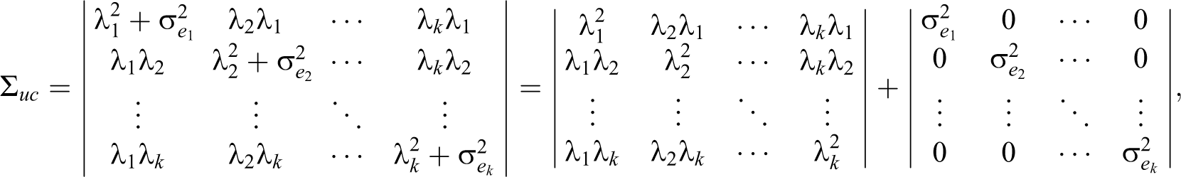
Systematic Expression of Formula
A formula may have multiple algebraically equivalent versions. For example, the definition of reliability can be expressed in several ways, including
Table 5 presents a summary of conventional formula expressions. Excluding the relationship between split-half parallel reliability (i.e., the Spearman–Brown formula) and parallel reliability (i.e., standardized alpha), no commonalities or regularities between the formulas occur. Some formulas are a subtraction of a certain value from 1, and others are not. One formula has
Conventional Formula Expressions of Reliability Coefficients.
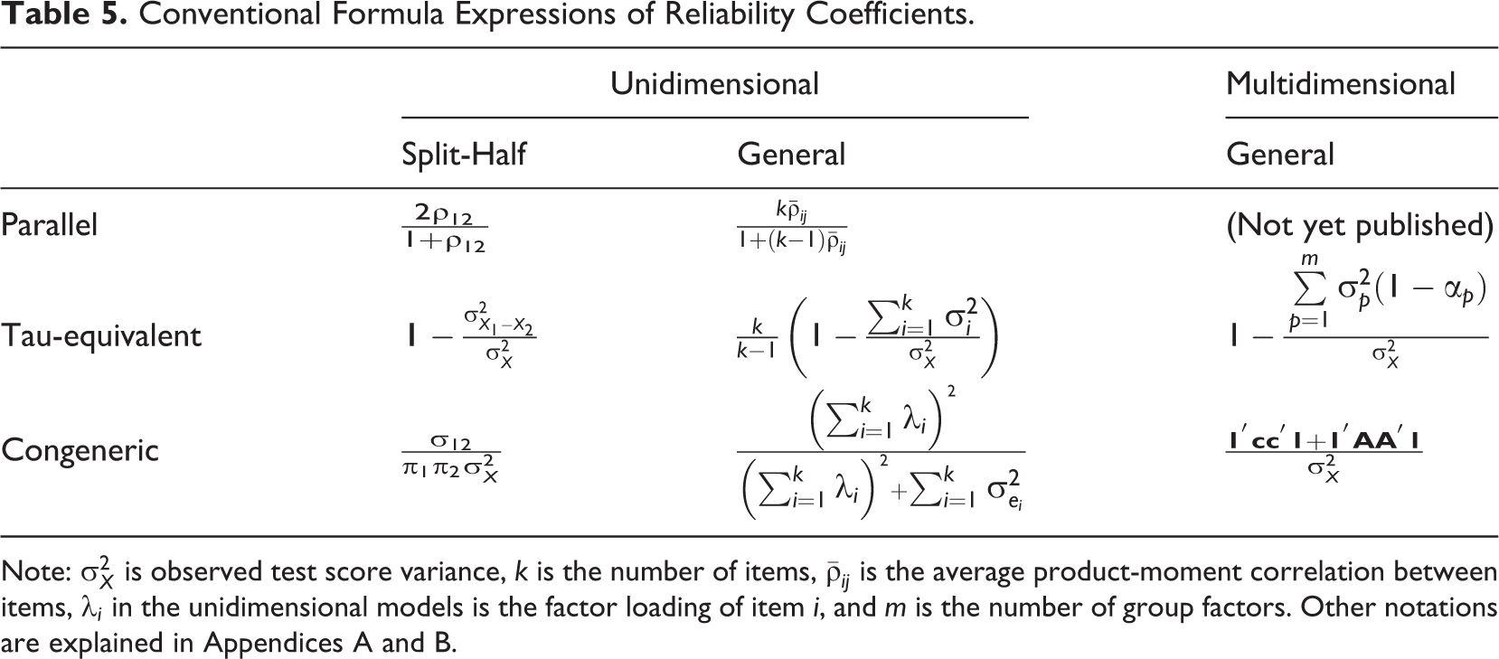
Note:
The current principle applied when expressing the formula of a reliability coefficient is that the formula expression used by the author of the original article is used. This convention is author friendly but not reader friendly. The formula expression chosen by the author and the expression easily understood by readers is different for three reasons. First, each formula is derived using different methods with various interpretations. The derivational method and the interpretation of the formulas also influenced their expression.
Second, authors are rewarded for the distinctiveness of their work, not consistency. Academia prefers studies that are different from previous studies; those that present results that are similar to existing findings are not highly regarded. Researchers may attempt to express different versions of formulas and propose different methods of interpretation.
Third, authors have preferred formula expressions that are computationally simple. Many reliability formulas were published in an era during which they could be calculated only by hand instead of with computers. Because of social inertia, computationally simpler formulas have been chosen even after computer-based computational processes became common. Thus, the most famous versions of formulas are typically those that require the fewest calculations (Falk & Savalei, 2011).
The three problems mentioned above suggest a direction for our proposed systematic formula expression. First, the system should include a consistent set of principles. Second, this study’s goal is to connect apparently disparate formulas to a degree in which users can easily recognize the common features of the formulas. Third, its goal is not to provide ease of calculation; rather, it wants to provide ease of understanding. In the current environment in which all calculations are dependent on computers, ease of calculation cannot be an important consideration for users.
Table 6 summarizes the formula expressions that the current study proposes. This study applies a consistent set of principles. More specifically, between matrix expressions and nonmatrix expressions, this study uses nonmatrix expressions. The denominator is made consistent to be
Systematic Formula Expressions of Reliability Coefficients.
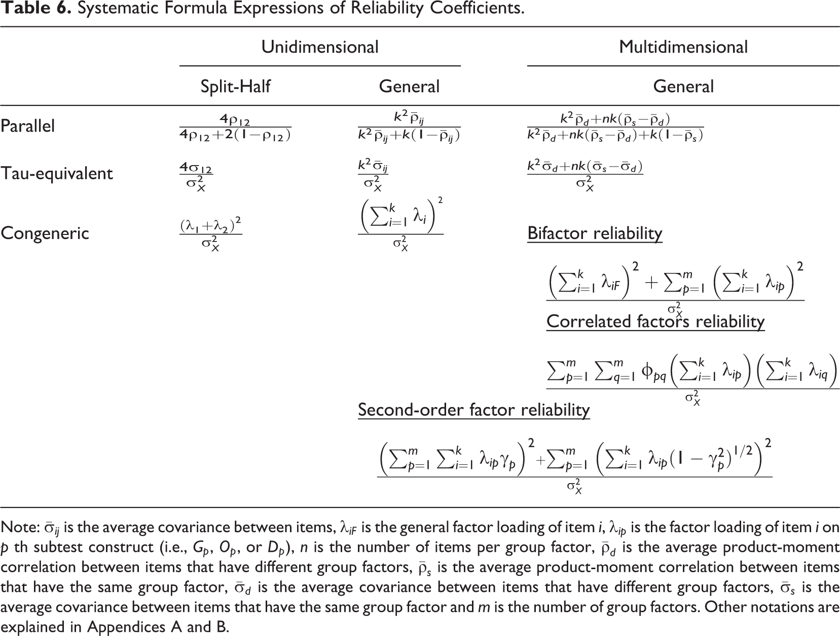
Note:
The systematic formula expressions provide us with an intuitive understanding about the condition under which reliability coefficients have a value of less than zero. The definition of reliability
This study derives two hierarchical omega coefficients from multidimensional parallel and multidimensional tau-equivalent models. McDonald (1985, 1999) proposed two definitions of reliability that are applicable to multidimensional models, and Zinbarg, Revelle, Yovel, and Li (2005) more explicitly expressed McDonald’s proposal, recommending it be categorized into ω, which were relabeled as ωt
in Revelle and Zinbarg (2009), and ωH
(or ωh
). ωH
is called hierarchical omega or omega hierarchical. The formula of the McDonald–Zinbarg hierarchical omega includes only the variance due to a general factor in the numerator (i.e.,
Four Coefficients of Hierarchical Omega.
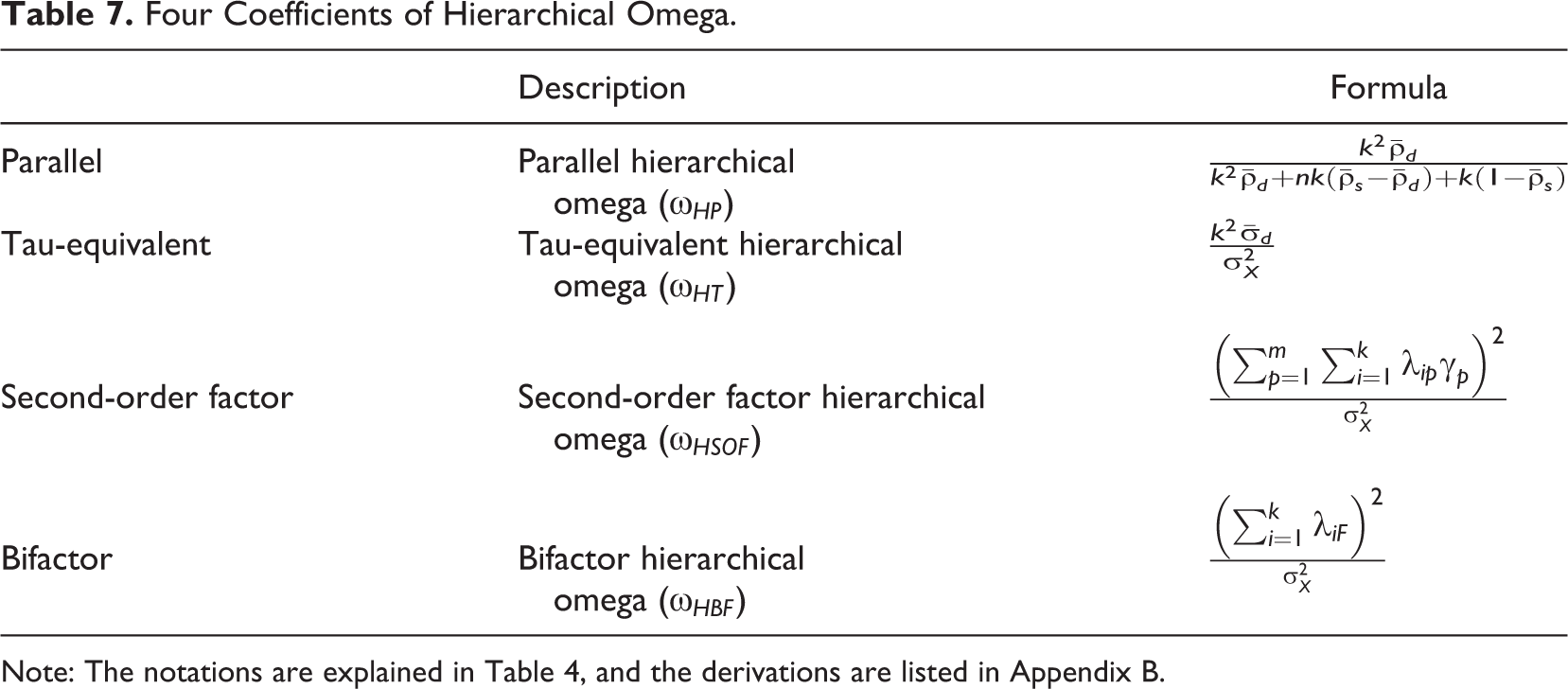
Note: The notations are explained in Table 4, and the derivations are listed in Appendix B.
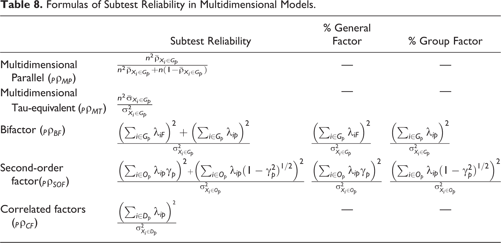
This study classifies the reliability of multidimensional models into two hierarchical levels: the reliability of a measurement model and the reliability of subtest constructs. Offering both test reliability and subtest reliability estimates may provide more complete information about the measurement. Table 8 shows the formulas of subtest reliability. Formulas of subtest reliability coefficients of multidimensional parallel, multidimensional tau-equivalent and correlated factors models are a minor modification of those of parallel reliability, tau-equivalent reliability, and congeneric reliability. Subtest reliability coefficients of bifactor and second-order factor models do not have analogous unidimensional reliability coefficients. Brunner et al. (2012) extended the concept of hierarchical omega to the subtest reliability level; however, they used the term to denote the ratio of the variances due to group factors to test score variances (i.e., % group factor in Table 8), which is different from the way Zinbarg et al. (2005) defined hierarchical omega at the test reliability level (i.e., % general factor). Because using the term hierarchical omega at the level of subtest reliability can be confusing, this study employed generic terms.
Formulas of Subtest Reliability in Multidimensional Models.
Systematic Use
Although tau-equivalent reliability (i.e., alpha) is the most popular reliability coefficient among organizational researchers, experts treat it quite differently. Previous studies are practically unanimous in declaring that there must be an alternative to the current practice of indiscriminately using this coefficient, although little consensus exists about exactly which alternative technique should replace alpha (Bentler, 2009; Green & Yang, 2009b; Hunt & Bentler, 2015; Osburn, 2000; Revelle & Zinbarg, 2009; Schmidt, Le, & Ilies, 2003; Sijtsma, 2009b; van der Ark et al., 2011). The current study does not propose a specific reliability estimator as an alternative; rather, it delineates a system composed of multiple methods.
This study does not agree with the unconditional use and denial of tau-equivalent reliability. Criticizing alpha’s unconditional use is different from advocating that another alternative should take its seat and be universally used instead. To prevent the blind use of tau-equivalent reliability, previous studies have criticized it using rather strong language. For example, Peters (2014) claimed that we should abandon alpha because it is “a fatally flawed estimate of its reliability” (p. 56). This study encourages the use of tau-equivalent reliability if the data meet the condition of being tau-equivalent. What this study disapproves of is the concept of a single best reliability coefficient that is appropriate for all types of data sets, which implicitly assumes that the objective function is one dimensional.
Any reliability coefficient in a system is not superior or inferior to another because they simply assume different measurement models. The evaluation criteria of a scientific model are at least two dimensional; a good model should explain the maximum amount of data using the fewest elements. SEM measurement models provide a trade-off between goodness of fit (i.e., chi-square) and parsimony (i.e., degree of freedom), and less parsimonious models should have significantly better goodness of fit. Unidimensional models are nested within multidimensional models, and tau-equivalent models are nested within congeneric models. When comparing two competing SEM models where one is nested within another, we typically use the chi-square difference to test significance.
Recommendations for use
Figure 4 shows a guideline for choosing a reliability coefficient. The chi-square difference test represents major statistical criteria at all steps. How to identify the dimensionality (i.e., STEP 1) of data is an important but controversial issue. Numerous methods have been proposed to test unidimensionality (Hattie, 1985). Sometimes, exploratory factor analysis or CFA can be used to examine the dimensionality of data. This study will introduce a gadget that enables users to perform CFA without SEM software.

A guideline for choosing a reliability coefficient.
Organizational researchers should combine theoretical considerations with statistical criteria when deciding which measurement model to use. A researcher’s judgment is especially important when choosing between multidimensional models (i.e., STEP 3). A bifactor model or a second-order model have a hierarchy that consists of a common construct and subtest constructs. A correlated factors model is composed of only subtest constructs. A key question is whether the researcher has a theoretical interest in a common construct and whether it has theoretical underpinnings (Brunner et al., 2012). The answer is affirmative in many cases because a common construct is what scale developers originally intended to measure and what typical researchers are most interested in (Cho & Kim, 2015; Reise, 2012). The use of correlated factor reliability is questionable because the use of a total test score of a correlated factors model is not recommended (McDonald, 1999). Brunner et al. (2012) advocated the use of only subtest reliability coefficients when a correlated factors model is selected. Reporting correlated factor reliability may have the merit of providing additional information about the measurement; however, complete reliance on it is not recommended.
Examples and a Calculator
Illustrative Examples
Understanding a formula promotes its frequent use. Organizational researchers rarely use multidimensional reliability coefficients, even though they usually study multifaceted phenomena and analyze multidimensional data. Such lack of use probably originates from their limited awareness and understanding of multidimensional reliability coefficients. The terms awareness and understanding denote different meanings here. For example, thus far, this study is likely to make readers aware of the names and formulas of multidimensional reliability coefficients but is unlikely to make the readers understand their meaning. A good way to understand a complex formula is to apply it to a simple numerical example. This study presents a unidimensional example and five multidimensional examples to make the formulas more comprehensible to readers.
Let us start from a comparison of tau-equivalent reliability and congeneric reliability. Table 9 omits the upper triangle of the covariance matrices, as done by typical SEM software packages. Readers should be careful to use the sum of the fitted or implied covariance matrix (i.e.,
A Computation of Tau-equivalent Reliability and Congeneric Reliability.
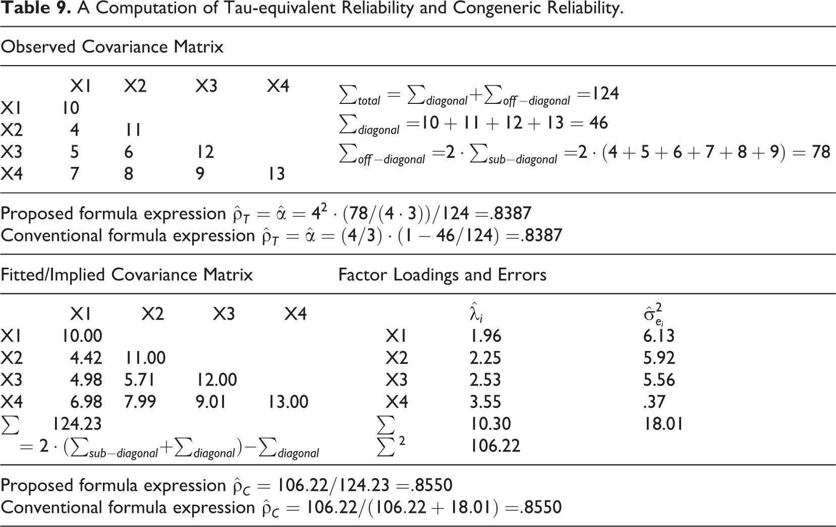
Table 10 presents a decomposition of the covariance matrix of multidimensional parallel data. Readers may find the meaning of multidimensional parallel reliability difficult to understand because it is new to them and has a complex form. The denominator of the formula of multidimensional parallel reliability, that is,
A Computation Example of Multidimensional Parallel Reliability.
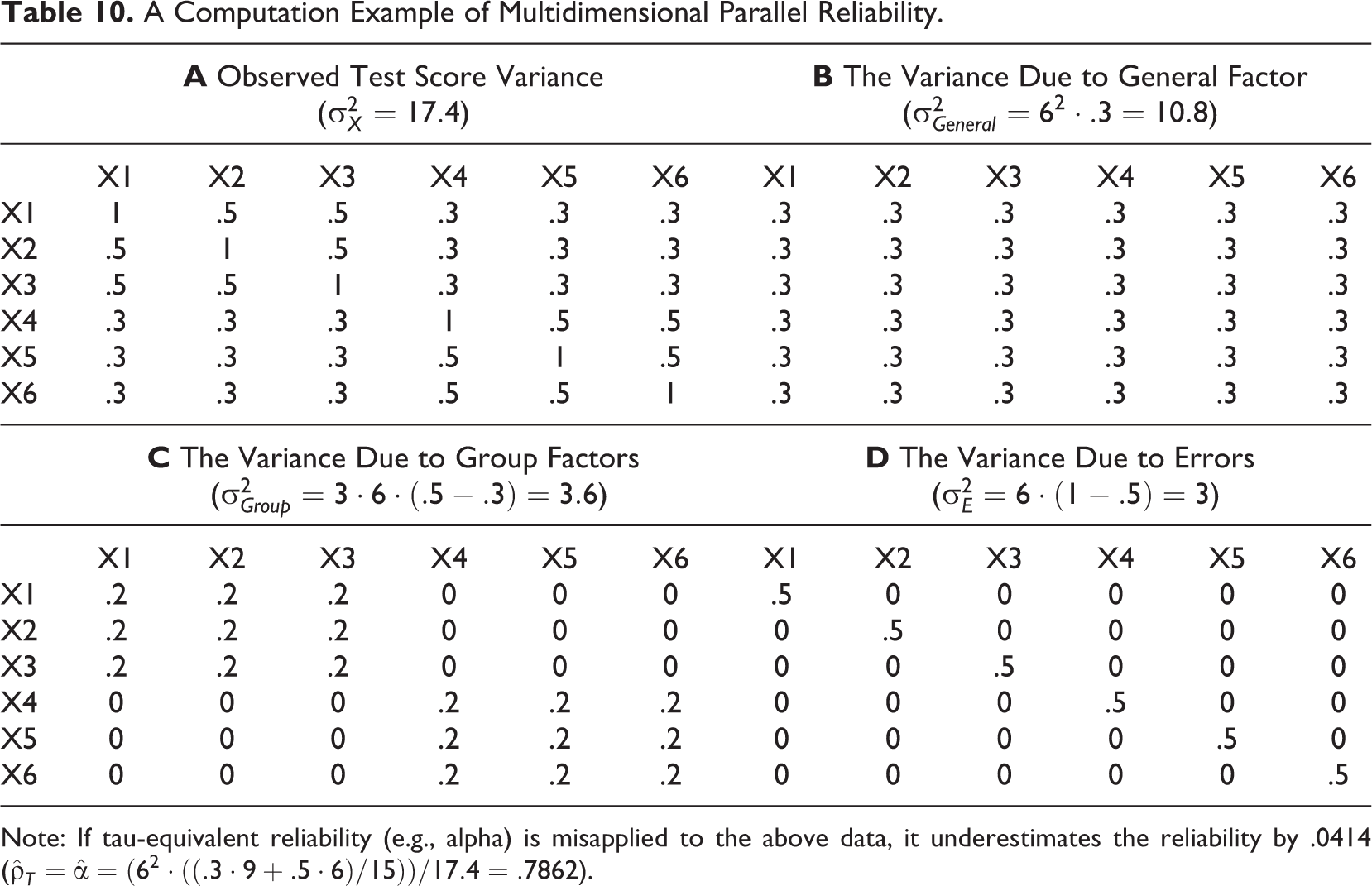
Note: If tau-equivalent reliability (e.g., alpha) is misapplied to the above data, it underestimates the reliability by .0414 (
Matrices
A Computation Example of Multidimensional Tau-equivalent Reliability.
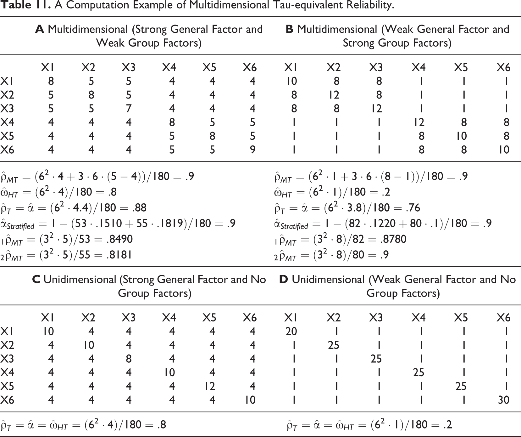
Let us further discuss the relationships between reliability, hierarchical omega and unidimensionality based on Table 11. First, unidimensionality should be identified before reliability is calculated. Many users perform the reverse; they calculate reliability to identify unidimensionality, misconceiving that a high value of a unidimensional reliability coefficient indicates unidimensionality (Cortina, 1993; Green, Lissitz, & Mulaik, 1977; Hattie, 1985; Schmitt, 1996). Table 11 disproves this misconception; the tau-equivalent reliability estimates of Matrices
Second, the concept of hierarchical omega and unidimensionality should be distinguished. A glance at Table 11 may give readers a misleading impression that the level of hierarchical omega is related with the degree of unidimensionality or homogeneity. Although hierarchical omega is a matter of degree, dimensionality is a yes-or-no issue (Zinbarg et al., 2006); all data are either unidimensional or multidimensional. Unidimensionality should be distinguished from the degree to which total test scores reflect a common construct (Reise, 2012). For example, Matrix
Third, hierarchical omega is not a substitute of reliability; it is a complement of reliability. Although hierarchical omega originated from another definition of reliability that is derived from multidimensional models, its characteristics are different from other reliability coefficients. For example, matrices
Table 12 shows a computation of bifactor reliability. The parameter estimates are
A Computation Example of Bifactor Reliability.
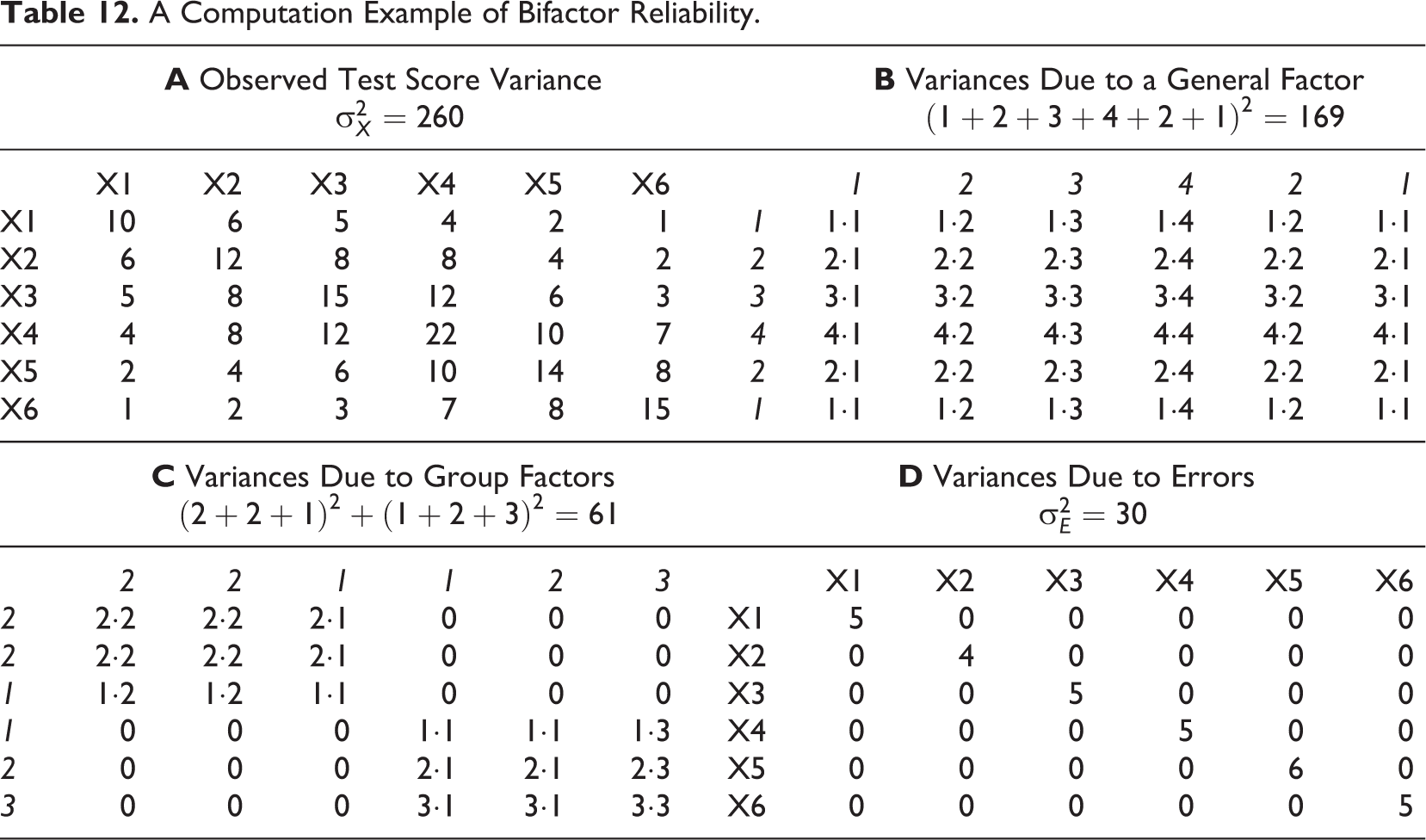
Table 13 shows a computation of second-order factor reliability. The parameter estimates are
A Computation Example of Second-order Factor Reliability.

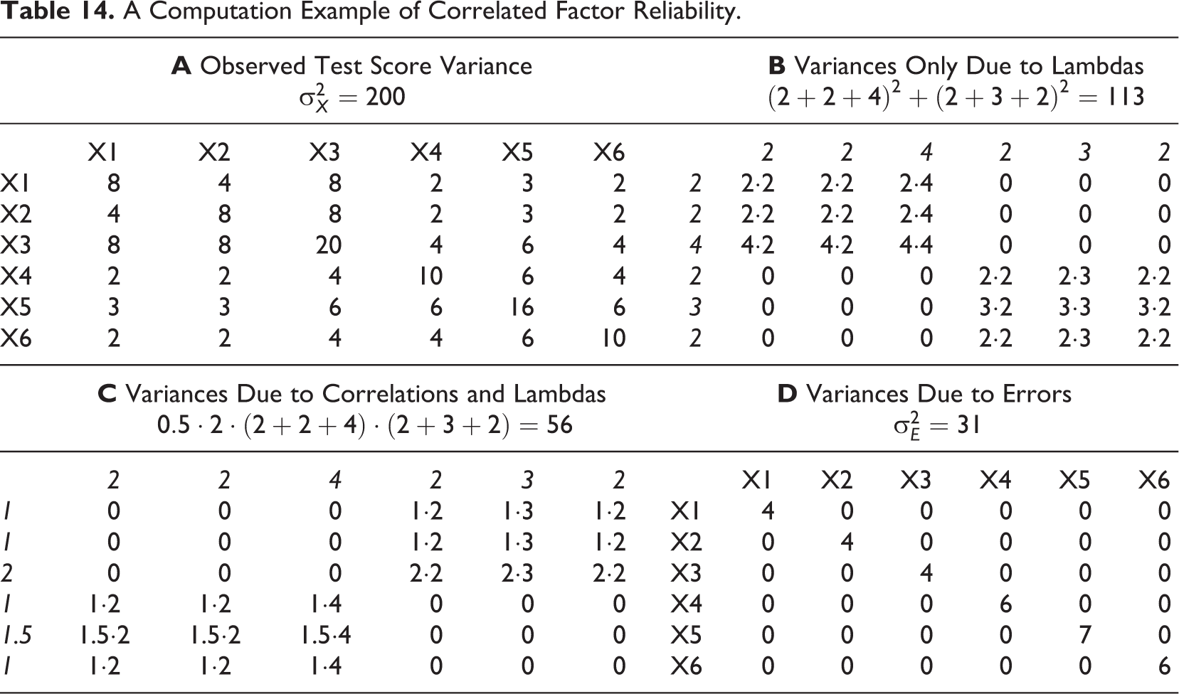
Table 14 shows a computation of the correlated factor reliability. The parameter estimates are
A Computation Example of Correlated Factor Reliability.
RelCalc: A Calculator That Computes Reliability Coefficients
A key to ending the blind use of tau-equivalent reliability (i.e., alpha) is improving the user convenience of its alternatives. Thus far, this study has provided various solutions to resolve the common misuse of reliability coefficients. Now, it offers a quick fix to the last but not least problem. Whereas popular statistical software packages such as SPSS and SAS offer an automatic calculation of tau-equivalent reliability, commonly used SEM software packages, except EQS (Bentler, 2006), do not produce SEM-based reliability estimates. Users of such programs should personally calculate the value of a reliability coefficient based on its formula. Such computations are inconvenient and susceptible to mistakes. This is a possible reason why organizational researchers who use SEM rely on tau-equivalent reliability instead of SEM-based reliability coefficients. If they could compute congeneric reliability by simply clicking a mouse, they are likely to use it substantially more frequently. I developed a calculator to overcome this obstacle. The history of reliability coefficients provides a lesson that publishing something namelessly is likely to produce an uninformative or confusing name. I call this calculator RelCalc. It is free to use and distribute. 2
RelCalc is a Microsoft Excel spreadsheet consisting of two modules. The first module is designed to help its users choose the right unidimensional reliability coefficient that fits their data. Graham (2006) gave an excellent lecture on choosing between tau-equivalent reliability and congeneric reliability. Following his advice requires readers to fully understand the statistical procedures used to examine the tau-equivalency assumption. As the results of the first section show, this teach-them-how-to-fish approach has seen little effect on how typical organizational researchers use reliability coefficients. This study adopts a give-them-a-fish approach and introduces a program that automates the required statistical procedure.
The first module examines whether the data meet the condition of being parallel or tau-equivalent and calculates three unidimensional reliability coefficients based on the user’s input of a covariance matrix. This idea originated from Miles’s (2005) suggestion that the maximum likelihood estimation, the most commonly used estimation method in SEM, is an optimization technique that finds a solution to minimize the discrepancy function, and for this, Microsoft Excel offers an optimization tool.
The second module of RelCalc can compute all multidimensional reliability coefficients that were included in this study (i.e., Tables 6, 7, and 8). Unlike the first module, the second module does not estimate the parameters of measurement models; users should copy and paste the parameter estimates that are obtained from an SEM software.
Conclusion
Reliability coefficients should be understood as building blocks of a single system rather than as a collection of completely unrelated methods. Although various formulas have been proposed to estimate the reliability of unidimensional data, they all start from a single formula: the ratio of true score variance to test score variance. Because the variance of a sum is equal to the sum of all elements in the covariance matrix of the components, we are actually discussing the covariance matrix. This study demonstrated the decomposition of covariance matrix for estimating reliability based on SEM models. We do not require a dozen names for reliability coefficients that are seemingly unrelated or a dozen formula expressions that are seemingly unrelated; we need only a single principle that connects all these reliability coefficients.
Footnotes
Appendix A
Appendix B
Acknowledgments
I am deeply grateful to Adam Meade, associate editor, and three anonymous reviewers for their invaluable guidance and constructive comments. I also appreciate helpful support from Kyung Su Liu, Seonghoon Kim, Yanyun Yang, Richard Zinbarg, Peter M. Bentler, and Jiheon Kim. All errors are my sole responsibility.
Declaration of Conflicting Interests
The author declared no potential conflicts of interest with respect to the research, authorship, and/or publication of this article.
Funding
The author(s) disclosed receipt of the following financial support for the research, authorship and/or publication of this article: The present research has been conducted by the Research Grant of Kwangwoon University in 2015.